


ABSTRACT
High-redshift quasars are important tracers of structure and evolution in the early universe. However, they are very rare and difficult to find when using color selection because of contamination from late-type dwarfs. High-redshift quasar surveys based on only optical colors suffer from incompleteness and low identification efficiency, especially at  . We have developed a new method to select
  quasars with both high efficiency and completeness by combining optical and mid-IR Wide-field Infrared Survey Explorer (WISE) photometric data, and are conducting a luminous
  quasar survey in the whole Sloan Digital Sky Survey (SDSS) footprint. We have spectroscopically observed 99 out of 110 candidates with z-band magnitudes brighter than 19.5, and 64 (64.6%) of them are quasars with redshifts of
  and absolute magnitudes of
  . In addition, we also observed 14 fainter candidates selected with the same criteria and identified 8 (57.1%) of them as quasars with
  . Among 72 newly identified quasars, 12 of them are at
  , which leads to an increase of ∼36% of the number of known quasars at this redshift range. More importantly, our identifications doubled the number of quasars with
  at
at  , which will set strong constraints on the bright end of the quasar luminosity function. We also expand our method to select quasars at z ≳ 5.7. In this paper we report the discovery of four new luminous z ≳ 5.7 quasars based on SDSS–WISE selection.
Export citation and abstract BibTeX RIS
1. INTRODUCTION
As the most luminous non-transient objects that can be observed in the early universe, high-redshift quasars are important tracers to study early structure formation and the history of cosmic reionization (e.g., Fan et al. 2006a). In addition, understanding the evolution of quasars from the early universe to the present epoch allows us to study the accretion history of supermassive black holes (SMBHs). However, high-redshift quasar searches are highly challenging due to their low spatial density and a high rate of contamination from cool dwarfs when using the traditional multicolor selection method.
With the increasing number of large surveys such as the 2dF Quasar Redshift Survey (2QZ; Croom et al. 2001) and the Sloan Digital Sky Survey (SDSS; York et al. 2000), the number of known quasars has been increasing rapidly. The 2QZ identified more than 23,000  quasars (Croom et al. 2004). The first two phases of the SDSS spectroscopically identified more than 100,000 quasars (Schneider et al. 2010) and the Baryonic Oscillation Spectroscopic Survey (BOSS; Dawson et al. 2013), which is the third phase of SDSS (SDSS-III; Eisenstein et al. 2011), spectroscopically identified more than 300,000 quasars (e.g., Pâris et al. 2012, 2014) selected by using the extreme deconvolution method (Bovy et al. 2011; DiPompeo et al. 2015). However, most of these quasars are selected based on optical colors only and mostly at lower redshift (
 3.5). Based on SDSS g − r/r − i and r − i/i − z colors, several hundred
  quasars and some
  quasars have been discovered (Fan et al. 1999, 2000a, 2001b; Zheng et al. 2000; Anderson et al. 2001; Schneider et al. 2001; Chiu et al. 2005). These quasar surveys have to make a very strict r − i/i − z cut and suffer from low completeness to avoid the strong contamination of late-type stars. Nonetheless, the success rate of finding
  quasars in automated spectroscopic surveys remains quite low. For example, the overall success rate of finding
  quasars in the SDSS quasar survey is less than 10%.
Cool et al. (2006) discovered three  quasars in the AGN and Galaxy Evolution Survey (AGES; Kochanek et al. 2012) with targets selected from Spitzer Space Telescope mid-infrared photometry. The combination of optical and near-IR colors can improve the success rate and completeness of selecting high-redshift quasars. McGreer et al. (2013) identified 73
  quasars out of 92 candidates by adding near-IR J-band photometry. However, this method can be applied only to a narrow redshift range (McGreer et al. 2013).
Spectroscopic followup of SDSS i-dropout objects has identified more than 30 luminous  quasars (Fan et al. 2000b, 2001a, 2003, 2004, 2006b; Jiang et al. 2008, 2009, 2015). The Canada–France High-z Quasar Survey (CFHQS) has found 20 fainter
  quasars based on multicolor optical imaging at the Canada–France–Hawaii Telescope (CFHT; Willott et al. 2007, 2009, 2010a, 2010b). The Panoramic Survey Telescope & Rapid Response System 1 (Pan-STARRS1, PS1 Kaiser et al. 2002, 2010) high-redshift quasar survey has discovered more than ten
  quasars (Morganson et al. 2012; Bañados et al. 2014). Recently, Bañados et al. (2015) improved the efficiency for selecting z ∼ 6 quasars by matching Pan-STARRS1 and Faint Images of the Radio Sky at Twenty Centimeters (FIRST, Becker et al. 1995) and Carnall et al. (2015) obtained a cleaner z ≳ 5.7 candidate sample by matching optical photometry from the Very Large Telescope Survey Telescope ATLAS survey (Shanks et al. 2015) and Wide-field Infrared Survey Explorer (WISE) photometry. However, these methods can be used to select only
  quasars. The first
  quasar, ULAS J112001.48+064124.3 at z = 7.1, was discovered in the United Kingdom Infrared Deep Sky Survey (UKIDSS) Large Area Survey (LAS; Lawrence et al. 2007) by Mortlock et al. (2011). Recently, six more
  quasars (Venemans et al. 2013, 2015) were discovered in the Visible and Infrared Survey Telescope for Astronomy (VISTA) Kilo-Degree Infrared Galaxy survey (VIKING; Arnaboldi et al. 2007) and Pan-STARRS1 survey. To date, although more than 300,000 quasars are known, among them are about 170 quasars at
  , ∼60 quasars at
  and one quasar at
  . In addition there is an obvious gap of known quasars at
  , which is caused by their optical colors being very similar to those of late-type stars, especially M dwarfs. This redshift distribution gap of known quasars poses challenges for the studies of the high-redshift quasar luminosity function (QLF), the black hole mass function (BHMF) and the properties of the post-reionziation intergalactic medium (IGM).
NASA's WISE (Wright et al. 2010) mapped the sky at 3.4, 4.6, 12, and 22 μm (W1, W2, W3, and W4) with an angular resolution of 6.1, 6.4, 6.5, and 12.0 arcsec and 5σ photometric sensitivity better than 0.08, 0.11, 1, and 6 mJy (corresponding to 16.5, 15.5, 11.2, and 7.9 Vega magnitudes) in these four bands, respectively. The WISE All-Sky Data Release11 includes all data taken during the WISE full cryogenic mission phase from 2010 January 7 to August 6 and consists of over 563 million objects. Recently the ALLWISE12 program combined data from the WISE cryogenic and NEOWISE (Mainzer et al. 2011) post-cryogenic survey phases to form the most comprehensive view of the full mid-infrared sky. The ALLWISE photometric catalog includes over 747 million objects with enhanced photometric sensitivity and accuracy and improved astrometric precision compared to the WISE All-Sky Data Release.
In this paper we present a new robust method for selecting luminous high-redshift quasars by combining ALLWISE and SDSS photometric data and provide the results of optical spectroscopy followup observations. This paper is organized as follows. In Section 2 we summarize the ALLWISE detection rate of high-redshift quasars and the W1–W2 colors of high-redshift quasars and late-type stars. In Section 3 we describe our target selection and spectroscopic observations. In Section 4 we present our spectroscopic quasar sample and in Section 5 we discuss the pros and cons of our selection method and compare with the SDSS high-redshift quasar selection method. In Section 6 we extend our selection method to z ≳ 5.7 quasars and present the discovery of four new quasars at  and in Section 7 we give a brief summary. Throughout the paper, SDSS magnitudes are reported on the asinh system (Lupton et al. 1999), and WISE magnitudes are on the Vega system. We adopt a standard ΛCDM cosmology with Hubble constant
  , and density parameters
  and
and  .
.
2. WISE PHOTOMETRY OF PUBLISHED HIGH-REDSHIFT QUASARS
Wu et al. (2012) first studied SDSS quasars in the WISE preliminary data release13
sky coverage and found that WISE can detect more than 50% of the SDSS quasars with  and W1–W2
  and can separate late-type stars and quasars efficiently. Remarkably, this method has been used in the Large Sky Area Multi-object Fiber Spectroscopic Telescope (LAMOST) Quasar Survey and has discovered several thousand new quasars mainly at
  (Ai et al. 2016). The depth of ALLWISE has improved from the early catalogs, due to the stacking of multiple epoch photometry; the 95% completeness limits of ALLWISE W1 and W2 are at about 17.1 (44 μJy) and 15.7 (88 μJy) magnitude.14
Figure 1 shows the absolute magnitudes at  of a low redshift type I quasar template (Glikman et al. 2006) as a function of redshift at the ALLWISE W1 and W2 magnitude limits. It is clear that the ALLWISE data set has a high completeness of detecting luminous high-redshift quasars (e.g.,
  at
at  and
and  at
at  ) and is a highly valuable data set for finding luminous high-redshift quasars when combined with other optical sky surveys such as SDSS, PanSTARRS, SkyMapper, DES, VST ATLAS, DECaLS, and LSST as well as with near-IR surveys such as UKIDSS-LAS, UKIDSSS-UHS, and VISTA-VHS.

Figure 1. M1450 as a function of redshift for a type I quasar template from Glikman et al. (2006). The red solid line denotes W1 = 17.1 and the blue dashed line denotes W2 = 15.7, which are the 95% completeness limits of the ALLWISE catalog. ALLWISE is a promising data set for finding high-redshift quasars with high luminosity (e.g.,  at
at  and
and  at
at  ).
).
Download figure:
Standard image High-resolution imageWe collected 725 published quasars at  from the SDSS quasar catalogs and the literature (Table 1). We cross-matched these high-redshift quasars with the ALLWISE source catalog using a position offset within
  and found that 530 (73.1%) of them were detected in the ALLWISE W1 band, 505 (69.7%) in the W2 band, 261 (36.0%) in the W3 band, and 94 (13.0%) in the W4 band. In Figure 2 we show the redshift and z-band magnitude distribution of these quasars as well as the dependence of the ALLWISE detection rate on the redshift and magnitude. The ALLWISE data set detected ≳50% of the known quasars over almost all redshifts and
  % of the known quasars with
  . This is consistent with what we find in Figure 1. In particular, 34 of 50 (68%) published
  quasars are detected by the ALLWISE data set, which is higher than the result reported in previous studies on the WISE All-Sky detection rate (17/31, 55%) of
  quasars based on a smaller sample (Blain et al. 2013). Note that the drop in the detection rate at the brightest end is caused by the fact that one of three quasars in the brightest bin is blended by a nearby bright star in the ALLWISE image.

Figure 2. Upper panel: the black solid line denotes the redshift histogram of all published  quasars, while the red dashed line is the redshift histogram of the ALLWISE-detected
  quasars. The ratio between them (blue dashed line) is also plotted as a function of redshift. Note that the drop in the detection rate at
  is mainly affected by the statistic error because of the small number of objects in the bin. Lower panel: the black solid line denotes the SDSS z-band magnitude histogram of
  quasars with SDSS detections, while the red dashed line is the z-band magnitude histogram of the ALLWISE-detected
  quasars. The ratio between them is also plotted as a function of magnitude.
Download figure:
Standard image High-resolution imageTable 1.
Optical and WISE Photometry of 725 Published  Quasars
| Name | Redshift | Ref | r |

|
i |

|
z |

|
Opt | W1 |

|
W2 |

|
WISE |
|---|---|---|---|---|---|---|---|---|---|---|---|---|---|---|
| J000239.39+255034.80 | 5.800 | 16 | 23.09 | 0.32 | 21.51 | 0.11 | 18.96 | 0.05 | DR10 | 16.16 | 0.06 | 15.54 | 0.13 | AW |
| J000552.34–000655.80 | 5.850 | 16 | 24.97 | 0.51 | 22.98 | 0.28 | 20.41 | 0.13 | DR10 | 17.30 | 0.16 | 17.04 | 99.0 | AW |
| J000651.61–620803.70 | 4.510 | 51 | 18.29 | 99.0 | 99.0 | 99.0 | 99.0 | 99.0 | REF | 15.20 | 0.03 | 14.61 | 0.04 | AW |
| J000749.17+004119.61 | 4.780 | DR12 | 21.36 | 0.06 | 19.97 | 0.03 | 19.84 | 0.08 | DR10 | 16.85 | 0.11 | 16.41 | 0.26 | AW |
| J000825.77–062604.60 | 5.929 | 24 | 23.91 | 0.59 | 23.55 | 0.63 | 20.01 | 0.14 | DR10 | 16.81 | 0.11 | 15.68 | 0.14 | AW |
| J001115.24+144601.80 | 4.964 | DR12 | 19.48 | 0.02 | 18.17 | 0.02 | 18.03 | 0.03 | DR10 | 15.29 | 0.04 | 14.69 | 0.06 | AW |
| J001207.79+094720.23 | 4.745 | DR12 | 21.40 | 0.07 | 19.81 | 0.04 | 19.86 | 0.10 | DR10 | 16.26 | 0.07 | 15.80 | 0.17 | AW |
| J001529.86–004904.30 | 4.930 | 32 | 22.59 | 0.15 | 20.99 | 0.05 | 20.56 | 0.12 | DR10 | 99.0 | 99.0 | 99.0 | 99.0 | 99 |
| J001714.68–100055.43 | 5.011 | DR7 | 21.23 | 0.06 | 19.45 | 0.03 | 19.55 | 0.09 | DR10 | 15.94 | 0.06 | 15.17 | 0.09 | AW |
| J002208.00–150539.76 | 4.528 | 50 | 19.39 | 0.03 | 18.75 | 0.02 | 18.54 | 0.04 | DR10 | 15.54 | 0.05 | 15.11 | 0.10 | AW |
Note. Table 1 is available in its entirety in the electronic edition of the journal. The first 10 rows are shown here for guidance regarding its form and content. The names here are in the format of JHHMMSS.SS+/–DDMMSS.SS. The Ref column lists the reference for each quasar and the Opt column lists the references for the optical magnitudes. Most optical magnitudes are from the SDSS DR10 photometric catalog and are Galactic extinction corrected SDSS PSF asinh magnitudes ( mag). The optical magnitudes come from the reference paper and are in the AB system if the quasar does not have SDSS DR 10 photometry. The WISE column lists the flag from the WISE data: AW = ALLWISE catalog, AWR = ALLWISE Reject catalog, AS = ALL-SKY WISE catalog, ASR = ALL-SKY WISE Reject catalog, and 99 means no detection in any WISE catalog. This table only includes quasars that were published before 2015 July.
Only a portion of this table is shown here to demonstrate its form and content. A machine-readable version of the full table is available.
Download table as: DataTypeset image
Due to their red optical colors, late-type stars (especially M dwarfs) are the most serious contaminants in selecting  quasar candidates using optical colors (e.g., Fan et al. 1999). Wu et al. (2012) studied the color distributions of WISE-detected quasars and stars with SDSS spectroscopy and found that both normal and late-type stars can be well rejected with W1–W2
  (see Figure 6 in Wu et al. 2012). Figure 3 shows the W1–W2 color of quasars as a function of redshift. To have a clear view of the color-redshift track, we plot quasars with both W1 and W2 having a signal-to-noise ratio great than five as blue points and quasars with only W1 at the five sigma level as open black cycles in Figure 3. To get a more reasonable statistics of known quasars, we only count quasars detected by ALLWISE with both W1 and W2 at the five sigma level in the lower panel in Figure 3. Clearly most high-redshift quasars, especially
  quasars, have a red W1–W2 color. There are ∼41% of
  quasars having red W1–W2 colors with W1–W2
  , ∼68% of
  quasars with W1–W2
  , and ∼92% of
  quasars with W1–W2
  . Because WISE data have a high detection rate of luminous high-redshift quasars and can provide an effective way of separating quasars and late-type stars, we are conducting a luminous quasar survey at
  by combing SDSS and ALLWISE photometry. Note that there is a glaring gap of known quasars at
  which can be seen in both Figures 1 and 3. This is because quasar colors are very similar to those of M dwarfs and hard to distinguish in both optical and near-IR wavelengths. Benefiting from the different W1–W2 colors of quasars and M dwarfs, we expect that we can select
  quasars more effectively by combining SDSS and ALLWISE photometry than previous quasar selection methods.

Figure 3. Upper: the W1–W2 vs. redshift diagram. The purple dashed line represents W1–W2  . The red solid line represents the color-z relation predicted using the quasar template from Glikman et al. (2006). The solid squares from left to right mark the color tracks for quasars from z = 5.0 to z = 7.0 in steps of
  . The blue points represent
  quasars detected by ALLWISE with both W1 and W2 at the 5σ level. The black open cycles denote
  quasars detected by ALLWISE with only W1 at the 5σ level. Lower: the fraction of
  quasars with W1–W2
  as a function of redshift. Note that we only consider quasars detected by ALLWISE with both W1 and W2 at the 5σ level here. The purple dashed line denotes a fraction of 50%. We calculated the fraction using a redshift bin of 0.2. Note that the bins at
  and
and  are not plotted due to no available data. The drop of the fraction at z ∼ 6 is partly because of the large uncertainties of WISE photometry for faint high-redshift quasars.
Download figure:
Standard image High-resolution imageTable 2.
Observational Information of 72 Newly Identified  Quasars
| Name | Telescope | Grating | Slit | Redshift | Date | Exposure (s) |
|---|---|---|---|---|---|---|
| J000754.08–031730.82 | ANU | R3000 | 1.0 | 4.76 | 20141016 | 1800 |
| J000851.43+361613.49 | LJT | G12 | 1.8 | 5.17 | 20131127 | 2100 |
| J002526.84–014532.51 | MMT | 270 gpm | 1.0 | 5.07 | 20140110 | 600 |
| J003941.03+202554.85 | 216 | G4 | 2.3 | 4.61 | 20141117 | 3600 |
| J004508.81+374334.91 | LJT | G5 | 1.8 | 4.62 | 20141003 | 1800 |
| J005527.18+122840.67 | LJT | G3 | 1.8 | 4.70 | 20131125 | 1800 |
| J011614.30+053817.70 | Bok | R400 | 2.5 | 5.33 | 20141028 | 2100 |
| J012026.86+223058.55 | MMT | 270 gpm | 1.5 | 4.59 | 20140110 | 600 |
| J012220.29+345658.43 | LJT | G5 | 1.8 | 4.85 | 20140121 | 1800 |
| J012247.35+121624.06 | LJT | G5 | 1.8 | 4.79 | 20141024 | 2400 |
| J013127.34–032100.19 | LJT | G3 | 1.8 | 5.18 | 20131125 | 1500 |
| J013224.89–030718.45 | ANU | R3000 | 1.0 | 4.83 | 20150720 | 1200 |
| J013238.33+292602.57 | Bok | R400 | 2.5 | 4.45 | 20141030 | 2400 |
| J014741.53–030247.88 | 216 | G4 | 2.3 | 4.75 | 20141117 | 1800 |
| J015533.28+041506.74 | Bok | R400 | 2.5 | 5.37 | 20141028 | 2400 |
| J015618.99–044139.88 | MMT | 270 gpm | 1.5 | 4.94 | 20140110 | 600 |
| J020139.04+032204.73 | 216 | G4 | 2.3 | 4.57 | 20141117 | 3600 |
| J021624.16+230409.47 | Bok | R400 | 2.5 | 5.26 | 20141030 | 3000 |
| J021736.76+470826.48 | MMT | 270 gpm | 1.0 | 4.81 | 20140108 | 600 |
| J022055.59+473319.34 | 216 | G4 | 2.3 | 4.82 | 20141116 | 3600 |
| J022112.62–034252.26 | LJT | G3 | 1.8 | 5.02 | 20131125 | 2700 |
| J024601.95+035054.12 | LJT | G5 | 1.8 | 4.96 | 20140121 | 1800 |
| J024643.78+061045.74 | Bok | R400 | 2.5 | 4.57 | 20141028 | 2100 |
| J025121.33+033317.42 | LJT | G3 | 1.8 | 5.00 | 20131125 | 2400 |
| J030642.51+185315.85 | LJT | G3 | 1.8 | 5.36 | 20131125 | 1320 |
| J032407.69+042613.29 | Bok | R400 | 2.5 | 4.72 | 20141028 | 2100 |
| J045427.96–050049.38 | Bok | R400 | 2.5 | 4.93 | 20141117 | 1500 |
| J065330.25+152604.71 | MMT | 270 gpm | 1.0 | 4.90 | 20140109 | 600 |
| J073231.28+325618.33 | MMT | 270 gpm | 1.0 | 4.76 | 20150509 | 300 |
| J074749.18+115352.46 | LJT | G3 | 1.8 | 5.26 | 20131127 | 2100 |
| J075332.01+101511.68 | Bok | R400 | 2.5 | 4.89 | 20141111 | 2400 |
| J080306.19+403958.96 | Bok | R400 | 2.5 | 4.79 | 20141118 | 2400 |
| J083832.31–044017.47 | LJT | G12 | 1.8 | 4.75 | 20140225 | 1800 |
| J085942.62+443115.97 | MMT | 270 gpm | 1.0 | 4.57 | 20150314 | 200 |
| J111700.43–111930.63 | LJT | G5 | 1.8 | 4.40 | 20150221 | 1800 |
| J120829.27+394339.72 | MMT | 270 gpm | 1.0 | 4.94 | 20120527 | 300 |
| J122342.16+183955.39 | MMT | 270 gpm | 1.0 | 4.55 | 20150508 | 300 |
| J133257.45+220835.91 | MMT | 270 gpm | 1.0 | 5.11 | 20140109 | 600 |
| J143704.81+070807.71 | LJT | G5 | 1.8 | 4.93 | 20150214 | 1800 |
| J152302.90+591633.04 | 216/MMT | 270 gpm | 1.0 | 5.11 | 20150314 | 600 |
| J155657.36–172107.55 | LJT | G5 | 1.8 | 4.75 | 20150228 | 1500 |
| J160111.16–182835.08 | MMT | 270 gpm | 1.0 | 5.06 | 20150508 | 300 |
| J162045.64+520246.65 | MMT | 270 gpm | 1.5 | 4.79 | 20130418 | 900 |
| J162315.28+470559.90 | LJT | G5 | 1.8 | 5.13 | 20140405 | 2100 |
| J162838.83+063859.14 | MMT | 270 gpm | 1.0 | 4.85 | 20150313 | 500 |
| J163810.39+150058.26 | MMT | 270 gpm | 1.0 | 4.76 | 20140514 | 900 |
| J165635.46+454113.55 | LJT | G5 | 1.8 | 5.34 | 20141001 | 1800 |
| J175114.57+595941.47 | 216 | G10 | 2.3 | 4.83 | 20140507 | 3600 |
| J175244.10+503633.05 | MMT | 270 gpm | 1.5 | 5.02 | 20130418 | 900 |
| J205442.21+022952.02 | MMT | 270 gpm | 1.0 | 4.56 | 20150508 | 300 |
| J211105.62–015604.14 | LJT | G5 | 1.8 | 4.85 | 20140708 | 1547 |
| J215216.10+104052.44 | LJT | G5 | 1.8 | 4.79 | 20141001 | 1200 |
| J220106.63+030207.71 | LJT | G5 | 1.8 | 5.06 | 20141001 | 1500 |
| J220226.77+150952.38 | 216 | G4 | 2.3 | 5.07 | 20141117 | 3000 |
| J220710.12–041656.28 | LJT | G5 | 1.8 | 5.53 | 20141022 | 2400 |
| J221232.06+021200.09 | LJT | G5 | 1.8 | 4.61 | 20141023 | 2400 |
| J221921.74+144126.31 | LJT | G5 | 1.8 | 4.59 | 20141025 | 2400 |
| J222514.38+033012.50 | Bok | R400 | 2.5 | 5.24 | 20141029 | 2400 |
| J222612.41–061807.29 | LJT | G5 | 1.8 | 5.08 | 20141001 | 1500 |
| J225257.46+204625.22 | LJT | G5 | 1.8 | 4.91 | 20141001 | 1500 |
| J232939.30+300350.78 | LJT | G5 | 1.8 | 5.24 | 20141022 | 2100 |
| J233048.79+292301.05 | LJT | G5 | 1.8 | 4.79 | 20141023 | 2400 |
| J234241.13+434047.46 | LJT | G5 | 1.8 | 4.99 | 20141025 | 2400 |
| J234433.50+165316.48 | LJT | G5 | 1.8 | 5.00 | 20140930 | 1500 |
| J003125.86+071036.92 | LJT | G3 | 1.8 | 5.33 | 20131126 | 3000 |
| J011546.27–025312.24 | LJT | G5 | 1.8 | 5.07 | 20141123 | 3600 |
| J024152.92+043553.46 | LJT | G12 | 1.8 | 5.22 | 20131129 | 2100 |
| J081248.82+044056.54 | Bok | R400 | 2.5 | 5.29 | 20141030 | 3000 |
| J132319.69+291755.75 | LJT | G12 | 1.8 | 4.92 | 20140223 | 2100 |
| J151901.27+042348.60 | MMT | 270 gpm | 1.0 | 4.94 | 20150316 | 600 |
| J165951.03+323928.63 | LJT | G12 | 1.8 | 5.17 | 20140226 | 2400 |
| J215904.97+050745.76 | LJT | G5 | 1.8 | 4.71 | 20141017 | 1800 |
Note. The sources in the first part are from our main sample and those in the second part are from our fainter supplementary sample.
A machine-readable version of the table is available.
3. TARGET SELECTION AND SPECTROSCOPIC OBSERVATIONS
3.1. Target Selection
At  , most quasars are undetectable in the u band and g band because of the presence of Lyman limit systems (LLSs), which are optically thick to the continuum radiation from quasars (Fan et al. 1999). Meanwhile the Lyman series line absorptions and Lyman continuum absorptions begin to dominate in the r band and Lyα emission moves to the i band. The
  color–color diagram was often used to select
  quasar candidates in previous studies (Fan et al. 1999; Richards et al. 2002; McGreer et al. 2013). In Figure 4 we show the
  colors of stars and 274 SDSS and BOSS
  quasars (Schneider et al. 2010; Pâris et al. 2014) as well as different
  quasar selection criteria (Richards et al. 2002; McGreer et al. 2013). The optical color selection limits shown here (cyan and orange dashed lines) are effective for quasars at
  , but the selection becomes very incomplete for quasars at
  when they enter the M star locus on the
  color–color diagram (Richards et al. 2002; McGreer et al. 2013). This is consistent with the color-redshift tracks (green solid line) derived from the
  quasar composite spectrum constructed from BOSS quasar spectra using a median algorithm by us. As we discussed in Section 2, W1–W2 can be used to reject M type stars effectively and the addition of WISE photometry will allow us to loosen the typical
  cuts to reach higher redshift while still being able to reject most late-type star contaminants. Following are our selection criteria:


where optical magnitudes are Galactic extinction corrected SDSS point-spread function asinh magnitudes and the W1 and W2 magnitudes are Vega-based magnitudes. The u-band and g-band cuts are the typical magnitude limits for dropout bands (Fan et al. 1999). The z-band magnitude cut is to ensure the accuracy of the z-band photometry since the  detection of the SDSS z band for point sources with
  image quality is about 20.5. The spectral energy distributions of
  quasars are mainly dominated by a power-law spectrum with a slope around
  (Vanden Berk et al. 2001), which is flatter than that of M dwarfs. This difference leads to a redder
  W1 color for quasars than for M dwarfs (Equation (6)). As we discussed in the last section, the W1–W2 color can separate quasars and late-type stars very efficiently; here, we require W1–W2
  (Equation (7)). We use the magnitude or photometric error cuts of the ALLWISE photometric data (Equation (8)) to ensure the accuracy of the W1–W2 color. Considering the serious contamination and redder W1–W2 colors for
  quasars (Figure 3), we also require a more strict
  W1 and W1–W2 color accuracy for candidates with
  (Equation (9)). Although using Equation (9) leads to a lower completeness of selecting
  quasars, it helps to reduce star contamination significantly. The color distribution of quasars in the color–color diagrams are broader than that derived from composite quasar spectra. This is not only because of the magnitude uncertainties but also because of the broad distributions of quasar emission line strength and continuum slopes. The z band covers the rest-frame UV continuum (∼1300–1700 Å), but the W1 band covers the rest-frame optical-continuum (∼5000–6500 Å). There is a break of the continuum slope at around
  (Vanden Berk et al. 2001; Glikman et al. 2006) and the distributions of the continuum slopes at UV and optical wavelengths are broad (e.g., Shen et al. 2011). In addition, as the
  emission contributes significantly to the flux in WISE W1 and W2 bands, the different strength of the
  emission will also cause some scatters of the
  W1 colors. So the large scatter of
  W1 colors is not only affected by the WISE magnitude uncertainties but also by the broad distributions of the UV and optical-continuum slopes and the strength of the emission lines.

Figure 4. i − z vs. r − i color–color diagram. The purple dashed line represents our selection criteria for quasar candidates. The orange dashed line represents the SDSS  quasar selection criteria (Richards et al. 2002) and the cyan dashed line denotes
  quasar selection criteria (McGreer et al. 2013). The green solid line represents the color-z relation predicted using
  SDSS quasar composite spectra. The solid squares mark the color tracks for quasars from z = 4.4 to z = 5.4 in steps of
  . The gray map denotes SDSS stars, the blue open cycles denote SDSS
  quasars, the blue solid circles denote SDSS
  quasars. The red open stars denote our newly discovered quasars with
  and the red solid stars denote our newly discovered quasars with
  . Typical error bars are shown in the upper right-hand corner.
Download figure:
Standard image High-resolution imageThe purple dashed lines in Figures 4 and 5 denote our color–color selection criteria (Equations (5)–(7)). Apparently, our  selection criteria are much looser than those of other studies (the region between the purple dashed line and the orange dashed line) which will improve the completeness of
  quasars. Among 274 SDSS and BOSS
  quasars 22 of them (blue crosses between the purple dashed line and the orange dashed line in Figure 4) satisfy our
  cuts but not the cuts in Richards et al. (2002) and seven (∼32%) of them with
  . Except for the one that was not detected by ALLWISE, the other six
  quasars also satisfy our
  W1/W1–W2 selection criteria shown in Figure 5. Therefore we can expect to improve the completeness of selecting
  quasars with our method by combining SDSS and ALLWISE.

Figure 5.
 W1 vs. W1–W2 color–color diagram. The purple dashed line represents our selection criteria for quasar candidates. The green solid line represents the color-z relation predicted using quasar composite spectra (Glikman et al. 2006). The solid squares mark the color tracks for quasars from z = 4.4 to z = 5.4 in steps of
  . Other symbols have the same meaning as in Figure 4.
Download figure:
Standard image High-resolution imageWe started our quasar candidate selection from a catalog of SDSS Data Release 10 (DR10) primary point sources. Applying the optical magnitude and color cuts (Equations (1)–(5)) using SDSS-III DR10 Query/CasJobs15
results in 457,930 point sources. We then cross-identified these sources with the ALLWISE source catalog using a position offset within  this reduced our candidate list to 80,404 sources with ALLWISE detections. We selected our candidates using Equations (6)–(9) which resulted in 1262 candidates. As we discussed in Section 2, the ALLWISE data base has a high completeness for finding quasars with z-band magnitudes brighter than 19.5. Limiting candidates to
  reduces our candidate list to 420 objects. Before conducting spectroscopic observations we visually inspected images of these 420 candidates and removed 231 candidates with suspicious detections, such as those close to very bright stars or binaries. This list of 189 objects is our primary
  quasar candidate sample. Removing 78 previously known quasars and one known dwarf results in a total of 110 candidates that required spectroscopic followup observations. We have obtained spectra for 99 of these candidates and also re-identified one known quasar (J022112.62–034252.26, See Table 3) that was not published at the time of observations. In addition to our primary sample at
  , we also include candidates fainter than 19.5 as a supplementary sample and observed several of them during our spectroscopic runs as a test for our ability to find fainter quasars using SDSS/WISE selection.
Table 3.
Photometric Properties of 72 New Identified  Quasars
| Name | Redshift | m1450 | M1450 | r |

|
i |

|
z |

|
W1 |

|
W2 |

|
|---|---|---|---|---|---|---|---|---|---|---|---|---|---|
| J000754.08–031730.82 | 4.76 | 19.77 | −26.54 | 21.64 | 0.08 | 19.63 | 0.03 | 19.49 | 0.07 | 16.26 | 0.07 | 15.41 | 0.11 |
| J000851.43+361613.49 | 5.17 | 19.12 | −27.34 | 21.45 | 0.08 | 19.50 | 0.02 | 19.20 | 0.05 | 16.05 | 0.05 | 15.37 | 0.09 |
| J002526.84–014532.51 | 5.07 | 17.79 | −28.63 | 19.58 | 0.02 | 18.03 | 0.02 | 17.85 | 0.02 | 14.80 | 0.03 | 14.16 | 0.05 |
| J003941.03+202554.85 | 4.61 | 19.26 | −27.00 | 20.51 | 0.05 | 18.96 | 0.03 | 18.78 | 0.05 | 14.88 | 0.03 | 14.36 | 0.05 |
| J004508.81+374334.91 | 4.62 | 19.40 | −26.87 | 20.43 | 0.04 | 19.37 | 0.03 | 19.06 | 0.08 | 15.98 | 0.05 | 15.31 | 0.08 |
| J005527.18+122840.67 | 4.70 | 18.85 | −27.45 | 20.23 | 0.03 | 18.71 | 0.02 | 18.66 | 0.04 | 15.45 | 0.05 | 14.95 | 0.09 |
| J011614.30+053817.70 | 5.33 | 18.84 | −27.66 | 21.57 | 0.09 | 19.87 | 0.03 | 19.22 | 0.06 | 16.37 | 0.07 | 15.76 | 0.13 |
| J012026.86+223058.55 | 4.59 | 19.38 | −26.88 | 20.58 | 0.04 | 19.38 | 0.02 | 19.28 | 0.06 | 16.73 | 0.09 | 15.91 | 0.17 |
| J012220.29+345658.43 | 4.85 | 19.63 | −26.72 | 21.30 | 0.07 | 19.45 | 0.03 | 19.45 | 0.07 | 16.52 | 0.07 | 15.69 | 0.12 |
| J012247.35+121624.06 | 4.79 | 19.54 | −26.79 | 22.25 | 0.14 | 19.37 | 0.03 | 19.27 | 0.06 | 15.59 | 0.05 | 14.91 | 0.07 |
| J013127.34–032100.19 | 5.18 | 18.09 | −28.37 | 20.15 | 0.04 | 18.46 | 0.02 | 18.01 | 0.03 | 14.58 | 0.03 | 13.84 | 0.04 |
| J013224.89–030718.45 | 4.83 | 19.74 | −26.60 | 21.36 | 0.06 | 19.73 | 0.03 | 19.49 | 0.06 | 16.72 | 0.09 | 16.12 | 0.17 |
| J013238.33+292602.57 | 4.45 | 19.64 | −26.57 | 20.73 | 0.06 | 19.64 | 0.03 | 19.47 | 0.08 | 16.50 | 0.07 | 15.82 | 0.13 |
| J014741.53–030247.88 | 4.75 | 18.55 | −27.77 | 20.08 | 0.03 | 18.53 | 0.02 | 18.21 | 0.02 | 14.86 | 0.03 | 14.32 | 0.05 |
| J015533.28+041506.74 | 5.37 | 19.48 | −27.03 | 21.70 | 0.10 | 19.97 | 0.03 | 19.26 | 0.06 | 16.33 | 0.07 | 15.19 | 0.10 |
| J015618.99–044139.88 | 4.94 | 19.21 | −27.17 | 20.77 | 0.04 | 19.10 | 0.02 | 19.13 | 0.05 | 15.36 | 0.04 | 14.69 | 0.06 |
| J020139.04+032204.73 | 4.57 | 19.15 | −27.10 | 20.25 | 0.03 | 19.09 | 0.02 | 19.02 | 0.04 | 15.38 | 0.04 | 14.83 | 0.07 |
| J021624.16+230409.47 | 5.26 | 19.30 | −27.18 | 21.26 | 0.06 | 19.78 | 0.03 | 19.32 | 0.06 | 16.56 | 0.08 | 15.73 | 0.15 |
| J021736.76+470826.48 | 4.81 | 19.31 | −27.03 | 20.55 | 0.05 | 18.96 | 0.02 | 18.88 | 0.05 | 15.76 | 0.05 | 15.14 | 0.08 |
| J022055.59+473319.34 | 4.82 | 18.56 | −27.78 | 20.07 | 0.03 | 18.34 | 0.01 | 18.31 | 0.03 | 15.19 | 0.04 | 14.62 | 0.06 |
| J022112.62–034252.26a | 5.02 | 19.96 | −26.45 | 20.86 | 0.05 | 19.25 | 0.04 | 19.50 | 0.07 | 16.38 | 0.06 | 15.63 | 0.11 |
| J024601.95+035054.12 | 4.96 | 19.46 | −26.93 | 21.05 | 0.05 | 19.28 | 0.02 | 19.36 | 0.05 | 16.67 | 0.07 | 15.74 | 0.14 |
| J024643.78+061045.74 | 4.57 | 19.06 | −27.19 | 20.22 | 0.03 | 19.05 | 0.02 | 18.86 | 0.06 | 15.42 | 0.04 | 14.81 | 0.07 |
| J025121.33+033317.42 | 5.00 | 19.58 | −26.82 | 20.80 | 0.04 | 19.04 | 0.03 | 19.06 | 0.05 | 15.64 | 0.04 | 14.93 | 0.07 |
| J030642.51+185315.85 | 5.36 | 17.59 | −28.92 | 19.89 | 0.03 | 17.96 | 0.01 | 17.47 | 0.02 | 14.31 | 0.03 | 13.46 | 0.04 |
| J032407.69+042613.29 | 4.72 | 19.19 | −27.12 | 20.39 | 0.04 | 19.03 | 0.02 | 19.15 | 0.06 | 15.72 | 0.05 | 15.13 | 0.09 |
| J045427.96–050049.38 | 4.93 | 18.84 | −27.54 | 19.91 | 0.03 | 18.59 | 0.03 | 18.39 | 0.03 | 15.09 | 0.03 | 14.53 | 0.05 |
| J065330.25+152604.71 | 4.90 | 19.35 | −27.02 | 21.27 | 0.06 | 19.48 | 0.02 | 19.39 | 0.07 | 16.65 | 0.11 | 15.79 | 0.16 |
| J073231.28+325618.33 | 4.76 | 18.78 | −27.53 | 20.26 | 0.03 | 18.82 | 0.01 | 18.62 | 0.03 | 15.46 | 0.04 | 14.92 | 0.08 |
| J074749.18+115352.46 | 5.26 | 18.51 | −27.97 | 20.44 | 0.03 | 18.67 | 0.02 | 18.27 | 0.03 | 14.64 | 0.03 | 13.79 | 0.04 |
| J075332.01+101511.68 | 4.89 | 19.79 | −26.57 | 21.14 | 0.04 | 19.39 | 0.02 | 19.37 | 0.06 | 16.31 | 0.08 | 15.78 | 0.15 |
| J080306.19+403958.96 | 4.79 | 19.17 | −27.15 | 20.58 | 0.04 | 18.88 | 0.02 | 18.60 | 0.03 | 15.28 | 0.04 | 14.76 | 0.06 |
| J083832.31–044017.47 | 4.75 | 19.37 | −26.94 | 21.20 | 0.06 | 19.62 | 0.03 | 19.21 | 0.07 | 15.58 | 0.04 | 15.06 | 0.08 |
| J085942.62+443115.97 | 4.57 | 18.66 | −27.59 | 19.67 | 0.02 | 18.66 | 0.03 | 18.64 | 0.04 | 15.60 | 0.05 | 15.06 | 0.08 |
| J111700.43–111930.63 | 4.40 | 18.61 | −27.58 | 19.75 | 0.02 | 18.65 | 0.02 | 18.29 | 0.03 | 15.19 | 0.04 | 14.63 | 0.06 |
| J120829.27+394339.72 | 4.94 | 19.20 | −27.18 | 20.79 | 0.06 | 19.04 | 0.02 | 19.06 | 0.05 | 15.80 | 0.05 | 15.09 | 0.08 |
| J122342.16+183955.39 | 4.55 | 18.90 | −27.34 | 20.52 | 0.04 | 18.97 | 0.02 | 18.59 | 0.04 | 14.98 | 0.03 | 14.45 | 0.05 |
| J133257.45+220835.91 | 5.11 | 19.11 | −27.32 | 21.12 | 0.04 | 19.26 | 0.02 | 19.23 | 0.04 | 15.69 | 0.05 | 14.89 | 0.06 |
| J143704.81+070807.71 | 4.93 | 19.35 | −27.03 | 20.62 | 0.04 | 19.17 | 0.02 | 19.16 | 0.05 | 16.14 | 0.06 | 15.62 | 0.12 |
| J152302.90+591633.04 | 5.11 | 19.10 | −27.33 | 21.39 | 0.06 | 19.54 | 0.02 | 19.22 | 0.05 | 15.64 | 0.03 | 15.13 | 0.05 |
| J155657.36–172107.55 | 4.75 | 18.47 | −27.85 | 19.94 | 0.04 | 18.43 | 0.02 | 18.43 | 0.05 | 15.09 | 0.04 | 14.59 | 0.06 |
| J160111.16–182835.08 | 5.06 | 18.96 | −27.46 | 20.98 | 0.15 | 19.37 | 0.05 | 18.89 | 0.09 | 15.65 | 0.05 | 15.05 | 0.08 |
| J162045.64+520246.65 | 4.79 | 19.09 | −27.24 | 20.77 | 0.04 | 18.97 | 0.02 | 18.94 | 0.04 | 15.30 | 0.03 | 14.70 | 0.04 |
| J162315.28+470559.90 | 5.13 | 18.89 | −27.55 | 20.87 | 0.05 | 19.52 | 0.03 | 19.23 | 0.07 | 15.57 | 0.03 | 14.76 | 0.05 |
| J162838.83+063859.14 | 4.85 | 19.37 | −26.98 | 20.88 | 0.04 | 19.56 | 0.02 | 19.40 | 0.05 | 16.68 | 0.09 | 15.93 | 0.17 |
| J163810.39+150058.26 | 4.76 | 18.81 | −27.50 | 20.53 | 0.04 | 18.83 | 0.02 | 18.53 | 0.04 | 15.10 | 0.04 | 14.53 | 0.05 |
| J165635.46+454113.55 | 5.34 | 18.94 | −27.57 | 21.51 | 0.06 | 19.70 | 0.02 | 19.06 | 0.04 | 16.22 | 0.28 | 15.53 | 0.07 |
| J175114.57+595941.47 | 4.83 | 19.03 | −27.17 | 20.75 | 0.04 | 19.09 | 0.02 | 18.78 | 0.04 | 15.66 | 0.03 | 15.09 | 0.05 |
| J175244.10+503633.05 | 5.02 | 18.97 | −27.43 | 20.85 | 0.04 | 18.82 | 0.02 | 18.87 | 0.05 | 15.13 | 0.03 | 14.40 | 0.03 |
| J205442.21+022952.02 | 4.56 | 19.15 | −27.10 | 20.33 | 0.03 | 19.20 | 0.02 | 19.00 | 0.05 | 16.33 | 0.07 | 15.78 | 0.14 |
| J211105.62–015604.14 | 4.85 | 18.21 | −28.14 | 19.78 | 0.02 | 18.11 | 0.02 | 18.14 | 0.03 | 15.02 | 0.04 | 14.41 | 0.05 |
| J215216.10+104052.44 | 4.79 | 18.37 | −27.96 | 19.97 | 0.03 | 18.36 | 0.02 | 18.22 | 0.03 | 14.67 | 0.03 | 14.02 | 0.04 |
| J220106.63+030207.71 | 5.06 | 18.90 | −27.52 | 20.58 | 0.03 | 19.11 | 0.02 | 18.90 | 0.04 | 15.98 | 0.06 | 15.20 | 0.10 |
| J220226.77+150952.38 | 5.07 | 18.48 | −27.95 | 20.28 | 0.03 | 18.69 | 0.02 | 18.47 | 0.03 | 15.74 | 0.05 | 15.20 | 0.08 |
| J220710.12–041656.28 | 5.53 | 18.86 | −27.70 | 22.32 | 0.24 | 19.59 | 0.03 | 18.95 | 0.06 | 15.12 | 0.04 | 14.14 | 0.05 |
| J221232.06+021200.09 | 4.61 | 19.83 | −26.43 | 20.90 | 0.03 | 19.68 | 0.03 | 19.41 | 0.05 | 16.65 | 0.08 | 15.86 | 0.14 |
| J221921.74+144126.31 | 4.59 | 19.69 | −26.57 | 20.66 | 0.05 | 19.53 | 0.03 | 19.19 | 0.06 | 16.20 | 0.08 | 15.45 | 0.12 |
| J222514.38+033012.50 | 5.24 | 19.38 | −27.10 | 21.74 | 0.14 | 20.02 | 0.05 | 19.47 | 0.10 | 16.50 | 0.08 | 15.69 | 0.13 |
| J222612.41–061807.29 | 5.08 | 18.66 | −27.76 | 20.32 | 0.04 | 18.76 | 0.02 | 18.73 | 0.05 | 15.64 | 0.05 | 14.96 | 0.09 |
| J225257.46+204625.22 | 4.91 | 19.44 | −26.93 | 20.65 | 0.04 | 19.16 | 0.02 | 19.23 | 0.06 | 16.27 | 0.06 | 15.52 | 0.10 |
| J232939.30+300350.78 | 5.24 | 18.83 | −27.65 | 20.87 | 0.05 | 19.37 | 0.02 | 18.93 | 0.04 | 16.21 | 0.06 | 15.43 | 0.10 |
| J233048.79+292301.05 | 4.79 | 19.73 | −26.59 | 20.93 | 0.05 | 19.53 | 0.02 | 19.37 | 0.06 | 16.77 | 0.10 | 15.80 | 0.13 |
| J234241.13+434047.46 | 4.99 | 19.54 | −26.86 | 21.17 | 0.06 | 19.26 | 0.02 | 18.97 | 0.05 | 15.57 | 0.04 | 14.73 | 0.06 |
| J234433.50+165316.48 | 5.00 | 18.54 | −27.86 | 20.23 | 0.03 | 18.46 | 0.02 | 18.52 | 0.03 | 15.22 | 0.04 | 14.56 | 0.06 |
| J003125.86+071036.92 | 5.33 | 20.21 | −26.29 | 22.46 | 0.15 | 20.42 | 0.04 | 20.09 | 0.09 | 16.70 | 0.10 | 15.48 | 0.12 |
| J011546.27–025312.24 | 5.07 | 19.56 | −26.86 | 21.28 | 0.06 | 19.88 | 0.03 | 19.58 | 0.07 | 16.42 | 0.08 | 15.87 | 0.17 |
| J024152.92+043553.46 | 5.22 | 19.40 | −27.07 | 21.42 | 0.08 | 19.78 | 0.03 | 19.55 | 0.08 | 16.26 | 0.06 | 15.60 | 0.13 |
| J081248.82+044056.54 | 5.29 | 19.77 | −26.72 | 21.85 | 0.11 | 20.05 | 0.04 | 19.77 | 0.10 | 16.31 | 0.07 | 15.55 | 0.14 |
| J132319.69+291755.75 | 4.92 | 20.16 | −26.22 | 21.74 | 0.10 | 19.74 | 0.04 | 19.95 | 0.11 | 16.65 | 0.11 | 15.61 | 0.15 |
| J151901.27+042348.60 | 4.94 | 19.79 | −26.59 | 21.63 | 0.06 | 20.22 | 0.03 | 19.83 | 0.08 | 16.37 | 0.06 | 15.59 | 0.10 |
| J165951.03+323928.63 | 5.17 | 19.80 | −26.65 | 21.82 | 0.07 | 20.00 | 0.02 | 19.89 | 0.07 | 16.42 | 0.06 | 15.66 | 0.10 |
| J215904.97+050745.76 | 4.71 | 20.24 | −26.06 | 21.14 | 0.06 | 19.74 | 0.03 | 19.55 | 0.08 | 16.81 | 0.10 | 15.95 | 0.17 |
Notes. The sources in the first part are from our main sample and those in the second part are from our fainter supplementary sample.
aThis quasar was also independently discovered by SDSS DR12 (I. Pâris et al. 2015, in preparation).A machine-readable version of the table is available.
3.2. Spectroscopic Observations
Optical spectroscopic observations to identify these quasar candidates were carried out using several facilities: the Lijiang 2.4 m telescope (LJT) and the Xinglong 2.16 m telescope in China; the Kitt Peak 2.3 m Bok telescope and the 6.5 m MMT telescope in the U.S.; and the 2.3 m ANU telescope in Australia. We have observed 99 candidates from our main sample and 64 (64.6%) of them are high-redshift quasars with a redshift of  . We also observed 14 fainter candidates from our fainter candidates sample and 8 (57.1%) of them are quasars at
  . One of our candidates (J135457.62+314851.4) in our bright main sample was identified to be a low redshift low-ionization broad absorption line quasar (FeLoBAL QSO). However, we can not give the accurate redshift due to strong iron absorptions. The other 40 spectroscopic observed candidates were not quasars and were either identified as cool dwarfs or had relative low S/N and could only be ruled out as quasars. Table 2 lists the observational information of the 72 new identified quasars.
The Lijiang 2.4 m telescope is located at Lijiang Observatory, Yunnan Observatories, Chinese Academy of Sciences (CAS). It is equipped with the Yunnan Faint Object Spectrograph and Camera (YFOSC) which can take spectra followed by photometric images with a very short switching time. We observed 48 candidates by using the YFOSC with a 2k × 4k CCD detector and three different grisms based on the brightness of our candidates. We used Grism 3 (G3) with dispersion of 172 Å mm−1 and wavelength coverage from 3200 to 9200 Å to observe the brightest candidates; Grism 5 (G5) with dispersion of 185 Å mm−1 and wavelength coverage from 5000 to 9800 Å to observe fainter candidates; and Grism 12 (G12) with dispersion of 900 Å mm−1 and wavelength coverage from 5600 to 9900 Å to observe the faintest candidates in our sample. We used a  slit for all three grisms. This slit yields a resolution of
  ,
,  , and
, and  for the G3, G5, and G12 grisms, respectively.
We observed 35 candidates using the Red Channel spectrograph (Schmidt et al. 1989) on the MMT 6.5 m telescope. We used the  grating centered at 7500 Å, providing coverage from 5500 to 9700 Å. We used the
  or
or  slits based on the seeing, providing resolutions of
  and
and  , respectively.
We observed 16 candidates using the Boller and Chivens Spectrograph (B&C) on Steward Observatory's 2.3 m Bok Telescope at Kitt Peak with the G400 Grating and  slit which gave a resolution of
  and
and  wavelength coverage.
We observed eight candidates using the BAO Faint Object Spectrograph and Camera (BFOSC) on the 2.16 m optical telescope at the Xinglong station of the National Astronomical Observatories, Chinese Academy of Sciences (NAOC). We used the G4 or G10 gratings with dispersion of 198 Å mm−1 and 392 Å mm−1, respectively. The wavelength coverage of these two gratings is 4000–7800 Å and 4300–9000 Å with spectral resolutions of  and
and  with a
  slit, respectively. Note that we also re-observed one of the candidates (J1523+5916) using the MMT.
We also used the Wide Field Spectrograph (WiFeS; Dopita et al. 2007, 2010), an integral-field double-beam image-slicing spectrograph on the ANU 2.3 m Telescope at Siding Spring Observatory, to observe seven of our quasar candidates. They were observed using Grating R3000 on WiFeS which gives a resolution of R = 3000 at wavelengths between  and 9800 Å.
All spectra taken by the 2.4 m telescope, 2.16 m telescope, 2.3 m Bok telescope, and MMT telescope were reduced using standard IRAF routines. The WiFeS data were reduced using a python based pipeline PyWiFeS (Childress et al. 2014). The flux calibrations of all spectra were obtained from standard star observations on the same night and scaled to SDSS i-band magnitudes for absolute flux calibrations.
Download figure:
Standard image High-resolution image
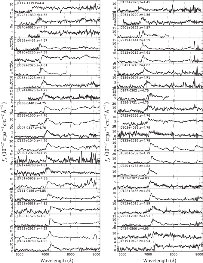
Figure 6. Spectra of 72 newly discovered quasars. We smoothed the spectra by different size boxcars for spectra taken by different instruments. The spectra taken by WiFeS were smoothed to  . The spectra taken by G3 were smoothed to
  . The spectra taken by G5 were smoothed to
  . The MMT/270 gpm spectra were smoothed to
  and
and  for those using the
  and
and  slits, respectively. The spectra taken by R400 were smoothed to
  and the spectra taken by G12 were smoothed to
  . We present the spectra with the nominal flux calibrations obtained from standard star observations and scaled to the SDSS i-band magnitude. The vertical gray lines mark the locations of typical emission lines: in order,
  , Si iv, and C iv.
Download figure:
Standard image High-resolution image4. RESULTS
4.1. Discovery of 72 New Quasars at  5
5

We have spectroscopically observed 99 candidates with z-band magnitudes brighter than 19.5, and 64 (64.6%) of them are quasars with redshifts of  and absolute magnitudes of
  . We also observed 14 fainter candidates selected with the same selection criteria and identified 8 (57.1%) fainter
  quasars with
  and absolute magnitude of
  . Table 4 lists the redshifts and SDSS + WISE photometry of the 72 newly discovered quasars and Figure 5 shows the optical spectra of these new quasars. The redshifts of these quasars were measured from
  , N v, O i/Si ii, C ii, Si iv, and C iv emission lines (any available). We used a visual recognition assistant for quasar spectra software (ASERA; Yuan et al. 2013), which is an interactive semi-automated toolkit allowing the user to visualize observed spectra and measure the redshifts by fitting the observed spectra to the SDSS quasar template (Vanden Berk et al. 2001) and interactively accessing related spectral line information. The redshift error measured based on this method mainly depends on the quality of the observed spectra and line properties. Due to the low resolution and strong absorptions blueward of
  , the typical redshift error is about 0.05 for our newly discovered quasars. However, the redshift error could be up to 0.1 for objects with relatively low S/N spectra. Our quasar sample spans a redshift range of
  and the redshift distribution of these newly identified quasars is shown in the lower panel of Figure 7. As we discussed in Section 2 there is a gap in the previously published quasar redshift distribution at
  with only 33 published quasars at this redshift due to low identification efficiency; 17 of them were identified by the SDSS quasar survey. Among the 72 newly identified quasars, 12 of them are at
  , which represents an increase of ∼36% in the number of known quasars in this difficult redshift range.

Figure 7. Upper panel: the M1450 vs. redshift diagram. The small blue crosses denote SDSS  quasars and the red stars denote our newly discovered quasars. The M1450 are AB magnitudes of quasars at
  . Lower panel: the redshift distributions of newly identified quasars and known
  quasars. Our method improves the completeness of selecting quasars at
  , which is consistent with the prediction from the color-z relation shown in Figure 3. Right panel: the distribution of M1450. Apparently our newly discovered quasars are systematically brighter than SDSS quasars and improved the completeness of luminous
  quasars in the SDSS footprint.
Download figure:
Standard image High-resolution imageTable 4.
Photometry of Four  Quasars Selected by Our Method
| Name | Redshift | m1450 | M1450 | i |

|
z |

|
W1 |

|
W2 |

|
|---|---|---|---|---|---|---|---|---|---|---|---|
| J010013.02+280225.8a | 6.30 ± 0.01 | 17.51 | −29.26 | 20.84 | 0.06 | 18.33 | 0.03 | 14.46 | 0.03 | 13.64 | 0.03 |
| J154552.08+602824.0 | 5.78 ± 0.03 | 19.26 | −27.37 | 21.27 | 0.07 | 19.09 | 0.05 | 16.00 | 0.04 | 15.16 | 0.05 |
| J232514.24+262847.6 | 5.77 ± 0.05 | 19.64 | −26.98 | 21.62 | 0.17 | 19.41 | 0.10 | 16.19 | 0.06 | 15.41 | 0.10 |
| J235632.44–062259.2 | 6.15 ± 0.02 | 19.89 | −26.85 | 22.55 | 0.35 | 19.78 | 0.11 | 16.56 | 0.10 | 15.70 | 0.20 |
Note.
aSee Wu et al. (2015) for details.Download table as: ASCIITypeset image
In Table 3 columns m1450 and M1450 list the apparent and absolute AB magnitudes of the continuum at rest-frame  , respectively. They were calculated by fitting a power-law continuum
  to the spectrum of each quasar. As many spectra of our newly discovered quasars do not have enough continuum coverage to reliably measure the slopes of the continua, we assumed that the slope is consistent with the average quasar UV continuum slope
  (Vanden Berk et al. 2001). The power-law continuum was then normalized to match visually identified continuum windows that contain minimal contribution from quasar emission lines and from sky OH lines. Figure 7 shows the absolute magnitude at rest-frame
  and the redshift distribution of our 72 newly discovered quasars and the published SDSS
  quasars. The red stars are our newly discovered quasars and the blue crosses denote SDSS quasars. The red and blue dashed lines in Figure 7 denote the mean absolute magnitude of our new quasars (
 ) and the SDSS quasars (
 ), respectively. Our newly discovered quasars are systematically brighter than SDSS quasars and improved the completeness of luminous
  quasars in the SDSS footprint. More importantly, 24 of our newly discovered quasars have
  and doubled the number of known quasars (26
  SDSS quasars) in this brightness range in the SDSS footprint. In particular, 22 of our new quasars are at
  with
with  compared with only 13 previously published SDSS quasars in this redshift/luminosity range.
4.2. Notes on Individual Objects
SDSS J013127.34–032100.1 (z = 5.19). The radio loudness defined as the ratio of the rest-frame flux densities in the radio (5 GHz) to optical bands (4400 Å) bands (Kellermann et al. 1989). J0131–0321 is a radio-loud quasar with radio loudness of about 100. J0131–0321 is the most luminous  radio-loud quasar known, with a SDSS z-band magnitude of 18.01 ± 0.03 and with
  . The observational properties of this quasar are discussed in detail in a separate paper (Yi et al. 2014).
SDSS J022112.62–034252.26 (z = 5.02). J0221–0342 was independently discovered by the BOSS quasar survey and published in the DR12 quasar catalog (I. Pâris et al. 2016, in preparation).
SDSS J030642.51+185315.8 (z = 5.36). J0306+1853 is the most luminous  quasar known to date, with
  . A more detailed analysis of this quasar is in Wang et al. (2015).
SDSS J220710.12–041656.28 (z = 5.53). J2207–0416 is the most distant quasar discovered in our  main sample. Note that due to the extremely similar optical-to-IR colors of
  quasars and M dwarfs, there are only two known
  quasars published before: RD J030117+002025 at z = 5.50 (Stern et al. 2000) and NDWFS J142729.7+352209 at z = 5.53 (Cool et al. 2006).
5. DISCUSSION
5.1. Comparison with SDSS Quasar Selection

The SDSS quasar surveys provided the largest quasar sample selected based on SDSS  photometry and have discovered ∼500 quasars at
  (e.g., Schneider et al. 2010; Pâris et al. 2012, 2014). The primary method for selecting
  quasars in the SDSS quasar surveys is based on the
  color–color diagram (Fan et al. 1999; Richards et al. 2002). Since the third stage of the SDSS (BOSS) high-redshift quasar survey mainly focused on fainter targets, here we compare our selection only to the first two stages of SDSS high-redshift quasar selection. There are 392
  quasars in the SDSS DR7 quasar catalog (Schneider et al. 2010). Three hundred and fifty-six of them have counterparts within 2'' in the ALLWISE catalog and 126 (32%) of them satisfy our selection criteria (also including those with z-band magnitudes fainter than 19.5). Figure 8 shows 392 SDSS high-z quasars: red circles denote quasars that satisfy our selection criteria and blue crosses denote quasars that do not satisfy our selection criteria. Clearly quasars that are not selected by our method are mainly objects with
  quasars or with fainter magnitudes. As Figure 3 shows, about 60% of quasars at
  have W1–W2
  which is the reason why our method is not sensitive to
  quasars.

Figure 8. Redshift vs. z-band magnitude diagram of SDSS DR7  quasars. The red circles denote quasars that satisfy our selection method while blue crosses denote quasars that do not satisfy our selection method. The purple line represents z-band magnitudes equal to 19.5.
Download figure:
Standard image High-resolution imageAll our targets are within the SDSS footprint, therefore we examined the 72 newly discovered quasars against the SDSS high-redshift quasar selection criteria presented in Richards et al. (2002). There are three reasons that they are not in the SDSS quasar catalogs: (1) 38 of them are not in the SDSS DR7 photometry sky coverage and thus not in the SDSS main spectroscopy survey region; (2) 25 new quasars have the quasar target flag set by the latest SDSS target selection pipeline but were not observed either because these candidates are at the edge of SDSS main spectroscopy survey or the fields of these candidates were observed at the early stage of the SDSS (e.g., SDSS EDR and DR1) when a preliminary version of the selection pipeline was used (Richards et al. 2002), and (3) The other nine new quasars were not targeted by SDSS altogether. These nine quasars were rejected by the photometric flags (e.g., BLENDED, INTERP_CENTER, CHILD, and FAMILY). Although the SDSS high-redshift quasar target selection method can recover many of these newly discovered quasars, the efficiency (less than 10%) of the SDSS target selection is much lower than that (∼60%) of our method by combining SDSS and ALLWISE colors. In addition, our method improved both the completeness and efficiency for selecting  quasars (the region between the purple dashed line and the orange dashed line in Figure 4).
5.2. Efficiency and Completeness of Our Quasar Selection
In our spectroscopic observations ∼60% of our candidates are real high-redshift quasars, which is a relatively high efficiency for selecting high-redshift quasars. Although our optical color cuts are very sensitive to  (Figure 4), quasars at
  have a bluer W1–W2 color and lead to a lower completeness of our selection method in this redshift range (Figures 3 and 8). At
  , the WISE W1 and W2 bands only cover quasar rest-frame optical emission (shorter than
  m), which is not significantly polluted by the hot dust (e.g., Leipski et al. 2014). The W1–W2 color changes a lot from redshift 4.5 to 5.5 as the
  emission line moves from W1 to W2. More than half of the quasars at
  have a bluer W1–W2 with W1–W2
  . At this redshift range, the
  emission line redshifts into the W1 band. Quasars with weaker
  emission lines or a redder continuum will prefer redder W1–W2 colors and quasars with stronger
  emission lines or a bluer continuum will show bluer W1–W2 colors. So our W1–W2 cut will bias to quasars with weaker
  emissions or a redder continuum at
  . At
. At  the
the  emission line moves out from W1 band and the W1–W2 colors change to be redder and our W1–W2 cut will not bias to quasars emission line and continuum properties significantly. Overall, our selection method can select luminous quasars at
  with both high efficiency and relatively high completeness (e.g., Figure 7). Benefiting from this we will be able to study the QLF at
  , especially at the bright end of the QLF, and do detailed statistics on quasar properties based on a complete sample of SDSS–WISE selected
  quasars in the near future (J. Yang et al. 2016, in preparation). More detailed analysis of the completeness of our quasar sample will be discussed in the QLF paper.
Although ALLWISE has whole-sky coverage, SDSS is limited to only one quarter of the sky. New optical sky surveys are providing coverage of the entire high galactic latitude sky: the PAN-STARRS-1 survey (Kaiser et al. 2002, 2010) has a much larger sky coverage and a slightly deeper depth in red filters than SDSS and it has a y-band filter that covers the  range, allowing quasar selection to
  . Combining PAN-STARRS with ALLWISE photometry will provide a much more comprehensive way to find luminous high-redshift quasars. Many other ongoing large-area optical sky surveys including SkyMapper, VST ATLAS, DECaLS, BASS, and DES will enable a complete all-sky survey of luminous high-redshift quasars by combining them with the ALLWISE photometry.
6. OPTICAL SURVEYS PLUS WISE FOR FINDING LUMINOUS z ≳ 5.7 QUASARS
As Figure 3 shows, quasars at  have relatively redder W1–W2 colors which are useful for rejecting late-type star contamination. Figure 9 shows the known
  quasars (Table 1 and references therein) and M, L, and T dwarfs (Kirkpatrick et al. 2011) on the
  W1/W1–W2 color–color diagram. The cyan cycles denote
  quasars, the blue triangles represent
  quasars, and the orange stars represent
  quasars. Clearly the optical plus WISE photometric selection method can separate quasars from contaminants at redshifts up to
  , the upper redshift limit of optical surveys. However, the L and T dwarfs begin to overlap with
  quasars in this color–color diagram which is a limit for finding quasars at this redshift range. It could be improved by combining near-infrared photometry (e.g., Y-band and J-band) as L and T dwarfs have redder Y − J colors than that of
  quasars (Venemans et al. 2013). Actually, Carnall et al. (2015) have used a similar method (
 W2/W1–W2) to search for
  quasars in the VST ATLAS survey and have identified two new
  luminous quasars in the ATLAS survey area.

Figure 9.  W1 vs. W1–W2 color–color diagram. The green solid line represents the color-z relation predicted using quasar composite spectra. The green solid squares mark the color tracks for quasars from z = 5.0 to z = 7.0 in steps of
  . The cyan circles denote
  quasars, the blue triangles denote
  quasars, and the orange stars denote
  quasars. The red stars represent our four newly discovered z ≳ 5.7 quasars. The black crosses, open triangles, and open squares are M, L, and T dwarfs, respectively, from Kirkpatrick et al. (2011).
Download figure:
Standard image High-resolution imageMotivated by the high detection rate of luminous high-redshift quasars as described in Section 2 (e.g.,  at
at  and
and  at
at  ), we also search for luminous z ≳ 5.7 quasars by combining the i-dropout technique (e.g., Fan et al. 2001b; Willott et al. 2007; Jiang et al. 2008; Bañados et al. 2014) and
  W1/W1–W2 colors mentioned above. This method can be used to reject superposed objects without any photometric followup observations and can reject the majority of contaminants (mainly L and T dwarfs). We selected about 20 i-dropouts with
  in the SDSS area. Before doing spectroscopy we visually compared the spectra energy distribution (SED) of these candidates with type 1 quasar composite SED (Richards et al. 2006) to rank the priority.
We have observed four candidates with the highest priority and have identified four z ≳ 5.7 quasars: J010013.02+280225.8 at  (Wu et al. 2015), J235632.44–062259.2 at
  , J154552.08+602824.0 at
  , and J232514.24+262847.6 at
  . Table 4 lists the photometric and redshift information for these four quasars and Figure 10 shows their optical spectra. The spectrum of J0100+2802 was obtained with LBT/MODS spectrograph (Pogge et al. 2010) and the redshift determined from Mg ii emission line in the near-IR spectrum (Wu et al. 2015). J0100+2802 is the most luminous
  quasar ever known and hosts a 12 billion solar black hole in its center (Wu et al. 2015). We observed J1545+6028 with the G5 grating on the LJT 2.4 m telescope with a 3600-s exposure on 2014 April 5. This quasar was not targeted by SDSS main z ∼ 6 quasar survey as its
  does not satisfy their i − z cut (Fan et al. 2001a). The spectrum of J2325+2628 was obtained with MMT Red Channel on 2015 May 9. We used the 27 gpm grating centered at
  and a
and a  slit. The MMT spectrum shows that J2325+2628 is a weak-line emission quasar (WLQ) and with the current S/N there are no clear emission lines. The redshift of J2325+2628 was estimated by fitting the continuum to the composite spectra (Vanden Berk et al. 2001). Although this quasar has SDSS photometry data and satisfy SDSS z ≳ 5.7 selection criteria, it does not fall in the SDSS z ≳ 5.7 quasar survey region. We observed J2356–0622 with ANU WiFeS with a 30-minute exposure on 2015 May 15. However, the target was only marginally detected due to the cloudy weather and it was hard to confirm that it is a high-redshift quasar. A further one-hour exposure was obtained with WiFeS on 20 July, which confirmed J2356–0622 as a quasar at z = 6.15. J2356–0622 is the faintest
  quasar in our sample with
  . This quasar has a bad SDSS photometry flag (maybe a cosmic ray) and was not selected by SDSS. The redshifts of J1545+6028 and J2356–0622 were determined by using ASERA to visually fit the
  , N v emission lines, and the position of
  drop.
drop.

Figure 10. Optical spectra of four z ≳ 5.7 quasars discovered by using the method described in Section 6. J0100+2802 is the most luminous quasar at  known to date and has been reported in Wu et al. (2015).
Download figure:
Standard image High-resolution image
Although we have identified four z ∼ 6 quasars with our method, we still cannot give an accurate success rate for finding z ≳ 5.7 quasars as we only observed very few candidates with highest priority. We are still working on the spectroscopy observations and will also extend our method to the ongoing DECam legacy survey (DECaLS) and the unblurred coadds of the WISE Imaging (unWISE; Lang 2014) to find fainter z ≳ 5.7 quasars.
7. SUMMARY
The SDSS spectroscopic surveys have discovered the majority of quasars known to date. However, they have a lower degree of completeness at high redshift (e.g.,  ). Even with additional efforts aimed at finding high-redshift quasars by using SDSS and other photometric data (e.g., Fan et al. 1999, 2000b; Willott et al. 2007; Jiang et al. 2008; Mortlock et al. 2011; McGreer et al. 2013; Venemans et al. 2013), there is an obvious gap for quasars at
  . Up to now about 300,000 quasars have been spectroscopically identified, but only ∼700 quasars at
  , ∼ 30 quasars at
  and ∼90 quasars at
  .
.
ALLWISE has a high detection rate of known high-redshift quasars, especially in the two bluest WISE bands. The W1–W2 color can be used to reject late-type stars efficiently. We have developed a new method by combining optical and WISE colors that yields a much higher selection efficiency for finding luminous high-redshift quasars than by using only optical colors. We have assembled a sample of  quasar candidates using SDSS and ALLWISE photometric data and have spectroscopically identified 72 new
  quasars, with 12 quasars at
  , allowing us to begin filling the gap at
  . Our current spectroscopic observations have led to an increase of ∼36% of quasars at
  . However, this gap is still far from being filled as our method only focus on quasars at
  . A lot of work still needs to be done to find more quasars at this redshift range. Our new quasar sample is about 0.8 mag brighter than SDSS
  quasars and is expected to set strong constraints on the bright end of the
  QLF (J. Yang et al. 2016, in preparation; Paper II), the massive end of the BHMF with future near-IR spectroscopy (Paper III), and the high-redshift IGM through future high-resolution quasar absorption spectra. Moreover, our method can also be used to find quasars with redshifts up to
  and we have identified four quasars with redshifts beyond 5.7.
F. W. and X-B. W. thank the support from the NSFC grants No.11373008 and 11533001, the Strategic Priority Research Program "The Emergence of Cosmological Structures" of the Chinese Academy of Sciences, grant No. XDB09000000, and the National Key Basic Research Program of China 2014CB845700. F. W. thanks the financial support from the program of China Scholarships Council No. 201406010031 during his visit to the University of Arizona. X. F. and I. D. M. thank the support from the US NSF grant AST 11-07682. This research uses data obtained through the Telescope Access Program (TAP), which has been funded by the Strategic Priority Research Program "The Emergence of Cosmological Structures" (grant No. XDB09000000), National Astronomical Observatories, Chinese Academy of Sciences, and the Special Fund for Astronomy from the Ministry of Finance. We acknowledge the support of the staff of the Lijiang 2.4 m telescope. Funding for the telescope has been provided by CAS and the People's Government of Yunnan Province. We acknowledge the use of the MMT Observatory, a joint facility of the Smithsonian Institution and the University of Arizona. We acknowledge the use of the Bok telescope and ANU 2.3 m telescope. We acknowledge the use of Xinglong 2.16 m telescope. This work was partially supported by the Open Project Program of the Key Laboratory of Optical Astronomy, National Astronomical Observatories, Chinese Academy of Sciences.
We acknowledge the use of SDSS photometric data. Funding for SDSS-III has been provided by the Alfred P. Sloan Foundation, the Participating Institutions of the SDSS, the National Science Foundation, and the U.S. Department of Energy Office of Science. The SDSS-III Web site is http://www.sdss3.org/. SDSS-III is managed by the Astrophysical Research Consortium for the Participating Institutions of the SDSS-III Collaboration including the University of Arizona, the Brazilian Participation Group, Brookhaven National Laboratory, the University of Cambridge, Carnegie Mellon University, the University of Florida, the French Participation Group, the German Participation Group, Harvard University, the Instituto de Astrofisica de Canarias, the Michigan State/Notre Dame/JINA Participation Group, Johns Hopkins University, the Lawrence Berkeley National Laboratory, the Max Planck Institute for Astrophysics, the Max Planck Institute for Extraterrestrial Physics, New Mexico State University, New York University, Ohio State University, the Pennsylvania State University, the University of Portsmouth, Princeton University, the Spanish Participation Group, the University of Tokyo, the University of Utah, Vanderbilt University, the University of Virginia, the University of Washington, and Yale University. This publication makes use of data products from the Wide-field Infrared Survey Explorer, which is a joint project of the University of California, Los Angeles, and the Jet Propulsion Laboratory/California Institute of Technology as well as NEOWISE, which is a project of the Jet Propulsion Laboratory/California Institute of Technology. WISE and NEOWISE are funded by the National Aeronautics and Space Administration.
Facilities: Sloan (SDSS) - , WISE - Wide-field Infrared Survey Explorer, 2.4 m/YNAO (YFOSC) - , MMT (Red Channel spectrograph) - , 2.16 m/NAOC (BFOSC) - , 2.3 m/ANU (WiFeS) - .
Footnotes
- 11
- 12
- 13
- 14
- 15