


ABSTRACT
Globular clusters are of paramount importance for testing theories of stellar evolution and early galaxy formation. Strong evidence for multiple populations of stars in globular clusters derives from observed abundance anomalies. A puzzling example is the recently detected Mg–K anticorrelation in NGC 2419. We perform Monte Carlo nuclear reaction network calculations to constrain the temperature–density conditions that gave rise to the elemental abundances observed in this elusive cluster. We find a correlation between stellar temperature and density values that provide a satisfactory match between simulated and observed abundances in NGC 2419 for all relevant elements (Mg, Si, K, Ca, Sc, Ti, and V). Except at the highest densities (ρ ≳ 108 g cm−3), the acceptable conditions range from ≈100 MK at ≈108 g cm−3 to ≈200 MK at ≈10−4 g cm−3. This result accounts for uncertainties in nuclear reaction rates and variations in the assumed initial composition. We review hydrogen-burning sites and find that low-mass stars, asymptotic giant branch (AGB) stars, massive stars, or supermassive stars cannot account for the observed abundance anomalies in NGC 2419. Super-AGB stars could be viable candidates for the polluter stars if stellar model parameters can be fine-tuned to produce higher temperatures. Novae, involving either CO or ONe white dwarfs, could be interesting polluter candidates, but a current lack of low-metallicity nova models precludes firmer conclusions. We also discuss whether additional constraints for the first-generation polluters can be obtained by future measurements of oxygen, or by evolving models of second-generation low-mass stars with a non-canonical initial composition.
Export citation and abstract BibTeX RIS
1. INTRODUCTION
Globular clusters represent fascinating puzzles, particularly since it was discovered that they consist of multiple populations of stars. Distinct populations within a given globular cluster manifest themselves by discrete tracks in the color–magnitude diagram (Piotto et al. 2007; Villanova et al. 2007) and a negative correlation (anticorrelation) of abundances between pairs of light elements, such as C–N, O–Na, and Mg–Al. For a recent review, see Gratton et al. (2012). Since the anticorrelations are mostly absent7 in halo field stars (Gratton et al. 2000), their origin must be related to the poorly understood processes of globular-cluster and early galaxy formation.
The abundance anticorrelations have been detected both in red giants and in unevolved stars (Gratton et al. 2001). Since these low-mass stars cannot produce the high temperatures required to alter the abundances of O, Na, Mg, or Al (Powell et al. 1999; Gratton et al. 2004), the reported abundance anomalies likely originate from an earlier (i.e., first-generation globular cluster) stellar population that subsequently polluted the matter out of which the currently observed second-generation globular cluster stars formed.8 The latter stars presumably formed in a dense environment occupied by the first-generation stars. The observations confront us with a number of crucial questions. How many star-forming episodes took place in globular clusters? How does the process of star formation in a dense cluster environment differ from that in a molecular cloud devoid of stars? What kind of first-generation stars gave rise to the abundance anticorrelations and what was their composition?
The measured abundance anticorrelations differ in magnitude from cluster to cluster, even among the clusters that show no significant spread in the iron content. The Mg–Al anticorrelation, for example, is not observed in some globular clusters. This suggests that the pollution mechanism and the nature of the polluter stars (also called polluters) may vary, depending on the total mass and metallicity of the cluster (Carretta et al. 2009; Meszaros et al. 2015).
For the cluster NGC 6752, the measured stellar abundance anomalies involving O, Na, Mg, and Al can be explained by hydrogen burning at moderate temperatures, near 75 MK, as was shown by Prantzos et al. (2007). Candidate sources for the first-generation polluter stars include rapidly rotating massive stars (Decressin et al. 2007), massive stars in interacting binary systems (de Mink et al. 2009), stellar collisions (Sills & Glebbeek 2010), supermassive stars with M ≈ 104 M⊙ (Denissenkov & Hartwick 2014), intermediate-mass asymptotic giant branch (AGB) stars (D'Antona et al. 2002), super-asymptotic giant branch (SAGB) stars (Ventura et al. 2012), and novae (Smith & Kraft 1996; Maccarone & Zurek 2012), but detailed stellar models fail to account for all observations.
The recent discovery of a Mg–K anticorrelation among red giant stars in the cluster NGC 2419 (Cohen & Kirby 2012; Mucciarelli et al. 2012) adds to the mystery of abundance anomalies in globular clusters. The strong potassium enhancements, correlated with magnesium depletions, cannot be explained by hydrogen burning at moderate temperatures, near 75 MK, where the Coulomb barrier gives rise to insufficiently small thermonuclear rates of the relevant proton capture reactions. Elevated temperatures will be required to account for the reported potassium enhancements. Recently, potassium enhancements have also been measured in NGC 2808 (Mucciarelli et al. 2015), albeit of a much smaller magnitude.
The nature and origin of the metal-poor cluster NGC 2419 are not yet understood. It is located in the outer halo, further away than the Small and Large Magellanic clouds, at a galactocentric distance of 87.5 kpc. It is 12.3 ± 1.3 Gyr old (Forbes & Bridges 2010) and has an orbital period of about 3 Gyr (Di Criscienzo et al. 2011). It is the third most massive cluster (9.12 × 10⁵ M⊙; Ibata et al. 2011a) in our Galaxy. For a massive globular cluster, it also has an unusually large half-light radius of 24 pc (Ibata et al. 2011b). Therefore, it was suggested that NGC 2419 may not be a genuine globular cluster, but rather the remnant of an accreted dwarf galaxy (Mackey & van den Bergh 2005). The recently observed strong potassium enhancements contribute to the puzzle surrounding this stellar aggregate.
A first attempt to explain the measured strong potassium abundance enhancements that are correlated with large magnesium depletions in the atmospheres of red giants in NGC 2419 was made by Ventura et al. (2012). They assumed that the anomalous abundances are produced during hot-bottom burning in massive AGB stars and super-AGB stars, involving temperatures near 150 MK, and that the second-generation stars formed directly from the ejecta of the first-generation AGB or super-AGB stars. However, a number of parameters, such as thermonuclear reaction rates and the stellar mass loss rate, had to be fine-tuned in their models to account for the reported Mg–K anticorrelation.
We do not know the nature of the first-generation polluter stars that gave rise to the reported abundance anomalies in the currently observed second generation. In this work, we will provide a fresh look at this puzzling situation. We choose not to limit ourselves to specific stellar models but will perform nuclear reaction network calculations at constant temperature, T, density, ρ, amount of consumed hydrogen, ΔXH, and initial composition, Xi, following broadly the ideas presented in Prantzos et al. (2007). These parameters are varied in a Monte Carlo procedure to determine the conditions that best reproduce not only the reported Mg–K anticorrelation but all relevant observed abundances in NGC 2419. This information will be important for identifying the astrophysical sites that gave rise to the puzzling abundance anomalies. The results could have significant implications for models of both stellar and globular cluster formation.
In Section 2 we discuss our procedure in more detail, including the observations, our nuclear reaction network, the assumed initial composition, and the nucleosynthesis during hydrogen burning. Results are presented in Section 3. Candidate sources for first-generation polluter stars are discussed in Section 4. In Section 5, we comment on possibilities to further constrain the conditions in the polluter candidates. A summary and conclusions are given in Section 6.
2. PROCEDURE
2.1. General Considerations
The scenarios of globular cluster formation and evolution are shown schematically in Figure 1. After primordial nucleosynthesis (a)–(b), the first stars form (b). The ejecta and winds of these zero-metallicity stars, including the contributions from massive stars of subsequent generations, enrich the proto-cluster gas with metals (c). Eventually, the first-generation globular cluster stars form (d). The massive stars among these evolve quickly and explode as type II supernovae. Other first-generation stars (1) undergo hydrogen burning during their evolution, giving rise to the ubiquitous O–Na anticorrelation that we observe in second-generation stars. We will call the process responsible for the anomalous CNO, Na, Mg, and Al abundance pattern low-temperature hydrogen burning (LTB). Other first-generation stars (2), or the same ones (3), undergo hydrogen burning at higher temperatures, giving rise to the recently discovered Mg–K anticorrelation. We refer to this process as high-temperature hydrogen burning (HTB). During their evolution, the first-generation stars eject part of their matter (e). The currently observed second-generation stars form from the polluted intracluster gas (f), thereby inheriting the nucleosynthesis signatures of both the pre-enrichment before cluster formation and the first-generation stars (see, e.g., Decressin et al. 2008; D'Ercole et al. 2008). Today (g), globular clusters consist mainly of old, low-mass stars and very little cold gas.

Figure 1. Schematic representation of globular cluster evolution: (a) Big Bang; (b) zero-metallicity stars form; (c) type II supernovae enrich the proto-cluster gas; (d) birth of first-generation globular cluster stars: some may undergo low-temperature hydrogen burning (LTB) only (1), high-temperature hydrogen burning (HTB) only (2), or undergo both processes at different times (3); (e) pollution of the intracluster medium (ICM) by first-generation stars; (f) second-generation stars form and evolve until the present time (g). The time axis is not to scale: the time between first- and second-generation star formation, (d)–(f), is ≲1.0 Gyr, whereas the age of an old cluster, (a)–(g), is >10 Gyr.
Download figure:
Standard image High-resolution imageThe above picture is broadly supported by observations. For most globular clusters, the Fe-group elements (Fe, Cu, Ni), α-elements (e.g., Si, Ca), s-process abundances (e.g., Ba, Sr), and r-process abundances (e.g., Eu) in a given cluster scatter little from star to star and are independent of the evolutionary phase of the observed globular cluster stars (James et al. 2004). This indicates that the globular cluster formed from pre-enriched homogeneous matter. Furthermore, the abundances of the light metals (i.e., C to K) are not correlated with those of the heavy metals (i.e., iron peak, s-process, and r-process elements), indicating that the site responsible for the light-element abundance anomalies did not produce significant amounts of Fe, s-process, and r-process elements (James et al. 2004; Prantzos & Charbonnel 2006). This argues strongly against type II supernovae as the first-generation polluters.
An important step in identifying the polluters is to constrain the physical conditions for hydrogen burning that gave rise to the abundance anomalies. For the well-studied cluster NGC 6752, Prantzos et al. (2007) applied a simple method that did not depend on any specific stellar model. The method has the additional advantage of making robust predictions once the necessary thermonuclear reaction rates are reliably known. They performed a series of hydrogen-burning reaction network simulations at constant temperature and density, for a given amount of consumed hydrogen, and identified the conditions that simultaneously reproduced all of the measured light-element abundances, from C to Al. Each network simulation started from an initial composition obtained from observations of field stars with a similar iron content to NGC 6752. It was found that a narrow temperature range around 75 MK could account for the light-element anomalies, if the nuclearly processed matter is mixed with at least 30% of pristine (i.e., unprocessed) matter. The reported anomalies, including the ubiquitous O–Na anticorrelation, are then reproduced, assuming a range of mixing (or dilution) factors in excess of 30%. They also suggested stellar sites for this low-temperature hydrogen burning, including AGB stars and fast rotating massive stars, but detailed stellar models for both sites have difficulties accounting for the observations (Gratton et al. 2012). We will apply a similar model to investigate the abundance pattern of light elements measured in NGC 2419 (Cohen & Kirby 2012; Mucciarelli et al. 2012).
2.2. Observations in NGC 2419
The stars in NGC 2419 have an average metallicity of [Fe/H] = −2.09 ± 0.029 , with no intrinsic spread in the iron abundance (Cohen & Kirby 2012; Mucciarelli et al. 2012). Measured elemental abundances versus potassium abundance for red giants in NGC 2419 are shown as data points in Figure 2. The red and blue data points are adopted from Mucciarelli et al. (2012) and Cohen & Kirby (2012), respectively. All abundances were derived from a local thermodynamic equilibrium (LTE) analysis using one-dimensional model atmospheres. The sole exception is the potassium abundance reported by Mucciarelli et al. (2012), who applied a unique value of −0.3 dex for the non-LTE correction to all targets. We decided to adopt all reported abundances at face value, as was done in other work (Bellazzini et al. 2013; Ventura et al. 2012). Attempting to place the two studies onto the same scale is not trivial, given their differences in spectral resolution, analysis technique, application of uniform NLTE corrections, and adopted solar abundance.
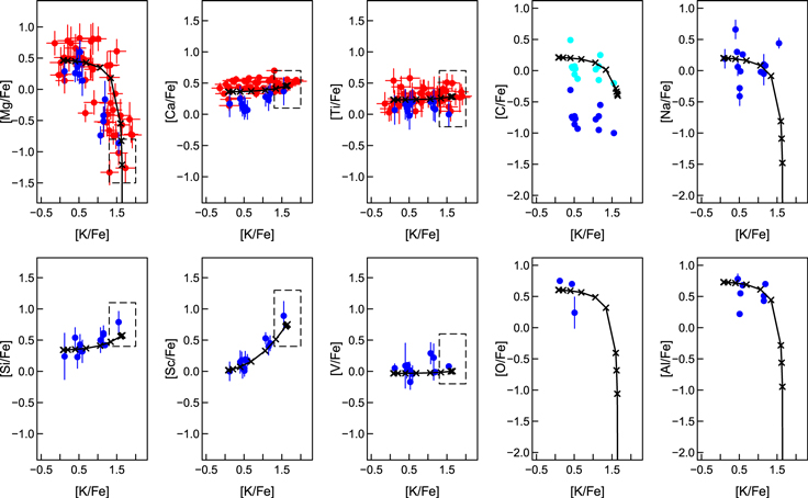
Figure 2. Elemental abundances, with respect to Fe, vs. K abundance for red giants in NGC 2419. Red: observations of Mucciarelli et al. (2012); dark blue: observations of Cohen & Kirby (2012); light blue: from Cohen & Kirby (2012), but 0.8 dex was added to [C/Fe] (see text). Simulations are shown in black for the conditions T = 160 MK, ρ = 900 g cm−3, and  = 0.70: the solid lines are obtained by mixing one part of processed matter with f parts of pristine matter, according to Equation (1); the crosses on the solid lines denote, from left to right, the abundances obtained with dilution factors of f = 1000, 100, 30, 10, 3, 1.0, 0.1, 0.05, 0.02, and 0.0. In some panels, the cross for f = 0.0 is off the scale. The pristine matter composition (on the left-hand side) is fixed by the initial abundances listed in Table 1, while the (undiluted) processed matter composition (on the right-hand side) is given by the output of the reaction network calculation. The range of acceptable processed abundances is indicated by the dashed boxes.
Download figure:
Standard image High-resolution imageThe first panel shows the Mg–K anticorrelation: when the K abundance is low, the Mg abundance is high (Mg-normal); when K is strongly enhanced (by ≈1.5 dex), Mg is strongly depleted (by ≈2.0 dex). Notice that about 30% of the observed red giants show strong potassium enhancements. In other words, about 30% of the stars in NGC 2419 consist of matter that underwent an unknown process.
Both Si and Sc show an increase in abundance for the K-enhanced stars, by about 0.5 dex. The abundances of Ca, Ti, and V are approximately constant for a wide range of K abundances. The panels on the right show the abundances of elements in the CNO and Na–Al region: Na and Al reveal no correlation with K, but a large scatter instead; O is only reported in three stars.
Carbon (fourth panel in top row) is the only element shown in Figure 2 whose abundance is affected by the evolution of the second-generation stars we currently observe. Because of the distance of NGC 2419, the red giants with measured carbon are all located at the tip of the red giant branch (see Figure 1 in Cohen & Kirby 2012). If all these observed stars were born with a composition typical for field stars of the same metallicity, they would have depleted C during their evolution from the luminosity function bump to the tip of the red giant branch. For the cluster NGC 2419, with an average metallicity of [Fe/H] = −2.1, the estimated depletion is ≈0.8 dex (Angelou et al. 2012). The expected natal carbon abundance of the currently observed stars, with 0.8 dex added to the measured values, is shown as light blue data points in Figure 2 (fourth panel in top row). We will discuss this assumption further in Section 2.7.
The helium abundance has also been inferred in NGC 2419, both for red giants (Lee et al. 2013) and for horizontal branch stars (Di Criscienzo et al. 2015). We will discuss these observations in Section 5.1.
The second-generation red giant stars that we observe in NGC 2419 are about 12 Gyr old and, consequently, must have formed very early during globular cluster evolution. The time available for the first-generation stars to pollute the intracluster gas out of which the second-generation stars formed is very uncertain, but is probably less than a few hundred million years.
2.3. Strategy
Reaction rates for charged particles are highly sensitive to temperature and density. LTB (T ≈ 75 MK) explains both the O–Na anticorrelation and the Mg–Al anticorrelation in Galactic globular clusters (Prantzos et al. 2007). This temperature range will affect the abundances of the observed elements from C to Al, but not of heavier elements. As we shall see, HTB (T ≳ 80 MK) is necessary to account for the potassium enhancements in NGC 2419. Such elevated temperatures will affect the abundances of the observed elements C, Na, Mg, Al, Si, K, Ca, and Sc.
The sites of low- and high-temperature hydrogen burning have not been identified yet. We do not know if they operated in different first-generation stars, or in the same stars at different locations, or in the same stars at the same location at different times. We also do not know if low-temperature hydrogen burning took place in NGC 2419. Simultaneous observations of oxygen and sodium are only available for three red giants (Cohen & Kirby 2012) and thus a correlation between these two elements cannot be established at present in this globular cluster. If low-temperature hydrogen burning did take place in NGC 2419, its abundance signatures may have been modified by high-temperature hydrogen burning. We will return to this point in Section 5.
In the present work, we will adopt a simple model that is based on the following assumptions: (i) a single-stage, one-zone (high-temperature) hydrogen-burning process in first-generation stars; and (ii) mixing of matter processed by the polluters with pristine, natal matter of the globular cluster. In particular, we would like to determine the conditions of constant temperature, constant density, and the amount of consumed hydrogen required to reproduce the abundance anomalies observed in NGC 2419 and, thereby, constrain the physical conditions of the first-generation polluter stars.
In a reaction network simulation, the amount of consumed fuel (hydrogen) depends on the duration of nucleosynthesis: the longer the reaction network runs, the more hydrogen is consumed. In many realistic scenarios, convection continuously carries fresh fuel into the burning region and also dilutes the abundances of the products of hydrogen burning. This effect lengthens considerably the duration of hydrostatic nuclear burning compared to the one-zone process adopted in the present work that disregards convection. Also, for explosive nuclear burning, we cannot expect that our one-zone simulations reproduce realistic burning times. For these reasons, the constraints we obtain on the amount of consumed hydrogen, or, equivalently, the duration of the nuclear burning, are not meaningful. It is very important, however, to reproduce all the relevant observed abundances for the same amount of consumed hydrogen (see Prantzos et al. 2007). Otherwise, no meaningful conclusions can be drawn on temperature and density constraints.
2.4. Nuclear Reaction Network
Our reaction network consists of 213 nuclides, ranging from p, n, and 4He to 55Cr. Thermonuclear reaction rates are adopted from STARLIB10 (Sallaska et al. 2013). This library has a tabular format that contains reaction rates and rate probability density functions on a grid of temperatures between 10 MK and 10 GK. The probability densities can be used to derive statistically meaningful reaction rate uncertainties at any desired temperature. Most reaction rates important for the present work that are listed in STARLIB, including 36Ar(p,γ)37K, 38Ar(p,γ)39K, 39K(p,γ)40Ca, and 40Ca(p,γ)41Sc, have been computed using a Monte Carlo method, which randomly samples all experimental nuclear physics input parameters (Longland et al. 2010). For a few reactions, such as 37Cl(p,γ)38Ar, 37Ar(p,γ)38K, and 39K(p,α)36Ar, experimental rates are not available yet, and the rates included in STARLIB are adopted from nuclear statistical model calculations using the code TALYS. In such cases, a reaction rate uncertainty factor of 10 is assumed. Most of the important reaction rates for studying hydrogen burning in globular clusters are based on experimental nuclear physics information and provide a reliable foundation for robust predictions.
Stellar weak interaction rates, which depend on both temperature and density, for all species in our network are adopted from Oda et al. (1994) and, if not listed there, from Fuller et al. (1982). The stellar weak decay constants are tabulated at temperatures from T = 10 MK to 30 GK, and densities of ρYe = 10−1011 g cm−3, where Ye denotes the electron mole fraction. For β+- and β−-decays, the stellar decay constants should converge to their respective laboratory values at the grid point of lowest temperature and density. However, this is not the case for electron captures. When network calculations are performed for densities below ρ = 10 g cm−3, we use the values tabulated at the grid point of lowest density (10 g cm−3) for the stellar weak decay constants since it would be inappropriate to adopt the laboratory value under such conditions. The interesting case of 37Ar is discussed in Section 2.5. Radioactive nuclides (13N, 14O, 15O, 17F, etc.) present at the end of a network calculation were assumed to decay to their stable daughter nuclides.
For 26Al, we included five species: the ground state (26Alg), the isomer (26Alm), and three higher-lying excited states. Gamma-ray transitions between all these levels are explicitly included in our network calculation and, therefore, no artificial assumption about the equilibration of 26Al is required (see, e.g., Iliadis et al. 2011). The decay constants for the γ-ray transitions connecting the 26Al levels are listed in STARLIB (for details, see Sallaska et al. 2013). It should be noted that we do not take into account the density dependence of the electron capture decays for 26Alg  26Mg and 26Alm
  26Mg. The first decay is very slow (T1/2 = 7.17 × 10⁵ yr) and is much slower than the competing 26Alg(p,γ)26Si reaction. The second decay proceeds mainly via β+-decay at densities below 107 g cm−3 (Fuller et al. 1980). Therefore, this effect is very small for the purposes of the present work. For all stellar weak interaction rates, we assumed an uncertainty of a factor of 2.
2.5. Abundance Flows in the Ar–K Region
We will now consider the interplay of nuclear interactions that gives rise to the synthesis of potassium for the conditions of main interest here. Starting from the most abundant argon isotope, 36Ar, the main reaction sequence identified by Ventura et al. (2012) is 36Ar(p,γ)37K(e+,ν)37Cl(p,γ)38Ar(p,γ)39K, and this is repeated by Mucciarelli et al. (2015). The notation used by these authors is incorrect, since 37K can neither capture a positron nor decay directly to 37Cl. What the authors presumably meant is the reaction sequence 36Ar(p,γ)37K(β+ν)37Ar(e−,ν)37Cl(p,γ)38Ar(p,γ)39K, where 37K decays via positron emission to 37Ar, and 37Ar decays via electron capture to 37Cl. But this sequence cannot be the main nucleosynthesis path of 39K either. The situation is depicted in Figure 3. The nuclide 37Ar decays via electron capture to 37Cl with a laboratory decay constant of λlab = 2.3 × 10⁻⁷ s−1. Under stellar conditions its decay will depend strongly on the density. For example, at ρ = 10 g cm−3, the stellar decay constant is λstar = 8.5 × 10⁻¹⁰ s−1 (see also Figure 1.18 in Iliadis 2015), which is significantly smaller than the decay constant for the competing 37Ar(p,γ)38K reaction. For increasing density, the decay constant for electron capture increases, but the decay constant for the competing (p,γ) reaction increases as well. In other words, for all conditions of interest here, the main reaction sequence for potassium synthesis is 36Ar(p,γ)37K(β+ν)37Ar(p,γ)38K(β+ν)38Ar(p,γ)39K, which is indicated by the thick arrows in Figure 3. Only a minor contribution is expected from the branch initiated by the electron capture of 37Ar, which is depicted by the thin arrows.

Figure 3. Nuclear interactions leading to the synthesis of potassium. Gray boxes indicate stable nuclides. The thick arrows depict the main production channel, while only a minor contribution is expected from the path indicated by the thin arrows. The reason is the significantly faster 37Ar(p,γ) reaction compared to the competing electron capture of 37Ar.
Download figure:
Standard image High-resolution image2.6. Initial Composition
For the initial composition, we start with the results of a one-zone chemical evolution model for the Milky Way halo, which is an update of Goswami & Prantzos (2000). The model reproduces the reported abundances in field stars of the same average metallicity as NGC 2419 (i.e., [Fe/H] = −2.1, corresponding to Z = 3.3 × 10⁻⁴). Our adopted values are listed in Table 1. Similar results can be found in Kobayashi et al. (2011). In particular, our initial hydrogen and helium mass fractions amount to  = 0.754 and
  = 0.245, respectively.
Table 1. Assumed Initial (pristine) Composition for Present Network Calculations
| Nuclide | Xia | Nuclide | Xia | |
|---|---|---|---|---|
| 1H | 7.54E-01 | 31P | 1.27E-07 | |
| 2H | 3.93E-05 | 32S | 1.64E-05 | |
| 3He | 2.29E-05 | 33S | 1.07E-07 | |
| 4He | 2.45E-01 | 34S | 1.72E-07 | |
| 6Li | 6.54E-12 | 36S | 3.53E-10 | |
| 7Li | 2.27E-09 | 35Cl | 9.58E-08 | |
| 9Be | 2.21E-12 | 37Cl | 1.42E-08 | |
| 10B | 9.62E-12 | 36Ar | 3.79E-06 | |
| 11B | 4.65E-11 | 38Ar | 1.22E-07 | |
| 12C | 2.98E-05 | 40Ar | 1.58E-11 | |
| 13C | 1.38E-07 | 39K | 3.15E-08 | |
| 14N | 7.31E-06 | 40K | 1.39E-10 | |
| 15N | 1.39E-08 | 41K | 4.65E-09 | |
| 16O | 2.19E-04 | 40Ca | 1.15E-06 | |
| 17O | 2.79E-09 | 42Ca | 7.00E-09 | |
| 18O | 1.41E-08 | 43Ca | 1.93E-10 | |
| 19F | 1.22E-09 | 44Ca | 1.06E-08 | |
| 20Ne | 8.08E-06 | 46Ca | 6.96E-13 | |
| 21Ne | 5.59E-09 | 48Ca | 1.94E-08 | |
| 22Ne | 1.32E-07 | 45Sc | 3.30E-10 | |
| 23Na | 4.30E-07 | 46Ti | 8.96E-10 | |
| 24Mg | 1.53E-05 | 47Ti | 1.88E-10 | |
| 25Mg | 5.25E-08 | 48Ti | 3.92E-08 | |
| 26Mg | 5.81E-08 | 49Ti | 9.81E-10 | |
| 27Al | 2.50E-06 | 50Ti | 2.08E-10 | |
| 28Si | 1.28E-05 | 50V | 1.13E-12 | |
| 29Si | 1.49E-07 | 51V | 2.74E-09 | |
| 30Si | 1.15E-07 |
Note.
aMass fractions adopted from a Galactic chemical evolution model (see text) that reproduces measured abundances in field stars of the same average metallicity as NGC 2419 ([Fe/H] = −2.1). Values in bold were adjusted to match observed abundances of red giants in NGC 2419; the original values of the Galactic chemical evolution model were: Xi = 1.14E-07 (23Na), 8.26E-06 (24Mg), 2.58E-07 (27Al), 3.08E-05 (28Si), 7.15E-08 (39K), 1.85E-06 (40Ca), and 1.54E-09 (51V).Download table as: ASCIITypeset image
The measured abundances of red giants in NGC 2419 (see Section 2.2) provide additional information on the initial composition. Specifically, the stars that do not show any K enhancement and Mg depletion are located on the leftmost side in each panel of Figure 2, near [K/Fe] ≈ 0. These stars are not polluted by material that underwent high-temperature hydrogen burning in the previous stellar generation and, therefore, their abundances can be used to constrain the initial composition of the first-generation stars. The abundance values that we matched to the observations in NGC 2419 are shown in boldface in Table 1, and the corresponding original values predicted by the chemical evolution model are listed in the table footnote. The few adjustments are on the level of factors of 2–3. The only exception was 27Al, whose abundance had to be increased by a factor of ≈10 to match the observations. Notice that the halo model of Goswami & Prantzos (2000) significantly underpredicts the aluminum abundance measured in halo stars at a metallicity of [Fe/H] = −2.1 (see their Figure 7 and Figure 4 in Andrievsky et al. 2008). However, we verified that a variation of the initial 27Al abundance by an order of magnitude up or down had no impact on our results.
2.7. Criteria for Acceptable Solutions
Consider again the measured elemental abundances displayed in Figure 2. Stars with normal Mg and K abundances are shown on the left side in each panel. Their elemental abundances (i.e., pristine matter, defined as the composition of the proto-globular cluster gas; Section 2.1) are in the range of values predicted by models of Galactic chemical evolution (Section 2.6 and Table 1). Stars with the most extreme abundance anomalies are located on the rightmost part in each panel of Figure 2, near [K/Fe] ≈ 2. The first panel shows the Mg abundance declining by two orders of magnitude with increasing K abundance. Even a small amount of mixing with pristine matter would strongly enhance the Mg abundance, and therefore the observed extreme values most likely reflect the nearly undiluted composition (i.e., processed matter) ejected by the polluters. We are seeking the conditions of constant temperature and density that best reproduce these extreme abundance values. Abundances between the pristine and processed matter compositions are obtained in our model by mixing one part of processed matter with f parts of pristine matter. The dilution factors, f, are defined by
where Xproc and Xpris denote the mass fractions of the reaction network output (i.e., processed matter) and the initial composition (i.e., pristine matter), respectively. We are also seeking the dilution factors that best reproduce the measured extreme abundance values.
The dashed boxes on the right-hand side of some panels in Figure 2 show the ranges of acceptable elemental abundances that we impose on the reaction network output. The boundaries indicated by the dashed boxes are given by 1.3 < [K/Fe] < 2.0, −1.5 < [Mg/Fe] < −0.8, 0.1 < [Ca/Fe] < 0.7, −0.2 < [Ti/Fe] < 0.7, 0.4 < [Si/Fe] < 1.1, 0.4 < [Sc/Fe] < 1.3, and −0.2 < [V/Fe] < 0.6. These values are approximations that take into account both the scatter in the data and the abundance uncertainties of individual stars.
For several reasons, we did not impose any boundaries on the carbon abundance. First, carbon may take part not only in hydrogen burning, but also in other burning episodes of the (first-generation) polluters. For example, in AGB and super-AGB stars of low metallicity (Z ≈ 10−4), carbon is produced during thermal pulses (i.e., helium burning) and destroyed during hot-bottom (i.e., hydrogen) burning during the interpulse period (Section 4.3). Whether or not there is a net production of carbon depends on the details of the stellar models (Siess 2010; Doherty et al. 2014). Second, we already noted in Section 2.2 that if all of the observed (second-generation) red giants in NGC 2419 were born with a composition typical for field stars of the same metallicity, they would have depleted C during their evolution from the luminosity function bump to the tip of the red giant branch. Correcting the observations (dark blue data points in the fourth panel of the top row in Figure 2) for this depletion, we obtained the light blue data points, shown in the same panel. This assumption applies to the K-normal stars (i.e., on the left-hand side in each panel of Figure 2), but may not be correct for the extreme stars (i.e., on the right-hand side). Since the latter stars were born from matter that underwent an unknown high-temperature hydrogen burning process, their natal abundances are likely different from those of field stars. We will return to this point in Section 5.
No other observations of stars in NGC 2419 were used as constraints. In particular, it would be dangerous to impose constraints on Na and Al (panels in the last column), since the abundances of these two elements show a significant scatter and no obvious trend with respect to [K/Fe]. As will be seen below, the network calculations that give acceptable solutions within the boundaries listed above will also provide satisfactory fits to the measured Na and Al abundances. The sodium abundance will be discussed in more detail in Section 5.4.
3. RESULTS
3.1. Trial-and-error Solutions
As already pointed out in Section 2.3, the parameters of our model are: (i) constant temperature, T, (ii) constant density, ρ, and (iii) final mass fraction of hydrogen,  =
=  , where
  and ΔXH are the initial and consumed hydrogen abundance, respectively. Besides these parameters, we can also vary the initial composition, Xi, and the thermonuclear reaction rates,
  . We started with a (fixed) initial composition, given in Table 1, and the (fixed) recommended reaction rates listed in STARLIB. The parameters T, ρ, and
  were then varied by trial and error to see if an acceptable fit to all measured abundances could be obtained.
For example, the solid black lines shown in Figure 2 were obtained for the conditions T = 160 MK, ρ = 900 g cm−3, and  = 0.70. The crosses on the black lines denote, from left to right, the abundances obtained with dilution factors of f = 1000 (i.e., almost purely pristine matter), 100, 30, 10, 3, 1.0, 0.1, 0.05, 0.02, and 0.0 (i.e., purely processed matter). The simulated processed abundances (on the right-hand side in each panel) satisfy all of the conditions we imposed for Mg, Si, K, Ca, Sc, Ti, and V (indicated by the dashed boxes). At the same time, this particular solution also approximately reproduces the observations for C, O, Na, and Al. Given our best guess of an initial composition and recommended thermonuclear reaction rates, our first main result is that certain combinations of values of constant temperature, density, and consumed hydrogen mass fraction give a satisfactory fit to the abundances of all the relevant elements observed in NGC 2419. We will next present the results from an automated search.
3.2. Monte Carlo Sampling: Temperature, Density, and Final H Mass Fraction
To find sets of parameters that simultaneously satisfy the abundance constraints for Mg, Si, K, Ca, Sc, Ti, and V listed above, we varied the parameters T, ρ, and  simultaneously using a reaction network Monte Carlo procedure. At the start of each network calculation, the parameters
  and
and  were randomly sampled according to a uniform probability density (in the ranges of 50 MK ≤ T ≤ 10 GK and 10−4 g cm−3 ≤ ρ ≤ 1011 g cm−3). The parameter
  was sampled using a uniform probability density (in the range of 0.10 ≤
  ≤ 0.75).
Figure 4 shows part of the sampled (T, ρ,  ) parameter space. Stellar density versus temperature is shown in the top panel, and the final hydrogen mass fraction versus temperature is displayed in the bottom panel. The blue circles show the conditions that simultaneously reproduce the measured abundances of Mg, Si, K, Ca, Sc, Ti, and V. Our second main result is that, given our best guess of an initial composition and recommended thermonuclear reaction rates, we find a correlation between stellar temperature and density values that provide a satisfactory match between simulated and measured elemental abundances in NGC 2419. Notice that the simulated abundances of Mg, Si, K, Ca, Sc, Ti, and V simultaneously match the observations only for a narrow temperature range of 90 MK ≤ T ≤ 210 MK. No other temperature conditions, except those indicated by blue circles in Figure 4, were found in the range between 50 MK and 10 GK that reproduced the observed abundances.
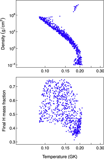
Figure 4. Stellar density vs. temperature (top) and final hydrogen mass fraction vs. temperature (bottom) for sets of (T, ρ,  ) values that reproduce measured elemental abundances in NGC 2419. The results are obtained by random sampling of these three parameters using
  reaction network samples.
Download figure:
Standard image High-resolution imageFor the dilution factors that simultaneosuly reproduce the most extreme measured abundances (on the right-hand side in each panel of Figure 2), we find a range of f = 0.01–0.04. In other words, we do not observe purely processed matter in the stars with the most extreme abundances, although the admixture of pristine matter is very small, consistent with expectation (Section 2.7). This constraint results exclusively from the Mg–K anticorrelation (first panel in Figure 2).
The acceptable values of the final hydrogen mass fraction (bottom panel of Figure 4) scatter over a wide range, i.e., 0.315 ≤  ≤ 0.749. For all solutions shown in Figure 4, except those at very high densities (ρ ≳ 107 g cm−3), the consumed hydrogen mass fraction equals the produced helium mass fraction. We will return to this point in Section 5.1, when comparing our simulated helium abundances with recent observations.
The temperature–density correlation shown in the top panel of Figure 4 is interesting. At any given density, simulated and measured abundances can only be matched for a narrow temperature range. The discontinuity at high densities, ρ ≈ 108 g cm−3, originates from the onset of electron captures on protons. Outside the region occupied by the blue circles, on the low-T and low-ρ side, too little potassium and too much silicon is produced in the simulations, while silicon is underproduced and calcium is overproduced on the high-T and high-ρ side. In the next section, we will relax our assumptions regarding the initial composition and the nuclear interaction rates.
3.3. Monte Carlo Sampling: Initial Composition and Thermonuclear Reaction Rates
The initial mass fractions, Xi, of the elements Li, Be, B, N, F, Ne, P, S, Cl, and Ar are not constrained by observations in NGC 2419. So far we adopted for these elements the abundances predicted by a Galactic chemical evolution model that fits abundances of field stars with the same metallicity as NGC 2419 (Section 2.6 and Table 1). We cannot be certain that our starting abundances correctly predict the initial composition of the polluters. Similarly, we used thus far our best guess for the nuclear interaction rates (i.e., the rates of thermonuclear reactions and weak interactions) provided by STARLIB. But the nuclear rates have uncertainties, derived either from experimental nuclear physics input or from theoretical models (Section 2.4).
For these reasons, we repeated the above Monte Carlo procedure for the parameters T, ρ, and  , but included the initial composition and the nuclear rates in the random sampling. The statistical methods for sampling nuclear interaction rates have been presented recently in the review by Iliadis et al. (2015), and the discussion is not repeated here. It suffices to mention that we adopted a log-normal distribution for both the nuclear rates and the initial abundances, according to

where the log-normal parameters μ and σ determine the location and the width, respectively, of the distribution. For a log-normal probability density, samples, i, of a nuclear rate or an initial abundance, y, are computed from

where ymed and f.u. are the median value and the factor uncertainty, respectively. The quantity pi is a random variable that is normally distributed, i.e., according to a Gaussian distribution with an expectation value of zero and a standard deviation of unity.
For the nuclear rates, both the median value and the factor uncertainty are provided by STARLIB. We emphasize that the factor uncertainty of experimental Monte Carlo reaction rates depends explicitly on temperature. More information on the adopted uncertainties of nuclear rate factors is given in Section 2.4. For the initial abundances of Li, Be, B, N, F, Ne, P, S, Cl, and Ar, we assumed a factor uncertainty of f.u. = 2.5 in the absence of more information. All nuclear rates and initial abundances were sampled independently.
The results of the simultaneous random sampling procedure (for T, ρ,  , all nuclear reaction rates in the network, and initial composition) are displayed in Figure 5. In total, 105 reaction network samples were computed. The significant increase in the scatter of the acceptable solutions (blue circles), compared to Figure 4, is evident. A detailed analysis of which variations in nuclear reaction rate and initial abundance have the largest impact on the scatter is beyond the scope of the present work and will be presented in a forthcoming publication. Test calculations showed, for example, that the sampling of the initial 20Ne and 36Ar abundances contributes significantly to the observed scatter.
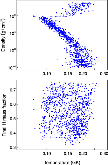
Figure 5. Stellar density vs. temperature (top) and final hydrogen mass fraction vs. temperature (bottom) for sets of (T, ρ,  ) values that reproduce measured elemental abundances in NGC 2419. The results are obtained by random sampling of T, ρ,
  , all nuclear rates in the reaction network, and initial abundances using 105 network samples.
Download figure:
Standard image High-resolution imageThe temperature and density combinations that provide an acceptable match between simulated and measured abundances are not as well confined in parameter space compared to Figure 4, but the results of the simultaneous random sampling procedure display similar features and provide important constraints. The simulated abundances of Mg, Si, K, Ca, Sc, Ti, and V simultaneously match the observations for a temperature range of 78 MK ≤ T ≤ 259 MK (blue circles). Our third main result is that, even if we take the uncertainties in nuclear rates and initial composition into account, we again find a correlation between stellar temperature and density values that provide a satisfactory match between simulated and measured elemental abundances in NGC 2419.
4. POLLUTER CANDIDATES
Polluter candidates must fulfill a number of necessary conditions. First, their temperatures and densities must give rise to the measured abundance pattern, preferably of all relevant elements. Second, their total ejected matter must account for the observed mass budget. Third, their ejecta must be retained by the globular cluster. In this work, we will focus on the first condition and leave an investigation of the latter conditions, apart from a few general comments, to future work.
We show in Figure 6 a magnified section of the top panel of Figure 5, but add hydrogen-burning temperature–density tracks (solid black lines) for several polluter candidates. For two main reasons, we do not expect a potential candidate site to exactly reproduce the T−ρ conditions predicted here. First, the temperature and density, assumed to be constant in our simple model, both vary in realistic hydrogen-burning environments. However, these variations are expected to be relatively small during quiescent burning stages. Second, the temperatures predicted here are directly comparable only to radiative, narrow burning regions. For convective regions, on the other hand, the hydrogen fuel burns in a wide zone at an effective temperature, with most of the nucleosynthesis occurring in the hottest zone. However, the difference between the actual temperature in the hottest zone and the effective temperature for the entire region is relatively small (see Prantzos et al. 2007). In the following, we will adopt our acceptable temperature and density solutions at face value and ask which hydrogen-burning environments are able to produce the appropriate conditions.

Figure 6. Same as the top panel of Figure 5, but with hydrogen-burning T−ρ conditions for several hydrogen-burning polluter candidates superimposed (black solid lines): (i) center of convective hydrogen-burning cores of 15 M⊙ and 120 M⊙ stars ("MS core"; from M. Limongi & A. Chieffi 2015, private communication); (ii) base of radiative hydrogen-burning shell, from the beginning to the tip of the red giant branch, for a 1 M⊙ model ("H shell"; from Karakas 2010); (iii) hot-bottom burning, occurring at the base of the convective hydrogen envelope, during the interpulse period in a 6 M⊙ thermally pulsing AGB star ("AGB"; from Karakas 2010); (iv) hot-bottom burning during the interpulse period in an 8 M⊙ thermally pulsing super-asymptotic giant branch star ("SAGB"; from Doherty et al. 2015); (v) hottest hydrogen-burning zone in classical nova ("CN") models, involving an underlying carbon–oxygen (CO) or oxygen–neon (ONe) white dwarf (from J. José 2015, private communication). The number after the abbreviation stands for the mass of the stellar model assumed. The metallicities of all models, except for classical novae (see text), are similar to the measured value in NGC 2419 (see Section 2.6).
Download figure:
Standard image High-resolution image4.1. Massive Stars
The two tracks shown in Figure 6 labeled "MS core 15" and "MS core 120" refer to hydrogen burning in the convective cores of 15 M⊙ and 120 M⊙ stars, respectively, and were adopted from the latest models of M. Limongi & A. Chieffi (2015, private communication). The assumed metallicity is [Fe/H] = −2.0, which is close to the measured value for NGC 2419 (Section 2.6), and the initial rotational speed amounts to 300 km s−1. Both tracks start at the zero-age main sequence and end when the central hydrogen density has fallen to XH = 0.01. The maximum temperatures achieved in the 15 M⊙ and 120 M⊙ models are 62 MK and 78 MK, respectively. The central density at this stage is 24 g cm−3 and 8 g cm−3, respectively. The T−ρ values of these models come nowhere near the range of acceptable conditions (blue circles in Figure 6). The same conclusion holds for hydrogen burning in the cores of supermassive stars (with M ≈ 104 M⊙). Therefore, the abundance anomalies observed in NGC 2419 cannot be produced by any of the scenarios involving hydrogen burning in the cores of massive stars that have been considered in the literature, including rapidly rotating massive stars (Decressin et al. 2007), massive stars in interacting binary systems (de Mink et al. 2009), or supermassive stars (Denissenkov & Hartwick 2014).
After hydrogen exhaustion in the core, hydrogen continues to burn in a shell until the burning is turned off by the advancing He-burning shell. The physical conditions of the hydrogen-burning shell are mainly driven by the underlying core mass. The 15 M⊙ and 120 M⊙ models referred to above achieve maximum hydrogen shell temperatures of 84 MK and 110 MK, respectively. The corresponding densities are 68 g cm−3 and 22 g cm−3, respectively. Again, these conditions (not shown in Figure 6) are insufficient to account for the measured abundance anomalies in NGC 2419.
4.2. Low-mass Stars
The hydrogen cores of low-mass stars reach insufficient temperatures to make these sites viable polluter candidates. For example, the maximum central hydrogen-burning temperature is <30 MK and <50 MK for a 1.0 M⊙ and a 6.0 M⊙ model, respectively (not shown in Figure 6). However, low-mass stars achieve higher temperatures in the hydrogen-burning shell. The track labeled "H shell 1.0," adopted from (Karakas 2010), represents the T−ρ conditions for a 1.0 M⊙ model, with a metallicity of [Fe/H] = −2.2, at the base of the radiative hydrogen-burning shell, from the beginning to the tip of the red giant branch. The maximum temperature achieved at the end of this track is 57 MK, when the density amounts to 172 g cm−3. These values are far smaller than the conditions indicated by the blue circles in Figure 6. This means that the (second-generation) low-mass stars measured by Mucciarelli et al. (2012) and Cohen & Kirby (2012) in NGC 2419, all located near the tip of the red giant branch, certainly cannot have produced in situ the observed abundance anomalies (Section 1). It also means that hydrogen shell burning in first-generation polluter stars cannot account for the reported abundance anomalies.
4.3. AGB Stars and Super-AGB Stars
AGB stars are the evolved descendents of low- and intermediate-mass stars, with masses in the range of ≈0.8–7 M⊙, depending on metallicity. They consist of a carbon–oxygen core, surrounded by a helium- and a hydrogen-burning shell, and undergo a series of thermal pulses. The highest hydrogen-burning temperatures, and thus the most efficient hydrogen-burning nucleosynthesis, in such stars occurs at the bottom of the convective envelope and is referred to as hot-bottom burning. Stars of higher initial mass reach sufficient temperatures to experience carbon burning in a partially degenerate region near the stellar center and eventually form an oxygen–neon core (Ritossa et al. 1996). They also ascend the AGB, where they are known as SAGB stars, undergo a series of thermal pulses, and experience hot-bottom burning. For a recent review see Karakas & Lattanzio (2014).
The track labeled "AGB 6.0," adopted from Karakas (2010), shows conditions at the base of the convective hydrogen envelope during the interpulse period (hot-bottom burning), for a 6.0 M⊙ thermally pulsing asymptotic giant branch star with a metallicity of [Fe/H] = −2.2. The lifetime of this model star is 74 Myr. The maximum temperature achieved is about 100 MK, which is insufficient to reproduce the measured abundance anomalies in NGC 2419. At the densities representative of this track (≈10 g cm−3), the maximum temperature would need to increase significantly, to about 150 MK, in order to come close to the region occupied by the blue circles. This increase is unlikely, even when fine-turning stellar model parameters such as the mass loss rate or the mass of the hydrogen-exhausted core prior to the start of the AGB, which determines the maximum hot-bottom burning temperature. Therefore, intermediate-mass AGB stars are not favorable candidates for the polluter stars.
We also considered an 8.0 M⊙, Z = 10−4 model (Doherty et al. 2015). The track for hot-bottom burning during the interpulse period of the thermally pulsing SAGB phase is labeled "SAGB 8.0" in Figure 6. The lifetime of this model star is 34 Myr. The model achieves a maximum hydrogen-burning temperature of 136 MK at a density of 9 g cm−3. The models of Ventura et al. (2013), which use the Full Spectrum of Turbulence model of convection, reach a slightly higher maximum temperature of 141 MK (assuming 7.5 M⊙ and Z = 3 × 10⁻⁴) compared to the present models that adopt the mixing-length theory. However, to get close to the region occupied by the blue circles, the maximum temperature would need to increase to 150 MK. Models of super-AGB stars are complex and such an increase in temperature may be achieved by adjusting poorly known model parameters, such as the mass loss rate or the prescription of convective mixing. Therefore, we cannot rule out super-AGB stars as candidate polluters at this time. The parameter space of these stellar models needs to be more fully explored in the future, as advocated by Renzini (2013) and others.
4.4. Novae
Classical novae involve a white dwarf of carbon–oxygen (CO) or oxygen–neon (ONe) composition accreting hydrogen-rich matter from a main-sequence partner via Roche lobe overflow. The transferred matter carries angular momentum and forms an accretion disk. Subsequently, matter accumulates on the surface of the white dwarf under degenerate conditions. Once explosive conditions are met, a thermonuclear runaway occurs, leading to a violent expulsion of matter (José et al. 2006; Starrfield et al. 2008).
Most published classical nova models have assumed accretion of matter with solar composition, although some models of very low metallicity (Z ≈ 10−7 to 2 × 10⁻⁶; José et al. 2007) have also been simulated. Since classical nova models accreting matter of a metallicity appropriate for NGC 2419 have not been computed yet, we adopt the models of J. José (2015, private communication) that assume the accretion of solar metallicity matter from a companion star and a mixing fraction (pre-enrichment) of 50% between accreted and underlying white dwarf matter prior to the thermonuclear runaway. Figure 6 displays three tracks, labeled "CN," for only the hottest hydrogen-burning zone during the thermonuclear runaway. Two models involve underlying carbon–oxygen (CO) white dwarfs with masses of 0.8 M⊙ and 1.0 M⊙, and one model an oxygen–neon (ONe) white dwarf with a mass of 1.15 M⊙. It can be seen that during the evolution the tracks for all three models reach the region of the blue circles. Some of the tracks even extend beyond the range of acceptable T−ρ conditions, implying that other zones in these models, which burn hydrogen at lower temperatures and densities, will also eventually reach the region of the blue circles.
For a metallicity of Z ≈ 10−4 appropriate for NGC 2419, white dwarfs with masses of M ≳ 0.8 M⊙ have a progenitor age of ≲0.5 Gyr, i.e., the time between the zero-age main sequence and the point of entering the white dwarf cooling curve (Romero et al. 2015). This leaves sufficient time for novae involving massive white dwarfs to pollute the intracluster medium before the formation of the second-generation stars.11
Classical novae could thus be interesting polluter candidates, as previously proposed by Smith & Kraft (1996). Recent work also suggested novae involving isolated white dwarfs, i.e., white dwarfs that accrete directly from the intracluster medium, as polluters (Maccarone & Zurek 2012). The authors state that a potential problem with their conjecture could be that "... largely speaking, classical novae do not burn beyond chlorine ...." On the contrary, once appropriate hydrogen-burning conditions are established (Figure 6), potassium, for example, will be produced from pre-existing argon, as explained in Section 2.5.
Novae have so far received little attention in the literature as polluter candidates. Recent work reported a present frequency of 0.05 novae per year per globular cluster (Henze et al. 2013), a value that is much higher than previous estimates for the nova rate in globular clusters. The predicted upper limit for the ejected mass per nova is (2–3) × 10−3 M⊙ (Shara et al. 2010). If we assume 0.5 Gyr for the time period over which novae polluted the intracluster medium before the formation of the second-generation stars (Section 2.1) and a 10% efficiency for converting nova ejecta into new stars, we find ≈0.05 yr−1 × 0.5 × 109 yr × 0.1 × 10−3 M⊙ = 2.5 × 10³ M⊙ for the total mass in the cluster that could be processed by novae. On the other hand, NGC 2419 has a mass of 9 × 10⁵M⊙ (Section 1) and about 30% of the stars in this cluster are potassium-enriched (Cohen & Kirby 2012; Mucciarelli et al. 2012), with small dilution factors of f ≤ 0.04 (i.e., most of the enriched matter consists of processed rather than pristine material; see Section 3.2). Therefore, the polluters ejected a total mass of ≈9 × 10⁵ M⊙ × 0.3 = 2.7 × 10⁵ M⊙, about two orders of magnitude higher than what we expect from novae. However, some of the above parameters are highly uncertain. For example, the past nova rate was perhaps much higher, especially if the white dwarfs accreted directly from the dense intracluster medium in the early globular cluster (Maccarone & Zurek 2012). The question whether or not novae can quantitatively account for the reported abundance anomalies has to await new detailed models of white dwarfs accreting matter of a composition consistent with NGC 2419, either from a main-sequence companion or directly from the intracluster medium.
5. ADDITIONAL CONSTRAINTS FROM OBSERVED He AND C, AND FROM FUTURE MEASUREMENTS
5.1. Helium
Photometry of NGC 2419 provides evidence for a spread in the initial helium abundance of the cluster stars. Lee et al. (2013) inferred that the red giant branch is split into two distinct subpopulations, with 70% of the stars showing a primordial helium abundance and the other 30% showing helium mass fractions near 0.42, corresponding to an enhancement of ΔY ≈ 0.19. Furthermore, Di Criscienzo et al. (2015) inferred three distinct populations from the photometry of the horizontal branch: (i) one with an initial helium abundance close to primordial (Y = 0.25), (ii) a small population with an intermediate helium abundance of 0.26 < Y ≲ 0.29, and (iii) a large population with a high initial helium abundance of Y ≈ 0.36, which is derived from the extreme blue horizonal branch.
Di Criscienzo et al. (2015) state that "...the initial helium abundance of this extreme population is in nice agreement with the predicted helium abundance in the ejecta of massive AGB stars of the same metallicity as NGC 2419. This result further supports the hypothesis that second-generation stars in GCs [globular clusters] formed from the ashes of intermediate-mass AGB stars...." In massive AGB stars and super-AGB stars, most of the surface helium originates from the second dredge-up, with only a minor contribution from hot-bottom burning. In our constant T−ρ model, on the other hand, potassium and helium are concurrently produced during high-temperature hydrogen burning. In Figure 7, we show the same results as in Figure 5 (top) and in Figure 6, but now different colors indicate the final helium mass fraction resulting from our simulations. The red circles indicate final helium mass fractions of 0.30 ≤  ≤ 0.45, corresponding to the He-rich populations (Lee et al. 2013; Di Criscienzo et al. 2015), while the green circles label solutions with other values of
  . It can be seen that the elusive polluters that gave rise to the observed Mg–K anticorrelation in NGC 2419 could account simultaneously for the enhanced initial helium abundance (red circles), inferred by Lee et al. (2013) and Di Criscienzo et al. (2015), over the entire density range (ρ = 10−4–1011 g cm−3) explored in the present work. In other words, polluter candidates other than AGB or super-AGB stars are also able to account for the helium measurements, assuming that K and He are produced during the same high-temperature hydrogen burning process. If this was indeed the case, then the helium measurements further constrain the hydrogen-burning temperature range of the polluters, as indicated by the reduced scatter of the red circles compared to the green circles in Figure 7.
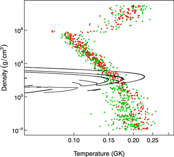
Figure 7. Stellar density vs. temperature for sets of (T, ρ,  ) values that reproduce measured elemental abundances in NGC 2419. The circles and the T−ρ tracks are the same as those shown in Figure 5 (top) and Figure 6, respectively. Colors indicate ranges of the final helium mass fraction resulting from our simulations: 0.30 ≤
  ≤ 0.45 (red) and
  > 0.45 or
  < 0.30 (green). The red circles correspond to T−ρ conditions that yield a helium abundance consistent with the recent analysis of extreme populations in NGC 2419 (Lee et al. 2013; Di Criscienzo et al. 2015).
Download figure:
Standard image High-resolution image5.2. Lithium
Our simulated lithium abundance depends strongly on the T−ρ conditions assumed for hydrogen burning, and therefore lithium measurements would further constrain the parameter space of the polluters. Unfortunately, lithium has not been observed in NGC 2419. According to Cohen & Kirby (2012), "...the lithium line at 6707 Å cannot be detected in the summed spectra of either group of NGC 2419 giants...." Presumably these giant stars have depleted their lithium in the usual way.
We note that some globular clusters, e.g., NGC 1904 and NGC 2808 (D'Orazi et al. 2015), show a reduced Li content in the proposed second-generation stars, with high Na and low O. This is what would be expected from hydrogen burning in the polluters, because Li is destroyed at temperatures as low as 2 MK. However, there are other globular clusters, e.g., NGC 6397 (Lind et al. 2009), M4 (D'Orazi & Marino 2010; Mucciarelli et al. 2011), M12 (D'Orazi et al. 2014), and NGC 362 (D'Orazi et al. 2015), where both generations of stars show essentially the same Li content, which requires that the polluters must also produce Li. This is one reason for the continued investigation of AGB and super-AGB stars as the polluters. However, it is interesting to note that classical novae, implicated by our results, can also produce Li. Of course, both proposed polluter scenarios have quantitative problems in producing the required amount of Li.
5.3. Carbon, Nitrogen, Oxygen
Consider again Figure 2, showing in each panel on the right-hand side the extreme observed stars, consisting of matter that underwent an elusive hydrogen-burning process during a previous stellar generation. These extreme stars were likely born with a different He and CNO composition compared to normal stars (located on the left-hand side in each panel of Figure 2) that were presumably born with a composition similar to field stars of the same metallicity (see Table 1).
Figure 8 (top) shows our simulated final abundances of the light nuclides 1H, 4He,12C, 13C, 14N, 15N, 16O, 17O, and 18O in processed matter. The results are obtained from the same Monte Carlo simulation shown in Figure 5 (blue circles) and include the random sampling of nuclear reaction rates and initial composition. The bottom panel displays the final carbon isotopic ratio. At very low densities (ρ ≲ 10 g cm−3), the simulations predict a steadily rising carbon isotopic ratio for decreasing density. At densities above ρ ≈ 102 g cm−3, nitrogen is by far the most abundant CNO isotope and the carbon isotopic ratio is 12C/13C ≈ 0.1.
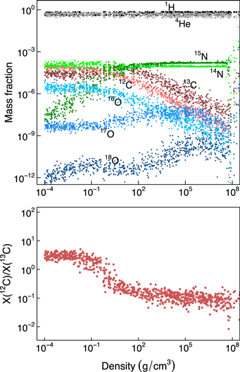
Figure 8. Simulated final abundances of 1H, 4He,12C, 13C, 14N, 15N, 16O, 17O, and 18O (top panel) and ratio of carbon isotopic mass fractions (bottom panel) in processed matter vs. stellar density. The results are obtained from the same Monte Carlo simulation shown in Figure 5 (blue circles) and include the random sampling of nuclear reaction rates and initial composition.
Download figure:
Standard image High-resolution imageIt would be interesting to compute a number of stellar evolutionary models of low-mass stars, with initial compositions chosen from Figure 8, and to track the changes in the CNO abundances and in the 12C/13C ratio during the evolution of a low-mass star to the tip of the red giant branch. The large changes in the initial 4He and CNO abundances, compared to canonical models, will have a strong effect in terms of how fast the stars evolve and their location in the color–magnitude diagram; in particular, the helium enrichment will cause the stars to appear hotter and bluer. Therefore, it may be possible to further constrain the T−ρ conditions of the polluters by comparing, for the extreme stars, the measured and the simulated luminosity and elemental carbon abundance. Future measurements of the 12C/13C isotopic ratio could also be important in this regard. This reasoning explicitly assumes that in the polluters the CNO isotopes underwent the same high-temperature hydrogen burning process as the heavier elements (Mg to V), and no additional, non-hydrogen, burning process. We will leave this investigation to future work.
5.4. Oxygen versus Sodium
All Galactic globular clusters that have been examined for the O–Na correlation have (so far) shown this signature (see Figure 2 in Gratton et al. 2012). But as pointed out in Section 2.3, sodium and oxygen have been measured simultaneously in NGC 2419 for only three red giants (Cohen & Kirby 2012). The available data, shown in Figure 9, are not sufficient to establish a relationship between the abundances of these two elements. The solid line shows the results of a simulation with T = 160 MK, ρ = 900 g cm−3, and  = 0.70, i.e., the same conditions referred to in Figure 2. The crosses, from left to right, correspond to dilution factors of f = 0.02 (mostly processed matter) to f = 1000 (pristine matter). Very similar results are obtained for all T−ρ conditions shown as blue circles in Figure 4, except at very high densities of ρ > 5 × 10⁷ g cm−3.
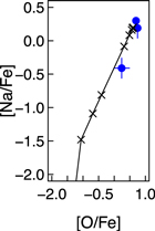
Figure 9. Sodium vs. oxygen abundance for red giants in NGC 2419 (data from Cohen & Kirby 2012). Simulations are shown in black for the conditions T = 160 MK, ρ = 900 g cm−3, and  = 0.70: the solid line is obtained by mixing one part of processed matter with f parts of pristine matter; the first cross on the left correspond to a dilution factor of f = 0.02 (mainly processed matter), and the last cross on the right to f = 1000 (pristine matter). Notice that the simulations predict an O–Na correlation instead of an anticorrelation.
Download figure:
Standard image High-resolution imageIf oxygen and sodium underwent the same high-temperature hydrogen burning process as the heavier elements (Mg to V), and no additional burning process, then our calculations predict an O–Na correlation. On the other hand, if instead an O–Na anticorrelation is observed, then low-temperature and high-temperature hydrogen burning operated independently in NGC 2419, perhaps in different first-generation stars or at different locations in the same stars (Section 2.3). Future measurements are highly desirable, although the observation of oxygen lines in the cool and metal-poor giants of NGC 2419 will be very challenging.
6. SUMMARY
We reported here on the first comprehensive investigation of the parameter space involving temperature, density, consumed hydrogen abundance, thermonuclear reaction rates, and initial chemical composition, to constrain the list of candidate sites that produced the recently measured abundance anomalies in the globular cluster NGC 2419. The observed abundances of magnesium, silicon, and scandium are correlated with potassium, while the abundances of calcium, vanadium, and titanium are nearly constant. These signatures provide important clues regarding their origin.
We assumed a model with constant temperature and density and allowed for mixing (dilution) between nuclearly processed and pristine matter. We investigated under which conditions all of the measured abundances of elements up to vanadium can be reproduced, assuming the full range of dilution factors. Using a reaction network Monte Carlo method, we randomly sampled the stellar temperature, stellar density, and the consumed hydrogen mass fraction to find conditions that can account for the observations. Variations of thermonuclear reaction rates and initial composition were included in the random sampling. We find a correlation between stellar temperature and density values that provide a satisfactory match between simulated and observed elemental abundances of Mg, Si, K, Ca, Sc, Ti, and V in NGC 2419. Except at the highest densities (ρ ≳ 108 g cm−3), the acceptable conditions range from ≈100 MK at ≈108 g cm−3 to ≈200 MK at ≈10−4 g cm−3.
We reviewed hydrogen-burning sites from a nucleosynthesis point of view and find that low-mass stars, AGB stars, massive stars, and supermassive stars are unlikely to account for the measured abundance anomalies in NGC 2419. Super-AGB stars could be viable candidates for the polluter stars if stellar model parameters can be fine-tuned to produce higher temperatures. Novae, involving either CO or ONe white dwarfs, could be interesting polluter candidates, but a current lack of low-metallicity nova models precludes firmer conclusions. Apart from considerations of nucleosynthesis, all polluter candidates that have been suggested previously (massive stars, AGB stars, super-AGB stars, interacting binaries, novae, or supermassive stars) have a mass budget problem (see discussion in Bastian et al. 2015).
The polluter candidates discussed above and in the literature cover a relevant density range of 10 g cm−3 ≲ ρ ≲ 104 g cm−3 (see Figure 6). As already pointed out, we also find acceptable solutions for matching calculated and measured abundances in NGC 2419 for much higher (ρ = 104–1011 g cm−3) and for much lower (ρ = 10−4–10 g cm−3) densities, with temperatures in the range of 80 MK ≲ T ≲ 260 MK. It is not clear at this time which astrophysical environments could give rise to such conditions.
Finally, we discussed the possibility of obtaining additional T−ρ constraints for the (first-generation) polluters by evolving (second-generation) stars with non-canonical initial abundances and by comparing, for the extreme stars in NGC 2419, the model results for the luminosity and elemental carbon abundance to the observations. We also pointed out the importance of new O and Na abundance measurements. If oxygen and sodium underwent the same high-temperature hydrogen burning process as the heavier elements (Mg to V), and no additional burning process, then our simulatuions predict an O–Na correlation instead of an anticorrelation for NGC 2419. If instead an O–Na anticorrelation is observed in the future, then low-temperature and high-temperature hydrogen burning operated independently in NGC 2419, either in different first-generation stars or at different locations in the same stars.
We would like to thank Jordi José, Marco Limongi, and Alessandro Chieffi for providing up-to-date temperature–density tracks. Helpful comments from Lori Downen, Bart Dunlap, Alex Heger, Fabian Heitsch, Sean Hunt, Richard Longland, Sumner Starrfield, Chris Tout, and David Yong are highly appreciated. A.I.K. is grateful for the support of the NCI National Facility at the ANU, and was supported through an Australian Research Council Future Fellowship (FT110100475). This work was supported in part by the U.S. Department of Energy under Contract No. DE-FG02-97ER41041, and under Australian Research Councils Discovery Projects funding scheme (project number DP120101815). C.I. was partially supported by the MoCA Distinguished Visitor Program at Monash University.
Footnotes
- 7
A small fraction of field stars exhibit abundance anomalies characteristic of some globular cluster stars. These field stars are believed to have escaped during the dynamical history of their parent globular cluster (see Lind et al. 2015, and references therein).
- 8
For a different interpretation that does not involve multiple stellar generations, see Bastian et al. (2013).
- 9
According to common convention, abundances are given as
![${[A/B]}_{\star }\equiv {\mathrm{log}}_{10}{({N}_{A}/{N}_{B})}_{\star }-{\mathrm{log}}_{10}{({N}_{A}/{N}_{B})}_{\odot }$](/img/lazy-loading-placeholder.gif) , where Ni are number abundances of elements A and B observed in a star (⋆) or the Sun (⊙); while the quantity is unitless, differences between two values are expressed in units of dex ("decimal exponent").
, where Ni are number abundances of elements A and B observed in a star (⋆) or the Sun (⊙); while the quantity is unitless, differences between two values are expressed in units of dex ("decimal exponent"). - 10
Available at: http://starlib.physics.unc.edu/index.html.
- 11
Let us consider a specific example. For a metallicity of Z = 10−4, a star with an initial mass of 7 M⊙ will become a 1.2 M⊙ white dwarf of O–Ne composition in about 44 Myr (Doherty et al. 2015). The white dwarf needs some time to cool before a nova outburst can take place; if the white dwarf is initially too luminous, the envelope is not highly degenerate when the thermonuclear runaway develops and only a mild thermonuclear runaway with no mass ejection may occur. Nova simulations have obtained mass ejection for luminosities as high as
= 0.1 (Starrfield et al. 1985), 0.3 (Yaron et al. 2005), and 1.0 (Hernanz & José 2008). According to García-Berro et al. (1997), it takes only 61 Myr for the 1.2 M⊙ white dwarf of O–Ne composition to cool to a luminosity of = 0.1. Therefore, the entire evolution from the zero-age main sequence to the point where mass accretion onto the white dwarf can produce a nova outburst takes about 100 Myr.
![${[A/B]}_{\star }\equiv {\mathrm{log}}_{10}{({N}_{A}/{N}_{B})}_{\star }-{\mathrm{log}}_{10}{({N}_{A}/{N}_{B})}_{\odot }$](https://content.cld.iop.org/journals/0004-637X/818/1/98/revision1/apj522459ieqn1.gif)
![$[A/B]$](https://content.cld.iop.org/journals/0004-637X/818/1/98/revision1/apj522459ieqn2.gif)

