


ABSTRACT
We study the umbral waves as observed by chromospheric imaging observations of two sunspots with the New Solar Telescope at the Big Bear Solar Observatory. We find that the wavefronts (WFs) rotate clockwise and form a one-armed spiral structure in the first sunspot, whereas two- and three-armed structures arise in the second sunspot where the WFs rotate anticlockwise and clockwise alternately. All the spiral arms display propagation outwards and become running penumbral waves once they cross the umbral boundaries, suggesting that the umbral and penumbral waves propagate along the same inclined field lines. We propose that the one-armed spiral structure may be produced by the WF reflections at the chromospheric umbral light bridge, and the multi-armed spirals may be related to the twist of the magnetic field in the umbra. Additionally, the time lag of the umbral oscillations in between the data of He i 10830 Å and  Å is ∼17 s, and it is ∼60 s for that in between the data of 304 Å and
  Å. This indicates that these disturbances are slow magnetoacoustic waves in nature, and that they propagate upward along the inclined lines with fast radial expansions causing horizontal velocities of the running waves.
Export citation and abstract BibTeX RIS
1. INTRODUCTION
Intensity and velocity observations in various spectral lines have revealed the existence of 5/3 minute oscillations (see review by Thomas 1985; Lites 1992; Staude 1999; Bogdan & Judge 2006 and references therein) in the umbral photosphere (Bhatnagar & Tanaka 1972)/chromosphere (Beckers & Schultz 1972; Giovanelli 1972). The 5 minute oscillations are predominantly a photospheric phenomenon. Their amplitude decreases with increasing height and they can hardly be detected in the upper chromosphere and transition region. On the other hand, the oscillatory power in the 3 minute band shows a dominant peak in the sunspot chromosphere (e.g., Lites 1986; Yoon et al. 1995) and in the transition region between the chromosphere and the corona (Gurman et al. 1982). A manifestation of chromospheric umbral oscillations is umbral flashes (UFs), which were first discovered by Beckers & Tallant (1969) in Ca ii H and K filtergrams and spectrograms of a sunspot. UFs appear in the form of narrow bright lanes stretched along the light bridges (LBs) and around clusters of umbral bright points (Yurchyshyn et al. 2015) when the velocity amplitudes exceed a threshold, e.g., 5 km s−1 for the Ca ii K line. UFs are rarely observed in Hα and perhaps only when the velocity amplitude is large enough (e.g., Tziotziou et al. 2007).
In this paper, we concentrate on the chromospheric umbral oscillations and the running waves associated with them. There are several theoretical models for the nature of the 3 minute umbral oscillations. Scheuer & Thomas (1981) and Thomas & Scheuer (1982) proposed that the oscillations are driven by a resonance of fast magnetoacoustic waves, located in the photosphere and subphotospheric layers, that are excited by overstable convection (a photospheric resonator). Many subsequent studies of umbral oscillations tried to find the eigenmodes of sunspot oscillations related to the photospheric resonator under closed boundary conditions (Hasan 1991; Hasan & Christensen-Dalsgaard 1992; Banerjee et al. 1995, 1997, 2002; Gore 1997, 1998; Wood 1997) or open ones (Cally & Bogdan 1993; Cally et al. 1994; Bogdan & Cally 1997; Lites et al. 1998) of one atmosphere permeated by a uniform magnetic field aligned with the constant gravitational acceleration. Eigenmodes with periods from several tens of minutes (g-modes) to several tens of seconds (p-modes) have been found (Zhukov 2002). Another model, originally proposed by Zhugzhda & Locans (1981) and recently improved by Zhugzhda & Sych (2014), involves the resonant trapping of slow-mode waves within a cavity located in the chromospheric umbra (a chromospheric resonator). In addition, some efforts have been made toward reconciling photospheric and chromospheric resonators (Lee & Yun 1987; Zhugzhda & Sych 2014) and the oscillation eigenmodes and atmospheric wave filtering (Zhukov 2005).
Running penumbral waves in velocity and intensity observations were first reported by Giovanelli (1972) and Zirin & Stein (1972). Later, they were found in the photosphere as well (Musman et al. 1976), but there they appear to be more intermittent and to have higher radial phase velocity (40–90 km s−1) than the waves in Hα. Whereas the velocity amplitudes are less in the photosphere than in the chromosphere, the density is very low there and most of the wave energy lies in the photosphere and subphotosphere. Larger amplitudes on the disk-side penumbra demonstrate an alignment of the oscillations along the magnetic field. Running waves are also detected in the umbra, but the waves were believed to be unrelated to those in the penumbra (Kobanov & Makarchik 2004). In the chromosphere, the frequency of travelling waves decreases as they propagate from the umbra into the outer penumbra (e.g., Lites 1988). A similar effect is also found in measurements of the propagation velocity of travelling waves (Brisken & Zirin 1997; Sigwarth & Mattig 1997; Alissandrakis et al. 1998; Kobanov & Makarchik 2004; Tziotziou et al. 2006, 2007). Generally, the waves decelerate from 40 km s−1 near the inner part of the penumbra to 10 km s−1 or less near the outer edge of the penumbra. More recently, from a multi-wavelength study including the coronal channels of the Atmospheric Imaging Assembly (AIA) on board the Solar Dynamics Observatory (SDO), Jess et al. (2015) revealed the presence of a wide range of frequencies, with longer periodicities preferentially occurring at increasing distance from the umbra. The phase speeds also tend to decrease with increasing periodicity as the waves propagate away from the umbral barycenter. These observations also suggest that these slow waves are driven by a regular coherent source. The physical nature of running penumbral waves has been controversial. Some researchers have regarded them as trans-sunspot waves originating from umbral oscillations since they detected waves starting from the umbra and propagating through the penumbra (e.g., Alissandrakis et al. 1992; Tsiropoula et al. 1996, 2000). However, others suggest that the trans-sunspot (i.e., outward) motion is apparent to a given line of sight, and that these oscillations actually represent the upward propagation of field-guided magnetoacoustic waves from the photosphere (e.g., Christopoulou et al. 2000, 2001; Georgakilas et al. 2000; Rouppe van der Voort et al. 2003; Bogdan & Judge 2006; Kobanov et al. 2006; Bloomfield et al. 2007; Jess et al. 2013, 2015). The gradual change in the inclination of the penumbral field lines is responsible for changes in the oscillation periods and phase speeds.
The connection between the 3 minute umbral oscillations and running penumbral waves is yet to be fully understood. Lites et al. (1998) observed a continuity of disturbances across the umbra–penumbra boundaries of one sunspot. He proposed that either the penumbral waves in the inter-penumbra are driven by the umbral oscillations or the umbral and penumbral oscillations share a common physical basis. Tsiropoula et al. (1996, 2000), Tziotziou et al. (2002), and Alissandrakis et al. (1992, 1998) provided clear evidence of waves originating from oscillating elements inside the umbra and propagating through the penumbra. However, many authors have also shown that the running penumbral waves are not an extension of the 3 minute umbral waves (e.g., Kobanov & Makarchik 2004; Kobanov et al. 2008). The measured propagation velocity of the umbral waves turned out to be much higher, 40–70 km s−1. Whereas 3 minute umbral oscillations in the chromosphere are not considered as the source of the running penumbral waves (Christopoulou et al. 2000; Kobanov & Makarchik 2004; Bloomfield et al. 2007), researchers realized that the chromospheric oscillations in umbrae (UFs) and the running penumbral waves might be different manifestations of the same phenomenon produced by a common source in the photosphere (Zhugzhda et al. 1984; Christopoulou et al. 2001; Rouppe van der Voort et al. 2003; Bloomfield et al. 2007; Tziotziou et al. 2007). Their differences arise from the transmitted wave power available for propagation along differently inclined field lines. Löhner-Böttcher & Bello González (2015) analyzed the Interferometric BIdimensional Spectropolarimeter (IBIS/DST) data and found signatures of running penumbral waves in photospheric layers. This further supports the scenario of running penumbral waves being upward-propagating slow-mode waves guided by the magnetic field lines.
Recently, Sych & Nakariakov (2014) detected umbral wavefronts (WFs) with an evolving two-armed spiral that rotated anticlockwise, suggesting that the umbral waves propagate not only in the radial direction but also in the polar angle direction. In this work, utilizing the observations of the New Solar Telescope (NST, Cao et al. 2010; Goode & Cao 2012), we find additional propagating patterns of the umbral waves. We expect that the new results reported here could help to clarify some problems of sunspot oscillations, e.g., the source of the 3 minute oscillations and their connections with the running penumbral waves. The remainder of this paper is arranged as follows. Section 2 will discuss the observations of target sunspots and the data reduction methods. Section 3 will explain the main results of the analysis. In Section 4 we further discuss the findings presented in the preceding section. Finally, Section 5 summarizes the findings presented in the work.
2. DATA AND REDUCTION
The NST observations were performed on two main sunspots (see Figure 1) of NOAA active regions 12127 (sunspot 1, located at S09E08 on 2014 August 1) and 12132 (sunspot 2, located at S19E04 on 2014 August 5). The data on sunspot 1 were taken at 17:15 UT–17:55 UT, and the data on sunspot 2 at 18:20 UT–19:20 UT. Chromospheric images were acquired every 23 s by scanning of the Hα spectral line from the blue wing −1 Å to the red wing +1 Å with a step of 0.2 Å. The field of view (FOV) is 70'' with a pixel size of  . Images of the TiO (7057 Å) line are used to identify the boundary between umbra and penumbra as this absorption line forms only at temperatures below 4000 K and it is well suited for observing the umbra. To study the effect of the inclination of magnetic field on the wave period, we used the vector magnetogram of sunspot 1 from the Spectropolarimeter of the Solar Optical Telescope (Kosugi et al. 2007; Tsuneta et al. 2008) on board Hinode, and that of sunspot 2 from the Helioseismic and Magnetic Imager (HMI, Schou et al. 2012) on board the SDO.
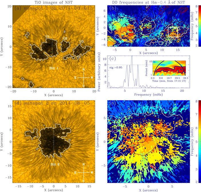
Figure 1. Left panels: TiO images of the sunspots in NOAA 12127 and NOAA 12132 as observed on August 1 and August 5, respectively. Three umbral regions of sunspot 1 are marked as U1, U2, and U3. Two dotted lines mark two virtual slits (1 and 2) for further analysis. Right panels (b) and (e): power maps of the dominant oscillation frequencies in the umbrae of sunspots 1 and 2, respectively. The red contours show the cosines of magnetic field inclinations with levels of 0.85, 0.95, and 0.99. Panel (c) and its inset show the Fourier power spectra and wavelet power corresponding to the averaged  Å intensity signals within the dotted square in panel (b). The white contours on panels outline the umbral boundaries.
Download figure:
Standard image High-resolution imageTo investigate the umbral oscillations in sunspot 2 at different solar altitudes, in addition to the Hα data, we also used images of the narrow band (band-pass: 0.5 Å) of He i 10830 Å of the NST with a pixel size of  and time cadence of 15 s as observed on August 5, and the images of 304 Å taken by the SDO/AIA. These lines allow us to study the umbral oscillations in the chromosphere (Hα line), in the upper chromosphere (He i 10830 Å line), and in the transition and lower corona region (304 Å line). For each sunspot, we used the first image at
  Å as a reference to align all the other images at the same passband. In this procedure, the relative shifts to the first image are kept, and are then used to align the Hα images in the other passbands (all the images observed every 23 s are assumed here to be already co-aligned). Similarly, with the reference image, it is not difficult to co-align it with the images of other instruments.
The  Å images show that there are electric fan-like shadows emerging periodically and they rotate very fast around the umbral centers of the two sunspots. Also, the direction of rotation of the shadows in sunspot 2 can alternate between clockwise and anticlockwise. We attempt to use a phase-speed filter (see the
  km s−1 are used widely in this paper, and the physical reason is given in Section 3.1.
In addition, we calculate the center of gravity of the Hα line profile corresponding to each pixel to estimate the Doppler shift relative to the reference line center obtained by averaging over the whole FOVs of sunspots 1 and 2 in Figure 1 (the blank fields excluded in the figure). The passbands of the line have been expanded from 11 to 110 by interpolation to improve the fitting for better velocity estimates.
3. RESULTS
3.1. Umbral Oscillations and Running Waves
Figure 1 presents TiO images of sunspot 1 (panel (a)) and sunspot 2 (panel (d)). For sunspot 1, we focus only on its right side, on three umbrae marked as U1, U2, and U3. The left umbra is often obscured by some peacock-like jets, so we do not consider it for further analysis. Following Jess et al. (2013), we generate a power spectrum (see technique details in Scargle 1982; Horne & Baliunas 1986; Yuan et al. 2011) corresponding to each spatial pixel for temporal sequences of the Hα −0.4 Å intensity, and then extract the dominant oscillation (DO) frequency. Zero value is assigned at those pixels where the DO frequency is less than the confidence threshold of 0.95. Panels (b) and (e) show the DO frequency distributions (power maps) of Hα −0.4 Å for sunspots 1 and 2, respectively.
A part of U3 (marked by a white square in panel (b)) is selected for further analysis. Corresponding to the averaged signal within this boxed region, the Fourier power spectrum and wavelet phase plots are shown in panel (c) and its inset. It is clear that a frequency of ∼6.8 mHz (2.45 minutes) lasting for about 35 minutes is dominant. The figure also exhibits some secondary frequencies around 5.5, 6.2, and 8.4 mHz. These frequencies are consistent with the theoretical predictions of eigenmodes of photospheric umbral oscillation (Cally & Bogdan 1993; Bogdan & Cally 1997; Zhukov 2005) and/or chromospheric multi-passband filters for the slow waves (Zhugzhda 2008). In addition, the other umbrae (U1, U2, and the umbra in sunspot 2) are found with similar frequency distributions to U3 (not shown).
In panels (b) and (e), cosine contours of field inclinations (deep red contours) are overplotted. Generally, they demonstrate that the DO frequency increases with the cosine of inclination (Madsen et al. 2015). However, some regions are different, for example, in panel (b) around  and
and  (as compared to that around
  and
and  ), the higher-frequency (
 mHz) elements correspond to a smaller cosine of inclination. This may be due to the complex topology and the strong inherent dynamics of sunspot 1. Physical characteristics in such regions have so many peculiarities that we should treat the obtained results with particular caution.
Evaluations of the propagating velocities of umbral and penumbral waves in the two sunspots are displayed in panels (a) and (b) of Figure 2. Time–distance maps corresponding to the two virtual slits crossing the umbrae of sunspots 1 and 2 (see Figure 1) are shown. Umbral and penumbral boundaries are shown by the solid lines at  and
and  in panel (a) and at
  and
and  in panel (b). Although some umbral ridges are branching or merging (Chae et al. 2014) near the boundaries, most ridges of penumbral waves extend from the umbra to the penumbra, which indicates that they originate in the umbra (Alissandrakis et al. 1992, 1998; Tsiropoula et al. 1996, 2000; Lites et al. 1998; Tziotziou et al. 2002).
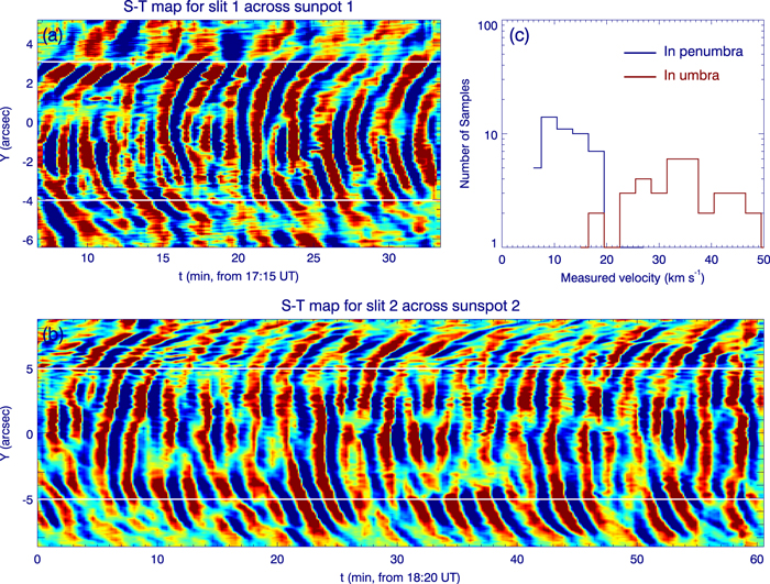
Figure 2. Velocities of the umbral and penumbral waves in sunspots 1 and 2. Panels (a) and (b) are the time–space diagrams corresponding to slits 1 and 2 as marked in Figure 1, respectively. The solid lines mark the umbral and penumbral boundaries. Panel (c) is a histogram of the measured velocities in the umbral (red) and penumbral (blue) regions.
Download figure:
Standard image High-resolution imageCalculating the gradient of the ridges, we obtain the wave velocities as shown in panel (c). The histogram displays that the umbral waves have a velocity distribution from ∼15 to 50 km s−1, and the penumbral waves from 6 to 20 km s−1 with a peak at ∼10 km s−1. Based on the distributions, we somewhat arbitrarily choose v = 14 km s−1 to distinguish between umbral and penumbral waves, and v = 4 km s−1 to distinguish between them and lower-speed waves.
3.2. One-armed Spiral Structures in Sunspot 1
In Figure 3 we study the evolution of the spiral structure as seen within sunspot 1. It shows that at 17:49:06 UT, a dark ribbon-like WF emerges at the north-east umbral boundary (the red dotted contours). It moves subsequently in both radial (see black arrows) and clockwise azimuthal (see white arrows) directions. The radial and azimuthal velocities are  km s−1 at 17:51:00 UT (panel (f)) and
  km s−1 at 17:50:14 UT (panel (d)), respectively. Specifically, for vr we measure the radial distance between the two arc ribbons at 17:49:29 UT and 17:51:00 UT (the WF shown by black arrows). For va we measure the azimuthal distance between the two black ribbons at 17:49:52 UT and 17:50:14 UT (the WF shown by white arrows). The errors come from the diffused WF profiles. At 17:51:22 UT (panel (g)), a one-armed spiral structure is formed. At 17:51:45 UT, the next dark ribbon arises at the north-east umbral boundary again, suggesting that the previous period of umbral oscillation ended (with
  minutes).
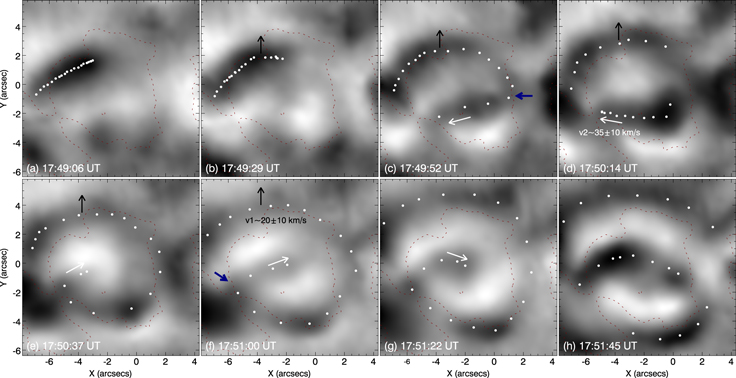
Figure 3. Formation of the one-armed spiral structure of one WF in U1 of sunspot 1 (seen in the phase-velocity filtering images of  Å with
  km s−1. The white solid circles highlight the propagating trajectory of the WF and the red dotted lines outline the umbral boundary. The black and white arrows indicate the directions of propagation of the wave, and the blue arrows mark locations where the wave is reflected. Note that the bright patch in the top-left umbral boundary region of panel (f) is caused by the dark WF in panel (b) radially expanding out of the region. However, the contrary is the case for the central region in panels (h) and (e), where the WF just reaches here and then the region gets dark.
Download figure:
Standard image High-resolution image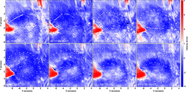
Figure 4. Similar to Figure 3, but for the same WF seen in the images of Hα Doppler velocity.
Download figure:
Standard image High-resolution imageThe one-armed spiral structures are also found in umbrae U2 (Figure 5) and U3 (Figure 6), which show radially expanding and clockwise rotation as well. The timescale for formation of the spiral structure is about 2.6 minutes in U2 and 2.3 minutes in U3. The typical radial and azimuthal velocities are  and
and  km s−1 in U2, and
  and
and  km s−1 in U3. These timescales and velocities are of the same order as those in U1.
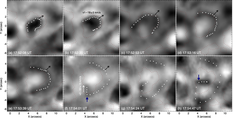
Figure 5. Similar to Figure 3, but in U2.
Download figure:
Standard image High-resolution image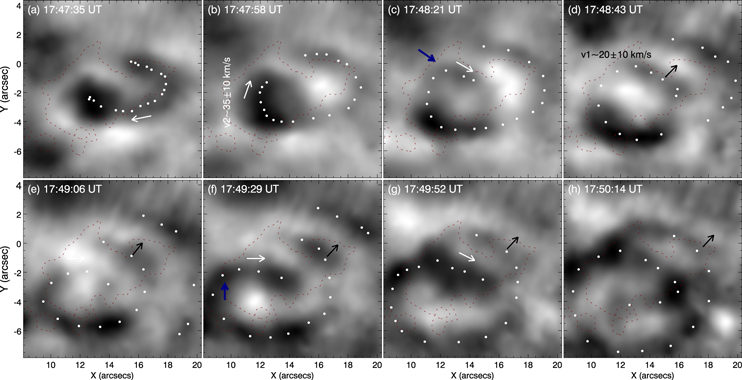
Figure 6. Similar to Figure 3, but in U3.
Download figure:
Standard image High-resolution imageHow do the propagating WFs develop into such a one-armed spiral pattern? We find that they would change their azimuthal directions of propagation abruptly at some locations (see the blue arrows at 17:49:52 UT and 17:51:00 UT in U1, 17:54:01 UT and 17:54:47 UT in U2, and 17:48:21 UT, 17:49:29 UT, and 17:50:14 UT in U3). It appears that the WFs are reflected at the above locations. We also find these locations of reflection near the photospheric umbral boundaries (marked by blue arrows in Figures 3, 5, and 6), which might be acting as natural barriers to partially prevent WFs escaping from the umbrae.
However, we are aware that the given boundary refers to the deep photosphere while the studied oscillations refer to the chromosphere (the height difference is 1500–2000 km). Moreover, according to general views, in the chromosphere, waves propagate along magnetic field lines. Thus, we attempt to check Doppler velocity in the Hα spectral line to find out more information about the direction of propagation of umbral waves. Figure 4 shows such maps of Doppler velocity in U1. As compared to Figure 3, the WF seen in them is more diffused with a bias toward blueshift enhancement of the line. This is a feature of upward-propagating quasi-periodic intensity perturbations (Verwichte et al. 2010). In Section 3.4, we will show that the umbral oscillations of Doppler velocity and intensity of Hα are in or out of phase, suggesting that the waves propagate along the field lines. Therefore, we infer that the above radially transverse motions (vr) of WFs are likely produced by the effect of expansions of field line as the waves propagate upward along them.
Furthermore, additional inferences can be drawn from Figure 4. At 17:49:06 UT, the area of a LB on the right side of U1 shows a small additional redshift, but from then on it becomes more blueshifted due to the arrival of the WF. Moreover, there is a disconnection in the dark trajectory of the WF at the lower-left corner of Figure 3(h), which is likely caused by a part of the WF leaking away along the open field lines (produced by the jets) emanating from another LB seen nearby in Figures 4(e)–(g).
It is believed that the field lines of LBs form a magnetic canopy structure where the field strength increases and the inclination decreases with height in all parts of LBs, and in the narrow parts it acquires values that are similar to those in the surrounding umbra (Jurčák et al. 2006). Thus, the physical parameters of these narrow parts, e.g., temperature and density, are also different from their surroundings. By further checking the so-called reflected positions of the WFs, we find that they are located at such chromospheric umbral boundaries that are adjacent to a LB of two umbrae. The LBs might constitute a reflecting surface for the umbral waves propagating toward them. But the question is why the waves (after being reflected) travel in the azimuthal direction as shown in the figures. Are there some azimuthal magnetic channels for the reflected waves? To understand this further we need to study similar high-resolution observations, which we hope to perform in the near future.
Here we conjecture that the trajectories of umbral WFs may contain two different parts: preceding and following. The preceding part is likely reflected back into the umbra, creating the azimuthal motion. The following part propagates only in the radial direction, and becomes the penumbral waves after crossing the umbral boundaries. These two parts may have common sources located in the photosphere and/or below the photosphere, but with different wavelength or period.
3.3. Multi-armed Spiral Structures of WFs in Sunspot 2
In sunspot 2 several dark ribbons of one WF emerge simultaneously, and then rotate in a coordinated manner to form a two-armed spiral structure as shown in Figure 7. The central patch marked by white arrows in panels (b) and (c) rotates anticlockwise and expands radially. Meanwhile, two spiral arms (e.g., one arm marked by black arrows) expand radially. When the spiral arms cross the umbral boundary, penumbral WFs are generated (see bottom parts of panels (e)–(h)). Moreover, the two-armed spiral structure occurs periodically in sunspot 2. For example, following the first two-armed spiral structure shown in panels (a)–(e), the second one emerges gradually in panels (f)–(h). The period of appearance is nearly 2.7 ± 0.4 minutes, which is the time interval between panels (a) and (h). The radial velocity of the two spiral arms is nearly 20 ± 10 km s−1 inferred from panels (a)–(e), and the azimuthal velocity of the central patch is nearly 60 ± 20 km s−1 inferred from panels (b) and (c).
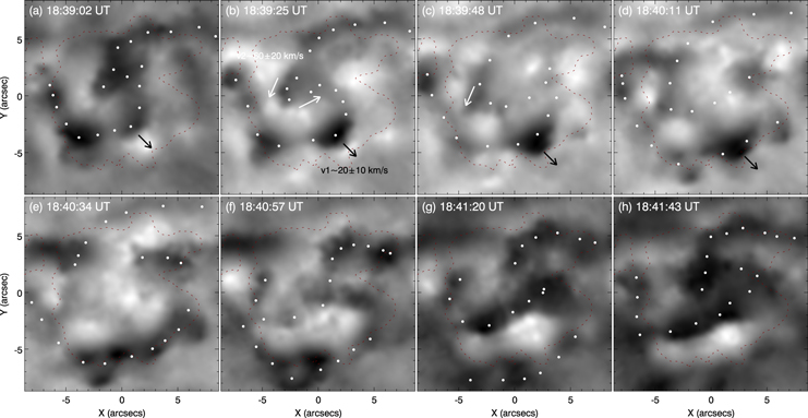
Figure 7. Temporal sequence of the two-armed spiral of one WF in sunspot 2. As usual, the red dotted lines outline the umbral boundary and the white solid circles highlight the WF trajectory. The black arrows display outward expansion of one spiral arm and the white ones show the WF core rotating anticlockwise.
Download figure:
Standard image High-resolution imageAnticlockwise rotation of the central patch becomes clockwise rotation after 18:55:43 UT. Figures 8(a)–(f) display this rotating motion. A dark ribbon arises at the left side of the umbral boundary of sunspot 2 in panel (a). Its head then rotates clockwise, and jumps to the umbral center as shown in panels (b) and (c) (see white arrows). The shifting velocity is more than 100 km s−1, which is too large to believe that this is a real rotating motion. Finally, a three-armed spiral structure emerges as shown in panel (e). However, we find that the three-armed structure is not a periodic phenomenon. It evolves toward an opposite pattern (anticlockwise rotation) after 1.5 minutes as shown in panel (g). Also, the three-armed spiral structure turns into a two-armed structure. In panel (i), a dark bump (shown by the white arrow) emerges. Its core exhibits fast rotation with a speed of ∼90 km s−1 during 19:00:53 UT–19:01:16 UT. Finally, another two-armed spiral structure appears in the umbra as shown in panel (l). Hence, we show again that the two-armed spiral structure arises periodically. In this case, the appearance period  according to the time interval between panels (g) and (l), and the radial velocity
  km s−1 (shown in panel (j)) is nearly the same as those values in Figure 7.
In summary, from Figures 3–8, the WFs display a common character in which the outer arms of the spiral structures expand radially and they become the penumbral waves upon travelling across the umbral boundaries. Therefore, our observations support the view that both umbral and penumbral waves have a common source in the photosphere and/or subphotosphere (Zhugzhda et al. 1984; Christopoulou et al. 2001; Rouppe van der Voort et al. 2003; Bloomfield et al. 2007; Tziotziou et al. 2007). However, our studies do not support a prevalent view that the difference between them arises from their propagation along differently inclined field lines. Figures 3–6 clearly show that they propagate together and separate only at the wave reflection points close to LBs. This indicates that they propagate along the same inclined field lines in the umbrae of the two sunspots. Furthermore, their radial propagation velocities are likely to be introduced by the disturbances propagating upward along the inclined field lines, which expand quickly in the radial direction.
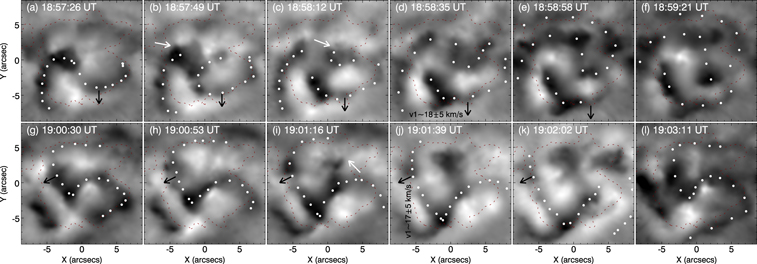
Figure 8. Similar to Figure 7, but for a clockwise rotating three-armed spiral evolving into a two-armed spiral rotating anticlockwise.
Download figure:
Standard image High-resolution image3.4. Spectral Features of the Umbral WFs
Figure 9 compares the filtered images at  Å in panels (a) and (d) with those at
  Å in panels (b) and (e) for U3 of sunspot 1 and sunspot 2. It appears that the blue wing images are negative images of the red wing. The figure also presents the Hα profiles averaged over the above respective entire FOVs and their filtered profiles averaged over the regions, i.e., r1 and r2 in panel (c) and r3 and r4 in panel (f). For the Hα profiles, the intensities in red wings are slightly higher than those in blue wings. The filtered profiles are antisymmetric, analogous to those of Stokes V-profiles. The LOS velocities averaged over r1 and r3 are −2.4 and −2.8 km s−1, and those over r2 and r4 are −0.4 and +0.6 km s−1, respectively. This indicates that the black (bright) patches in the filtered
  Å (
Å ( Å) images are strongly associated with the perturbations in the region of upward compression, while the bright patches do not always correspond to the perturbations in downward compression (see further discussions in the
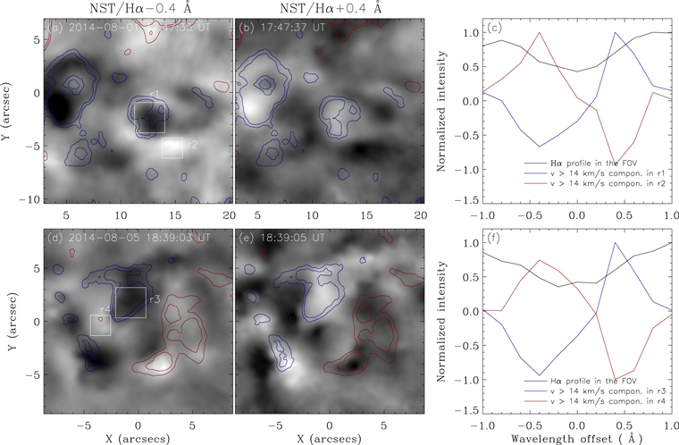
Figure 9.
 km s−1 filtered signals as seen from the blue wing −1 Å to the red wing +1 Å of the Hα spectral line. The filtered images at
  Å are shown in (a) and (d), and those at
  Å in (b) and (e). The blue/red contours represent the Hα LOS velocity with levels of −2.5 and −2.0 km s−1/+0.5 and +1.0 km s−1. (c) and (f) show the respective Hα profiles averaged over the overall FOVs of panels (a) and (d) (black), and the filtered profiles averaged over the square regions of r1 and r3 (blue) and over r2 and r4 (red).
Download figure:
Standard image High-resolution imageThe top panels of Figure 10 show the temporal evolution of the Hα line, which is obtained by averaging over regions r1 and r3 (in Figure 9). Both the original and filtered signals show the same sawtooth behavior, that is, a slowly increasing redshift followed by a rapid blueshift. This indicates the presence of upward-propagating magnetoacoustic shock waves (e.g., Lites 1986; Centeno et al. 2006; Chae et al. 2014; Tian et al. 2014; Yurchyshyn et al. 2014). The middle two panels display the corresponding temporal sequences of the averaged Hα intensity and LOS velocity over the same regions, where the velocities also show the sawtooth patterns (Centeno et al. 2009; Bard & Carlsson 2010; Tian et al. 2014; Yuan et al. 2014). The cross-correlation in panel (h) shows that there is a dominant peak at the time lag of 0 minutes, suggesting that the major oscillation signals of intensity and Doppler velocity are in phase. Thus, the major waves in r3 of sunspot 2 are upward-propagating. However, in panel (g) there are four peaks with nearly the same correlation at the lag times of −2.3, −1.0, 0.0, and 1.5 minutes. The averaged oscillation period is ∼2.4 minutes in r1 of sunspot 1 seen from panel (e). Thus, the positive peaks indicate that the waves upward are propagating (with phase delays of ∼2π or 0), while the negative peaks indicate that the waves are downward-propagating (with phase delays of ∼π).
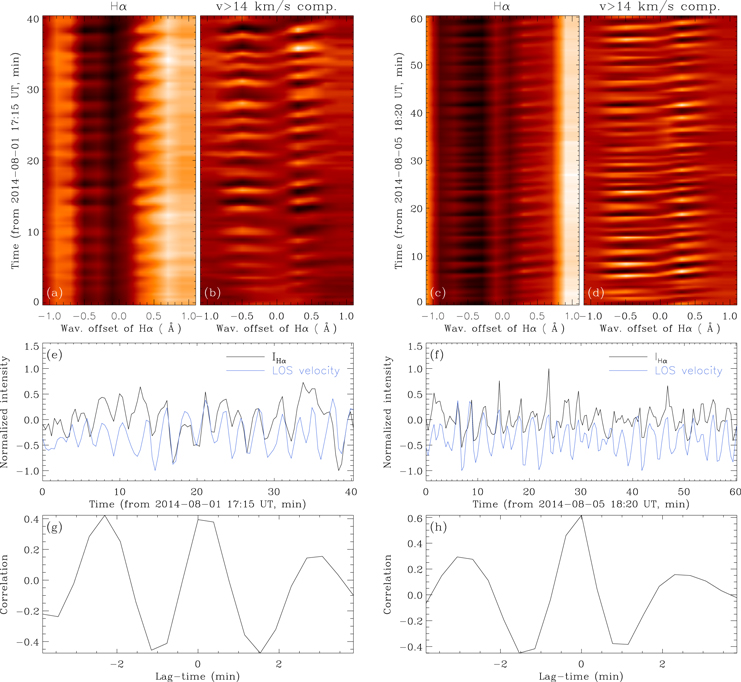
Figure 10. Shock waves in the central patches of umbrae. The wavelength–time maps of the Hα spectral line averaged over r1 and r3 in Figure 9 are shown in panels (a) and (c) for sunspots 1 and 2, respectively, and their filtered maps of  km s−1 are shown in panels (b) and (d). The temporal sequences of the averaged Hα intensity and LOS velocity over r1 and r3 are shown in panels (e) and (f), respectively, and the corresponding cross-correlation coefficient of the two as a function of time lag is shown in panels (g) and (h).
Download figure:
Standard image High-resolution image3.5. The Properties of the Umbral WFs at Different Heights
In the filtered  km s−1 images of He i 10830 Å in sunspot 2, we also find spiral structures of the umbral WFs. The same is found in the difference images of the 304 Å channel of SDO/AIA (which have been filtered with a frequency window of 3 mHz centered at 5.55 mHz). Figure 11 presents such an example as seen at different lines:
  Å, He i 10830 Å, and 304 Å in the umbra of sunspot 2.
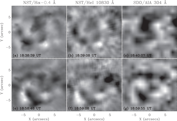
Figure 11. WF spiral structures at different heights as seen in the filtered images. Left and middle panels: the phase-speed filtered images of  km s−1 taken at
  Å and the He i 10830 Å spectral lines, respectively. Right panels: the difference images of AIA 304 Å, which have been filtered with a frequency window of 3 mHz centered at 5.55 mHz.
Download figure:
Standard image High-resolution imageFollowing Sych & Nakariakov (2014), we also study the phase relationship among the WFs at three altitudes by calculating 2D cross-correlation functions of the selected eight pairs of  Å and He i 10830 Å images, and eight pairs of He i 10830 Å and 304 Å images in the period of 18:36 UT–18:60 UT, which is shown in Figure 12. This shows that the gradient between
  Å and He i 10830 Å is larger than that between
  Å and 304 Å. We obtain two sets of time-lag data (corresponding to the local maxima of the 2D correlation function) of the umbral waves propagating from the formation height of
  Å to that of He i 10830 Å then to 304 Å. The averaged values are obtained by computing their means and variances, which are
  between
  Å and He i 10830 Å and
  9 s between
  Å and 304 Å. The time lags are consistent with a scenario of upward-propagating slow waves. In addition, assuming that the propagating velocities
  ∼ 15 km s−1 in the chromosphere (
 K) and 33 km s−1 in the transition region (
 K for 304 Å), we can estimate the difference in height of line formation between
  Å and He i 10830 Å
  km, and the difference between He i 10830 Å and 304 Å
  km.
km.
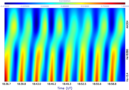
Figure 12. 2D cross-correlation function for the selected eight pairs of  Å and He i 10830 Å images, and eight pairs of
  Å and 304 Å images in the period of 18:36−18:60 UT.
Download figure:
Standard image High-resolution imageAbove a sunspot, White & Wilson (1966) estimated that the Hα spectral line forms at a height of 1500 km. Recently, the average formation height of Hα was found to vary between 1100 and 1900 km depending on the local optical depth (Leenaarts et al. 2012). The sunspot umbra is dark and well defined, suggesting that the opacity is greatly reduced and that the formation height may be as low as 1100 km (Jess et al. 2013). With the two lines of Si i 10827 Å and He i 10830 Å Centeno et al. (2009) detected that the height difference between the umbral photosphere and chromosphere is 1000 km. Therefore, if the formation height of Hα above the umbra of a sunspot is taken as 1100 km (even lower at  Å), then we infer that the He i 10830 Å line may form at ∼1360 km in the umbral chromosphere, which is slightly less than the 1500 km obtained by Centeno et al. (2009).
3.6. Distribution of Power Within the Spiral Structure
With a Morlet wavelet (Torrence & Compo 1998) applied to the  Å images, we obtain the spatial distributions of the narrow-band powers of the spiral structures of umbral WFs for sunspots 1 and 2 as shown in Figures 13 and 14, respectively. The 95% confidence threshold is used for the time series of periods at each pixel. Note that the power maps are further smoothed over a smoothing width of 30 pixels for the FOVs of 420 × 420 pixels in sunspot 1 and 600 × 600 pixels in sunspot 2.

Figure 13. Spatial distribution of the narrow-band power of one WF spiral structure in U3 of sunspot 1 at 17:49:29 UT on August 1. The red dotted lines have the same meaning as before, and the white circles outline the trajectory of the WF, with white arrows marking its head or tail.
Download figure:
Standard image High-resolution imageThe power distributions of umbral oscillations are quite complicated and each has its own features. In Figure 13, we take U3 of sunspot 1 as one example to show the power maps of a one-armed spiral structure at different frequencies. Panels (a) and (b) show that the WF head and tail (marked by the two arrows in panel (a)) have stronger power in the high-frequency ( minutes) oscillations. With frequency decreasing, some power patches (marked by the white arrows) gradually get enhanced (before P = 4.4 minutes) with distance in the direction opposite to the trajectory of WF propagation (in a clockwise direction). We propose that short-period waves evolve into shock waves over much smaller distances than long-period waves. With the high-frequency power dissipation, the lower-frequency oscillations dominate.
Figure 14 shows another example in the umbra of sunspot 2. The first two panels show that the high-frequency ( minutes) oscillations do not appear in the central patch of the two-armed spiral structure (marked by the white arrows) or in their spiral arms. This is not consistent with the study of Sych & Nakariakov (2014), who reported that the central patch of one two-armed spiral of a WF corresponds to high-frequency oscillations (e.g., P = 1.7 minutes). Panels (c)–(e) of Figure 14 show that the power of the spiral structure is mostly associated with the 3 minute oscillations (
 minutes). However, stronger power is concentrated not in its central patch, but in its arms or the regions marked by the two arrows in panel (d) (where the brightening regions shown in panel (b) of Figure 7 are). In particular, panel (e) shows four patches (marked by white arrows) concentrating near the umbra–penumbra boundary, whose distribution is analogous to magnetic oscillations with the signature of a whispering gallery-like mode of slow body waves in a thick magnetic flux tube (Zhugzhda et al. 2000; Staude 2002). In panels (g) and (h), as expected, the spiral structure in the umbra is unrelated to the lower-frequency (
 minutes) oscillations.
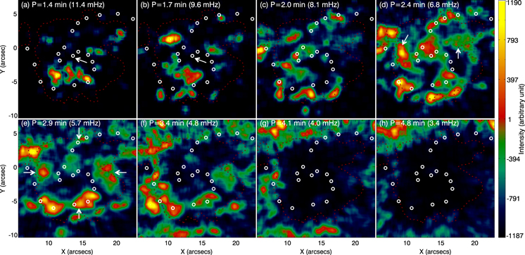
Figure 14. Similar to Figure 13, but for sunspot 2 at 18:39:25 UT on August 5.
Download figure:
Standard image High-resolution image4. DISCUSSIONS
In this study we have mainly utilized high-speed ( 14 km s−1) filtered images to investigate some properties of umbral oscillations. The validity of this filtering method has been tested with observed data as shown in the
  km s−1 so that we can distinguish the umbral and penumbral waves in the velocity distribution.
One of our important findings is that one-armed spiral structures of the umbral WFs are found in sunspot 1 and two- and three-armed ones in sunspot 2. We have tried to discover the relationship between the spiral structures and the twist of magnetic field. For sunspot 1, by checking the HMI white-light data we find that the four umbrae move as a whole and rotate anticlockwise, while their individual behaviors differ; for example, U1 and U2 rotate anticlockwise and U3 rotates clockwise. Because sunspot 2 has only one umbra, we can clearly see its motion in the time–space diagrams as shown in Figure 15, where two circular slits are marked in panel (a). We can see that there is no apparent rotation in the umbra, whereas in the penumbra both clockwise and anticlockwise rotations are found at the polar angles of  and
and  , respectively, which may come from tiny disturbances in the umbra where some imprints are seen at the corresponding positions.

Figure 15. Rotations of sunspot 2 in two days (through August 5−6). Panel (a): a HMI white-light map for the sunspot. Panels (b) and (c): two time–azimuth diagrams for the two virtual slits (the white circles on panel (a)) in the umbral and penumbral regions, respectively.
Download figure:
Standard image High-resolution imageSince WFs in the umbrae U1 and U2 are always clockwise rotations, which are opposite to the umbrae's own anticlockwise rotations, this indicates that the twist has little or no effect on the one-armed spiral structure in U1 and U2. However, it is hard to draw the same conclusion for U3 because the rotation and twist directions are the same. We have already shown that in sunspot 1 the change in the WF direction occurs at the reflection points near those umbral–penumbral boundaries close to LBs (blue arrows in Figures 3–6). Therefore, we conjecture that the spiral structures in sunspot 1 are produced by their inward reflections at the umbral LBs. However, we should treat this conjecture with particular caution as the topology of sunspot 1 was quite complex.
In sunspot 2, the multi-armed spiral structures alternate between clockwise and anticlockwise rotation. This opposite rotation may come from the opposite vortices relating to the magnetic fields. At least, we cannot exclude the association of the multi-armed spiral structures with the twist of the magnetic field. This result is different from the result of Sych & Nakariakov (2014), who found no twisted magnetic field in a two-armed spiral structure.
One should note that the WF spiral structures in the umbrae of the sunspots provide a clue to discern the constitution of sunspots between the proposed monolithic (Cowling 1953) and spaghetti models (Parker 1979). The two- or three-armed (uniform) structures of the WF trajectories in sunspot 2 indicate that they are produced by the interaction between multiple strands of flux tube and the slow magnetoacoustic waves under the photosphere. Those in the three umbrae of sunspot 1 displayed that the waves propagated and sometimes were reflected, likely in the three monolithic flux tubes. Rempel (2011) suggested that sunspots that present light bridges and signs of flux separation are more spaghetti-like than those without LBs. Therefore, we conjecture that the main umbra of sunspot 1 may also consist of multiple strands.
5. CONCLUSIONS
The principal aim of this work was to investigate the running waves in the two sunspots observed on 2014 August 1 and 5. The main results are as follows.
(1) The phase-speed filters are used to extract the fast rotating structures in the Hα images (mainly at the −0.4 Å passband). We demonstrate that the filtered images of  km s−1 may be suitable for studying umbral waves and the images of
  km s−1 for studying penumbral waves.
(2) The umbral WFs emerge and propagate both radially and azimuthally in sunspots 1 and 2. When the WFs arrive at the umbral boundaries, some of them may become the penumbral waves and continue to propagate in the radial direction. We conjecture that the umbral and penumbral waves are possibly excited by a single common source.
(3) The one-armed spiral structures of the WFs in sunspot 1 may be produced by waves reflected at the LBs. The multi-armed spiral structures in sunspot 2 are likely related to the twist of the magnetic field under the photosphere. Moreover, its stronger oscillating power prefers to concentrate at the umbral–penumbral boundaries.
(4) The spiral structures of WFs appeared sequentially at different heights in the solar atmosphere, which confirms previous studies that the 3 minute umbral disturbances are p-mode waves propagating upwards along magnetic field lines in the umbra of a sunspot.
However, the complex topology of sunspot 1 means that we need observations with higher resolution and higher cadence to confirm our results.
We thank the anonymous referee for his/her valuable comments, which have enabled us to improve the quality of the presentation. This work is supported by the strategic priority research program of CAS with Grant No. XDB09000000 and the other Grants: National Basic Research Program of China under grant 2011CB8114001, XDB09040200, 11373040, 11373044, 11273034, 11303048, 11178005, 11573012, AGS-0847126, and NSFC-1142830911427901. BBSO operation is supported by NJIT, US NSF AGS-1250818, and NASA NNX13AG14G, and NST operation is partly supported by the Korea Astronomy and Space Science Institute and Seoul National University, and by the strategic priority research program of CAS.
APPENDIX: PHASE-SPEED FILTER
A filtering method that works in the frequency–wavenumber ( ) domain is used to extract the wave signals of interest from the analyzed temporal sequences of Hα images. Specifically, a three-dimensional time–space matrix generated by one image sequence is transformed to the
  domain using the three-dimensional Fourier transform. The wave phase velocity, v, is equal to the ratio of ω and k in the
  domain. A vertical cone symmetric about the ω axis can cut off all velocity components outside the cone and leave unchanged all components inside. The Butterworth filter is applied to reduce ringing and wrap-around error, and its low- and high-pass functions are given by

and

respectively, where vc is the cut-off velocity and n is the order. If we are interested in some special components within a certain speed range, then a band-pass filter is needed, whose function is  , created by combining a low-pass filter with a high-pass filter. Finally, with an inverse transform of the FFT, the required images in the spatial domain are obtained. In the paper, the temporal sequences of images are filtered according to the following three speed regimes:
  km s−1 (high-pass), 4 km
  km s−1 (band-pass), and
  km s−1 (low-pass).
However, as umbral waves are the main concern of this study, we pay much attention to the low-pass filter (see Section 3.1) and apply it to all the temporal sequences of Hα images from −1 to +1 Å off the line center. After comparisons, we find that the waves are clearly seen in the filtered images at the blue wing −0.4 Å. Therefore, they are mostly investigated at this passband as shown in Figures 3–8. The filtered components in the red wing +0.4 Å seem to be negative images of those at −0.4 Å shown in Figure 9. To investigate the umbral oscillations evolving in the whole Hα line, we obtain the temporal sequences of the averaged values over the umbral center of U3 in sunspot 1 and that in sunspot 2 (the square areas r1 and r2 shown in Figure 9) at each passband of the Hα line and stack them together in ascending order of wavelength as shown in Figure 10. We also apply the filtering method to the He i 10830 Å images of sunspot 2, and the detected umbral WFs are shown in Figure 11 similar to those at  Å.
Å.
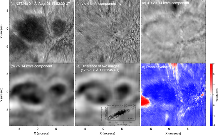
In Figure 16, we test the validity of the filtering methods on the observed data from 2015 August 1. Panel (a) presents a Hα −0.4 Å image at 15:52:30 UT. Its filtered images in three velocity regimes are shown in panels (b)–(d). Panel (e) exhibits a difference image obtained from the Hα −0.4 Å image at 15:52:08 UT by subtracting its preceding one at 15:51:45 UT. It resembles the low-pass filtering image (panel (d)), i.e., dark umbral cores surrounded by bright rings. Note that the image in panel (e) (with a FOV of 420 × 420 pixels) has been smoothed over a large smoothing width of 50 pixels. The inset of panel (e) shows that the correlation between the filtered (panel (d)) and difference (panel (e)) images is moderately high, up to 0.86. From this comparison, we prove the reliability of our filtering method.
Figure 16. Test of the phase-speed filters with the data from 2014 August 1. Panels (a)–(d) in order: A H Å image and its filtered images of
  ,
,  , and
, and  km s−1, respectively. Panel (e): a difference image of the two
  Å images at 17:52:08 UT and 17:51:45 UT, on which the inset is a comparison plot for the filtered and difference signals. Panel (f): Hα LOS velocity.
Download figure:
Standard image High-resolution image
To investigate the causes of bright and dark patches in panel (d), we show a map of Hα LOS velocity at 15:52:30 UT in panel (f). It is found that the dark patches in the umbral cores correspond to stronger disturbances in a phase of upward compression, while their surrounding bright patches correspond to much weaker disturbances, possibly also in upward compression (as the averaged velocity is often negative in these regions). Moreover, for the difference image of panel (e), the dark patches mean that the following image in those regions is darker than the preceding one, or vice versa. Therefore, combining the LOS velocity map and the difference image, we deduce that the dark patches in panel (d) are caused by the umbral waves emerging and expanding in the regions, and the bright ones by the WFs just moving out of those regions. The low-pass filtered images can record these fast, transversely moving structures (with  km s−1).