


ABSTRACT
A long-established goal of solar physics is to build understanding of solar eruptions and develop flare and coronal mass ejection (CME) forecasting models. In this paper, we continue our investigation of nonlinear forces free field (NLFFF) models by comparing topological properties of the solutions to the evolution of the flare ribbons. In particular, we show that data-constrained NLFFF models of three erupting sigmoid regions (SOL2010-04-08, SOL2010-08-07, and SOL2012-05-12) built to reproduce the active region magnetic field in the pre-flare state can be rendered unstable and the subsequent sequence of unstable solutions produces quasi-separatrix layers that match the flare ribbon evolution as observed by SDO/AIA. We begin with a best-fit equilibrium model for the pre-flare active region. We then add axial flux to the flux rope in the model to move it across the stability boundary. At this point, the magnetofrictional code no longer converges to an equilibrium solution. The flux rope rises as the solutions are iterated. We interpret the sequence of magnetofrictional steps as an evolution of the active region as the flare/CME begins. The magnetic field solutions at different steps are compared with the flare ribbons. The results are fully consistent with the three-dimensional extension of the standard flare/CME model. Our ability to capture essential topological features of flaring active regions with a non-dynamic magnetofrictional code strongly suggests that the pre-flare, large-scale topological structures are preserved as the flux rope becomes unstable and lifts off.
Export citation and abstract BibTeX RIS
1. INTRODUCTION
Solar flares are the most energetic events in the solar system. During a flare, magnetic free energy is converted to heat, radiation, and kinetic energy (bulk flows and energetic particles) in the process of magnetic reconnection (see review by Forbes et al. 2006). Solar flares emit at all wavelengths, but their most notable effects are in the EUV and X-rays, where the flare radiation can be several orders of magnitude larger than the pre-flare emission (Fletcher et al. 2011). Flares are often accompanied by coronal mass ejections (CMEs), and together they present the strongest drivers of space weather in the solar system and specifically in the geospace environment.
Flares and CMEs produce many observed features in different layers of the solar atmosphere, from the photosphere to the corona and solar wind. The two-dimensional (2D) standard flare model (Carmichael 1964; Sturrock 1966; Hirayama 1974; Kopp & Pneuman 1976; Shibata et al. 1995; Tsuneta 1996, 1997) is quite successful at explaining the main flare features observed in the atmosphere of the sun. The 2D model was extended to three dimensions by Aulanier et al. (2012) and Janvier et al. (2013), and is schematically represented in Figure 1. It generally requires the presence of a flux rope (gray twisted field lines), which is destabilized by a mechanism, which is yet not fully known. Reconnection takes place under the flux rope, which powers the flare and indirectly creates the flare ribbons (yellow), the hot cusp-shaped loops (green), and the flare loop arcade (blue). The flare loops represent reconnected field lines and the ribbon emission originate at the footpoints of the flare arcade by heat conduction and particle flows (Fletcher et al. 2011) down the reconnected field lines from the reconnection site (marked as dotted arrows). When the heat and particles encounter the chromosphere they create an evaporation flow (marked as dashed arrows) driven by the pressure gradient (Antonucci et al. 1984), which populates the flare loops with hot plasma and makes them emit in UV and soft-X-ray. The coronal volume around the footprints of the expanding flux rope is depleted in density and shows up as transient coronal holes (CH) or dimmings, which are the coronal source manifestation of the CME. The corresponding observed features are displayed on the figure as well. This is the mechanism for producing classical two-ribbon flares that are associated with flaring under a flux rope. The flux rope may not erupt fully and still produces a two-ribbon flare as long as conditions for reconnection exist under the flux rope.

Figure 1. Standard flare cartoon. The expanding flux rope is shown in gray; the QSL cross section in the plane perpendicular to the flux rope with the HFT is given in red; the newly reconnected cusped field line is green; a field line from the flare arcade is shown in blue, and the footpoints of the flare arcade are shown in yellow. The standard flare cartoon is accompanied by images from the main space observatories showing the observed features explained by the model: (a) CME with three-part structure from SOHO/LASCO; (b) cusped-shaped loop from Yohkoh/SXT; (c) transient CHs from SDO/AIA; (d) flare arcade from TRACE; and (e) flare ribbons from Hinode/SOT.
Download figure:
Standard image High-resolution imageThe relationship of S-shaped (sigmoidal) loops seen in Yohkoh/SXT (Tsuneta et al. 1991) soft-X-ray observations with flares and CMEs dates back to the work of Rust & Kumar (1996) and Canfield et al. (1999). Higher resolution observations from the X-ray telescope on Hinode/XRT (Golub et al. 2007) have allowed us to follow the energy build-up in sigmoidal active regions. McKenzie & Canfield (2008) related the evolution of AR loops seen in XRT to the Titov & Démoulin (1999) flux-rope model. They noticed that the active region evolved from a two-J-shaped loop configuration to a single S-shaped configuration. This insight has led to detailed comparisons between observations and idealized models (Archontis et al. 2009; Aulanier et al. 2010), and to the type of detailed comparisons between data-driven models and dynamic observations that we present in this paper. The structure and evolution of sigmoidal active region can be captured by nonlinear force-free field (NLFFF) models that correctly identify the location of the stability boundary (Kliem et al. 2013).
The three-dimensional (3D) dynamical MHD simulations of Aulanier et al. (2012) and Janvier et al. (2013) were used to extend the standard flare model to three dimensions. In the model, reconnecting field lines slip through plasma (Aulanier et al. 2006) and their footpoints apparently move along the two-J-shaped quasi-separatrix layers (QSLs; see the yellow J-shaped regions in Figure 1). QSLs are 3D topological features over which the field line connectivity experiences drastic changes, but is nonetheless continuous, unlike 2D separatrices. The concept of QSLs was introduced by Priest & Démoulin (1995) and Démoulin et al. (1996), and extended by Titov et al. (2002) and Titov (2007). In the standard 3D model the flux-rope-associated QSLs overlay strong current concentrations in the photosphere, which are the extensions of the coronal currents. The 3D models, unlike the 2D ones, predict that the flare ribbons, current concentrations, and QSLs at the photosphere are all closely related, with basically the same shape, size, and location. These findings motivated paper I (Savcheva et al. 2015), this study, and the studies of Janvier et al. (2014) and M. Janvier et al. (in preparation). Janvier et al. (2014) already demonstrated the correspondence between flare ribbons and photospheric currents derived from vector HMI magnetograms during an X-class flare, and M. Janvier et al. (in preparation) shows the match between low-lying QSLs and current ribbons in another X-class event.
In the 3D model, the flux-rope-binding QSL crosses itself under the flux rope, creating a subvolume with the highest connectivity change, called a hyperbolic flux tube (HFT; Titov et al. 2002). The accepted measure of QSL strength is the the squashing factor, Q (Titov et al. 2002; Titov 2007). The HFT is located at the largest value of Q in the volume. In the 3D standard model the legs of the HFT bind the domain where the flare arcade loops appear. There are field lines coinciding with the legs of the HFT and these outermost field lines are the first ones to reconnect. Thus, the outer edge of the ribbons should coincide with the flux-rope-related QSLs (in cross section given in red in Figure 1). In Paper I, we demonstrated this correspondence for seven different regions with QSLs derived from marginally unstable magnetic field models based on the flux-rope insertion method. Some recent work (Sun et al. 2013; Liu et al. 2014; Vemareddy & Wiegelmann 2014; Zhao et al. 2014) shows the existence of QSLs in the vicinity of flare ribbons for two complex magnetic configurations derived from nonlinear NLFFF extrapolations. Masson et al. (2009, 2014) demonstrated the close correspondence between circular QSLs and flare ribbons in a null point configuration from an NLFFF extrapolation. Similar results are also found by Su et al. (2009) and M. Janvier et al. (in preparation) using the flux-rope insertion method.
Paper I and the present study are logical continuations of the results obtained in Savcheva et al. 2012a (hereafter S12). We showed that a flux rope obtained from NLFFF modeling with the flux-rope insertion method is outlined by QSLs that quasi-separate it from the overlying arcade. Based on the static NLFFF modeling and the idealized dynamical MHD simulation of Aulanier et al. (2010), we put forward a scenario for eruption based on a positive feedback between reconnection under the expanding flux rope and the torus instability. Although in this study we are not concerned with the cause of the destabilization of the flux rope, we summarize this scenario for completeness, since it is at the basis of the modeling that we perform in the current study. In our scenario, the two-J-shaped field lines that comprise sigmoidal active regions reconnect at an HFT under the flux rope. Due to the inverse relationship between the thickness of the QSL and the value of Q as well as the relation between the thickness of QSLs and the accumulated current sheets at their locations (Démoulin et al. 1996; Aulanier et al. 2005, 2006), the HFT is the place where the thinnest current sheets can accumulate in the presence of footpoint motions, and thus facilitate reconnection. In Savcheva et al. (2012c), we demonstrated that indeed an HFT appears at the locations of flares a few hours before the flare, hence the HFT is the most probable site for flare reconnection (see also Zhao et al. 2014). The product of the reconnecting two-J-shaped field lines is a long S-shaped field line that adds to the flux of the flux rope, and a flare arcade field line that lies in the domain under the HFT. The build-up of S-shaped field lines causes the flux rope to expand and elevate until at some height it reaches the torus instability domain. The torus instability occurs when the the overlaying potential arcade decays with a critical index,  depending on the flux-rope geometry and shear in the overlaying arcade (Kliem & Török 2006; Démoulin & Aulanier 2010). In this process the tension of the arcade is not sufficient to restrain the expanding flux rope. Hence, the instability allows it to grow and elevate even more, which subsequently elongates and thins the reconnection current sheet further and causes more reconnection to take place. This scenario accounts for the slow rise of filaments based on tether-cutting-like reconnection (Moore et al. 2001) and the fast eruption after the torus instability kicks in.
In the classical two-ribbon flare, ribbons display two kinds of motions (Asai et al. 2002, 2004; Fletcher 2009; Qiu 2009; Qiu et al. 2010). One is a "zipper" motion (fast elongation) parallel to the polarity inversion line (PIL) during the impulsive phase of the flare with velocities of 10–100 km s−1. The other is an expanding (separating) motion perpendicular to the PIL during the gradual phase of the flare with velocities of 1–20 km s−1. Another common motion, mostly visible in the footpoints of flare loops, is the strong-to-weak shear transition (Su et al. 2006, 2007; Aulanier et al. 2012). Overall, the spatial pattern of the flare ribbons can be quite complex and intermittent (Krucker et al. 2003; Asai et al. 2004; Bogachev et al. 2005; Qiu et al. 2010). The expanding motion is readily explained with the standard flare reconnection model: reconnection under the flux rope creates the flare ribbons, and as the flare site lifts up, more and more flux reconnects and creates loops with footpoints that are farther away from the PIL. Thus, this kind of motion is an apparent motion rather than an actual one. However, in order to understand the zipper motion and the strong-to-weak shear transition, a 3D flare model is needed.
Observations have shown the following properties of the ribbon motion (Qiu et al. 2002, 2010; Qiu 2009): (1) Ribbons move faster in low magnetic flux regions due to conservation of flux, i.e., both ribbons should sweep up the same amount of flux on both sides of the PIL, which also equals the total reconnected flux. Hence, the ribbon in the low flux region should move faster. (2) The ribbons in the lower flux region are generally brighter than these in the high flux region. This is explained by the magnetic mirror effect of the magnetic field on the particles streaming down from the reconnection site. In the higher flux region, the particles' mirroring is stronger, and hence they spend less time interacting with the dense chromosphere, thus producing less ribbon emission. Although the resemblance of QSLs and ribbons has been demonstrated before from idealized MHD simulations (Schrijver et al. 2011; Janvier et al. 2013), the current concentrations in the photosphere have been matched to ribbons (Janvier et al. 2014), and the QSLs in complicated active regions have been shown to lay close to the ribbons, (Liu et al. 2014; Zhao et al. 2014; Dalmasse et al. 2015; Savcheva et al. 2015), and the QSLs have always been visualized as static topological features over the duration of the flare. However, as the quasi-connectivity domains are evolving in time thanks to reconnection, so are moving the linked topological structures. The shape and position of the QSLs are thus evolving as shown in numerical simulations (Aulanier et al. 2006; Janvier et al. 2013). However, the displacement of QSLs in link with the motion of observed flare ribbons has never been shown.
In this paper, we study three accurate magnetic field models of sigmoidal active regions that produce two-ribbon flares. The pre-flare evolution and the flaring dynamics are well observed by AIA. We produce unstable magnetic field models of the 3D coronal structure using the magnetofrictional flux-rope insertion method (van Ballegooijen 2004) by adding some additional axial flux to the best-fit model. The unstable models are not force-free and continue to expand and rise as we iterate, which is the main feature we make use of in this paper. We perform topology analysis based on these models over the evolution of the flux ropes. In Paper I, we have shown that the chromospheric footprints of the flux-rope QSLs match the flare ribbons at the first instance when the ribbons appear in full length; here we look at the motion of the flare ribbons and flare loops in the context of the unstable flux-rope topology. All NLFFF models of active regions are approximations of the solar fields. Our confidence in the models depends on the ability of a single solution to fit a wide range of observational constraints. Flare ribbons are the main and the most straightforward observable informing us on the flaring magnetic field geometry. The ability to reproduce the position, shape, and evolution of flare ribbons is an essential step in our capability to properly model the dynamics of an eruption and the launch of a CME. The results we present here are novel and represent a significant step forward in the ability to predict solar eruptions.
The paper is organized as follows: In Section 2 we present the observations of the different flare regions in all three cases. In Sections 3.1 and 3.2 we describe the details of the magnetic field modeling, and in Section 3.3 we present the QSL calculation and topology analysis. The supporting results of the evolution of the flux ropes and their currents is given in Section 4. The main results on the evolution of the flare ribbons and corresponding QSLs are presented in Section 5.1 and the flare loops and strong-to-weak shear transition is given in Section 5.2. The summary and conclusions are given in Section 6.
2. OBSERVATIONS
In Paper I, we had chosen seven regions, two from the pre-SDO era, one during an AIA X-class flare with largely saturated ribbons, and one with a significant gap in the AIA data covering the ribbon evolution. Thus, for the present study we were left with three suitable regions that have AIA observations with good quality covering the ribbon dynamics and flare arcade evolution in great detail. The data sets consist of almost all AIA wavelengths (Lemen et al. 2012; 1600, 304, 211, 193, 211, 335, 131, and 94 Å) as well as HMI line of sight (LOS) data (Scherrer et al. 2012). The high cadence of AIA (12 s) and the multiple channels allow us to have good coverage of the dynamics of the event at different temperatures and parts of the solar atmosphere.
2.1. The SOL2010-04-08 Sigmoid
This event was studied extensively by Su et al. (2011), where they modeled it with the flux-rope insertion method and looked at its 3D magnetic field structure before and at the onset of the flare. The region produced a GOES B3.7 flare at 02:20 UT on 2010 April 08. This region appeared during the commissioning phase of SDO/AIA, so we were able to use AIA 335 Å images and HMI magnetograms to constrain the NLFFF models.
The flare ribbons are visible in most channels, except 94 Å, but the chromspheric 304 and 1600 Å channels are most suitable for studying the ribbons. The ribbons appear at 02:30 UT in AIA 304 Å and remain visible until 04:54 UT. Both ribbons first experience a zipper motion along the PIL to the east and west of the central part of the sigmoid until 03:04 UT. The zipper motion concludes with the ribbons wrapping around the two transient CHs. The largest ribbon spreading is observed in the middle of the sigmoid. Then, the ribbons display clear sideways motion away from the PIL as expected in the standard two-ribbon flare scenario. Snapshots of the ribbon evolution are shown in Figure 2 and in the bottom right panel we have color coded the ribbons by the time they appear showing their evolution.
Figure 2. Time sequence of AIA 304 Å images centered at the SOL2010-04-08 sigmoid. The spreading motion of the ribbons is clear in the first five panels. Another representation of the ribbon dynamics is shown in the last panel in the bottom right, where we have detected the ribbons and plotted their color-coded time evolution. Time progresses as shown in the color bar. The color-coded ribbons are plotted on top of the magnetogram used to produce the NLFFF model.
(An animation of this figure is available.)
Download figure:
Video Standard image High-resolution imageThis event displays very nicely outlined transient CHs, which can be seen in the upper left panel of Figure 3. The eastern CH appears at 02:59 UT in AIA 193 Å accompanied by an expanding loop to the east of it, and grows until 04:10 UT.The west transient CH appears at 03:09 UT, and grows until 04:08 UT. The eastern CH is round and more confined, while the western one is more spread out. The presence of transient CHs is an indication of the development of a CME, confirmed by LASCO observations of the event (Su et al. 2011).
Download figure:
Video Standard image High-resolution imageDownload figure:
Video Standard image High-resolution imageDownload figure:
Video Standard image High-resolution imageIn the middle of the region, where the flare ribbons appear, the first flare loops show up, which are seen in the 193 Å image in the upper left panel of Figure 3. The flare loops appear first in AIA 94 and 335 Å at 02:36 UT, and in AIA 193 Å they appear at 02:57 UT. The loops are at first more sheared and later they relax to a less sheared state. The shear of the flare loops is defined by the angle between the line that connects the two footpoints of the loops and the PIL. Predominantly, there are loops that connect the centers of the flare ribbons, but there are also loops that connect from the middle of the ribbon to the side lobes where the edges of the dimmings are.
2.2. The SOL2010-08-07 Sigmoid
This data set covers the period 17:00–21:00 UT on 2010/08/07, from an hour before the start of the M1 flare until after the last flare loops disappear. We also utilize XRT synoptic images and HMI magnetograms to constrain the NLFFF models.
First, a spiral-shaped flare ribbon appears at 17:53 UT in AIA 304 Å to the side of the sunspot in the region around position (−470'', 70'') on the first panel of Figure 4, associated with the lift-off of the top filament in this double-decker filament eruption (Kliem et al. 2014). This flare ribbon is not very dynamic and remains visible for most of the time. During the main event different portions of the the southern and northern flare ribbon appear at different times. The southern flare ribbon is seen in full length for the first time in Figure 4 at 18:05 UT and remains visible until 18:36 UT. The northern ribbon grows in length until 18:15 UT. During that time both the southern and northern flare ribbons move apart away from the PIL. Both ribbons remain visible until 20:18 UT.
Download figure:
Video Standard image High-resolution imageSeveral snapshots from the evolution of the ribbons are shown in Figure 4. The dynamical nature of the ribbons is shown in the bottom right panel of the figure, where we have overlaid a pre-flare 171 Å image with a color-coded evolution of the ribbons by time. From this figure it can be seen that the southern flare ribbon moves farther away from the PIL as compared to the northern one, which on the other hand shows more prominent elongation. It can be seen from the figure that while the southern ribbon covers a significant part of the positive polarity, the northern ribbon lies at the edge of the negative polarity. This ribbon evolution follows the previously observed behavior (Qiu 2009) that the ribbon situated in a more intense magnetic field moves a shorter distance away from the PIL than the one in the weaker field region.
Two transient CHs appear at 18:08 UT and grow until 18:10 UT in AIA 193 Å. Both CHs are offset with respect to the endpoints of the inserted flux rope, which closely follows the dark filament before the eruption, and the observed hooks (i.e., the hooks of the Js) of the flare ribbons. A potential cause of this offset could be a slipping motion (Aulanier et al. 2006) of the flux-rope footprint, similar to the case discussed in Jiang et al. (2012).
The first flare loops are seen as early as 18:05 UT in an XRT synoptic image, which is to be expected since loops appear first in the hottest channels, i.e., X-rays. The first AIA flare loops appear in AIA 94 and 335 Å at 18:06 UT. In AIA 171 Å the flare loops appear at 18:38 UT and a few loops remain visible until 20:56 UT. The flare loops show a clear strong-to-weak shear transition especially in the west part of the region, which is visible in the bottom two panels of Figure 3. Some loops reaching from the sunspot and connecting to the middle of the sigmoid show a significant shear for most of the time.
2.3. The SOL2012-05-08 Sigmoid
The region produced a C-class flare at 08:26 UT, as classified by GOES. We use XRT images and AIA 335 Å and HMI data to constrain the magnetic models discussed in the next section.
The region showed a clear sigmoidal shape in the days leading to the eruption and clear two-J-shaped flare ribbons as shown in Paper I. The ribbons appear at 09:27 UT in AIA 304 Å and remain visible until 12:59 UT. The eastern ribbon appears first in the very middle of the sigmoid and zips along the PIL to finally encompass the whole length of the filament at 09:35 UT. The motion of the flare ribbons is well observed by the high cadence of AIA. We use the 304 Å channel to track the motion of the ribbons, which move much farther apart in the northern part of the region, where the field is weaker. The ribbon evolution is shown in Figure 5.
Download figure:
Video Standard image High-resolution imageThe region shows a clear dimming region to the south of the arcade, which is visible between 10:17 UT and 11:07 UT in AIA 193 Å—it can be seen in the top right panel of Figure 3. It spreads from the southern footprint of the flux rope and to the west. The corresponding northern dimming is not visible possibly because it is overlaid with the bright flare loops and the remnants of the original loop system. The flare loops appear first at 09:35 UT in AIA 94 Å in the middle of the sigmoid and are significantly sheared. They are shown in the same image of Figure 3. The shear does not change significantly until they disappear at 12:29 UT.
This region displays an interesting change in the southern footprint of the filament. The filament that was visible for a couple of days before the flare had a clear S-shape. However, in the process of eruption the southern hook of the filament disappears and a new connectivity appears with the southern footprint located at the western end of the southern flare ribbon around (x, y) = (−50'', 200'') as can be seen in the bottom panels of Figure 5. As discussed in Paper I, this made the modeling of the flux-rope path in this region more challenging.
3. MAGNETIC FIELD MODELING AND TOPOLOGY ANALYSIS
3.1. Initial Magnetic Field Modeling
For all regions we have used the flux-rope insertion method as described in Paper I to produce NLFFF models for times preceding the eruptions by about one hour. We have already described the method in detail and demonstrated its usefulness in application to sigmoidal active regions and filament channels (Bobra et al. 2008; Savcheva & van Ballegooijen 2009; Su et al. 2011, 2015; Savcheva et al. 2012a, 2012b, 2012c, 2015; Su & van Ballegooijen 2012). The flux-rope insertion method is a magnetofrictional method that uses LOS magnetograms, such as those from HMI, and coronal observations of loops preceding the eruption to constrain the NLFFF models. In a nutshell, the method for producing NLFFF consists of the following steps: (1) A global potential field source surface (PFSS) model (Bobra et al. 2008) is computed based on a low-resolution synoptic SOLIS or HMI magnetogram. (2) A high-resolution region centered at the active region is selected from a 12 minute HMI magnetogram and a new modified potential field extrapolation is performed with side boundary conditions given by the global PFSS model. The bottom boundary is the LOS HMI magnetogram. The hires potential field is modified with two sources in the photosphere where the inserted flux rope is to be anchored. (3) A flux rope is inserted by modifying the initial vector potential ( where
where  ) with a given combination of axial and poloidal flux. (4) A grid of models is computed with different combinations of axial and poloidal flux. (5) The models are relaxed to a force-free state using magnetofriction (MF, see Section 3.2), when an equilibrium is reached between the pressure in the flux rope and the tension in the overlaying arcade. (6) Based on quantitative comparison (described in detail in Savcheva & van Ballegooijen 2009) of pre-flare coronal loop observations with disk-projected field lines from these models, we issue a best-fit model that closely matches the observed loop configuration in XRT and AIA 335 Å and 193 Å images.
Although in previous studies we were concerned with the best-fit models that represented the equilibrium coronal magnetic fields preceding flares, here we are more interested in dynamic flare features. The flux-rope insertion method assumes that all velocities in the corona must vanish in order to produce a stable relaxed model, but the method is still capable of producing unstable models. These models pass the threshold of stability by having more axial flux than the flux rope can contain and remain stably bound by the overlaying arcade. The flux rope in these unstable models continues to expand and rise in height with continued iterations. All unstable models show HFTs under the flux ropes in accordance with the scenario put forward in S12.
As detailed in Paper I, we added 1–2 × 10²⁰ Mx of axial flux to the best-fitting models to make them unstable since we have determined that the axial flux is mostly responsible for the stability of the configuration rather than the poloidal flux, to which our method is not very sensitive (Su et al. 2011).
In Table 1 we have given the times, tmag when the equilibrium pre-flare NLFFF models have been constructed, and input and output parameters of the used unstable models for all regions. We have also included the total unsigned flux in the region for comparison with the rest of the derived parameters. A summary of some best-fitting field lines obtained with this scheme are shown in Figure 6, bottom row, for the three sigmoids. The top row shows the corresponding XRT observations used to obtain these models. The qualitative match between the field lines in the bottom row and the loops in the X-ray images is apparent.
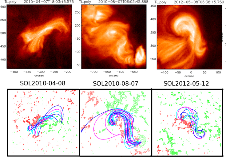
Figure 6. Top: XRT images at the time of the magnetic field models. Bottom: field lines traced from the corresponding best-fit marginally stable models for the three regions. The colors of the field lines are just used to distinguish the different field lines. The green and red contours represent the negative and positive polarities, respectively.
Download figure:
Standard image High-resolution imageTable 1. Model Parameters for All Regions Studied Here
| Time | Unsigned Flux in | Axial Flux | Poloidal Flux | Potential Energy | Free Energy |
|---|---|---|---|---|---|
| Region (1021 Mx) | (1020 Mx) | (1010 Mx cm−1) | (1031 erg) | (1031 erg) | |
| 2007/02/12 | 18.3 | 5 | 5 | 3.65 | 1.7 |
| 06:41 UT | |||||
| 2007/12/07 | 6.6 | 7 | 0.5 | 1.28 | 0.55 |
| 03:20 UT | |||||
| 2010/04/08 | 17.8 | 6 | 1 | 5.3 | 1.85 |
| 02:00 UT |
Download table as: ASCIITypeset image
For SOL2010-04-08 and SOL2010-08-07 we performed the modeling based on very well-constrained flux-rope path. However, the flux-rope path for SOL2012-05-08 was not constrained well since the filament observed in AIA 304 Å changed significantly in the process of eruption from its pre-flare S-shaped state. Consequently, we experimented with three different flux-rope paths for this region—one folloing the pre-flare S-shaped path, one following the path that was illuminated by the ribbons, and one that consisted of two flux ropes covering the path illuminated by the flare ribbons. Since the alternative second and third path did not give markedly better results, we chose to use the path constrained by the pre-flare S-shaped filament in order to be consistent with the models of the other regions.
3.2. Magnetofrictional Simulations
The flux-rope insertion method employs MF relaxation to obtain a sheared arcade or a flux-rope 3D coronal model. For the MF relaxation in the flux-rope insertion method, we use a mode of diffusion only (Mode 5), rather than the different modes of operation that include injection of horizontal fields from below. The boundary conditions stay the same throughout the MF process. The bottom boundary condition is fixed to be the LOS magnetogram, i.e., we only have the radial component of the magnetic field and no horizontal components during the whole relaxation. As the relaxation proceeds, the magnetic field volume evolves, but the boundary stays fixed, the field is forced to go to the LOS field at the photosphere, and no currents are permitted to cross the lower boundary. The side boundaries stay open, i.e., the field from the high-resolution box connects to the global potential field at the sides, and the top is open.
In the MF approximation, we solve for the evolving coronal field using the ideal induction equation, expressed in terms of the vector potential:

where  is the vector potential,
 is the current density, and
  is the magnetofrictional velocity,

following Yang et al. (1986), with ν the coefficient of friction. The coefficient η is the ordinary diffusion.  is the fourth-order diffusion, called hyperdiffusion (Yang et al. 1986; van Ballegooijen et al. 2000), which acts to smooth gradients in the torsion (force-free) parameter,
  which for a NLFFF is constant along a given field line but allowed to vary from field line to field line. For an NLFFF, the induction equation is iterated until the MF velocity vanishes. For an unstable model there is a residual Lorentz force and the velocity does not reach zero, meaning that the flux rope continues to evolve with subsequent iterations of the MF equation.
The models were relaxed with no diffusion in the first 100 steps and then utilizing only hyperdiffusion (fourth-order diffusion) in the next 30,000, where we usually stop the relaxation for stable NLFFF models. This relaxation scheme has been chosen in accordance with the findings of Su et al. (2011), who find that this scheme preserves the poloidal flux better and does not allow the flux rope to diffuse too much during the relaxation procedure. Using ordinary diffusion in the first 100 steps decreases the poloidal flux significantly and makes the models more weakly dependent on the initial value of the poloidal flux. The exact diffusion scheme is summarized in Table 2. If we have a stable NLFFF model, the first 30,000 iterations are part of the relaxation process toward a force-free state. Both the marginally stable and unstable models are also relaxed during the first 30,000 iterations. The MF process that goes on after the 30,000th iteration we will call MF evolution for the marginally stable and unstable models since the configurations continue to evolve with subsequent iteration.
Table 2. Magnetofrictional Scheme
| Beginning Iteration | Number of Iterations | Ordinary | Hyperdiffsion |
|---|---|---|---|
| Number | in This Mode | Diffusion (η) | ( ) ) |
| 0 | 100 | 0 | 0.003 |
| 100 | 4900 | 0 | 0.001 |
| 5000 | 10,000 | 0 | 0.0003 |
| 15,000 | 5000 | 0 | 0.0001 |
| 20,000 | 10,000 | 0 | 0.0001 |
| 30,000 | 130,000 | 0 | 0 |
Download table as: ASCIITypeset image
For each region we iterated for an additional 130,000 steps and saved every 10,000–15,000 steps as snapshots in the time evolution of the rising flux rope. The hyperdiffusion is switched off completely after the first 30,000 iterations, which allows for the delineation of sharp current concentrations in the volume limited only by numerical diffusion. During this MF procedure the bottom boundary stays fixed at the LOS magnetogram, i.e., only radial field with no horizontal components (no photospheric horizontal components). The side boundaries also stay fixed at the potential field values of the low-resolution full-sun potential field extrapolation in these planes. The top boundary is allowed to change; it is open. In this sense the field is allowed to vary during the MF relaxation and evolution only within the volume excluding the bottom and side boundary layers. This most probably does not have a huge effect on the field within the box because the side boundaries are chosen to be far away from the region, so any boundary effects are minimized. In the future, for consistency and to benchmark the method, one will need to study thoroughly which boundary conditions work best in reproducing the observed ribbon behavior. During this iteration procedure the connectivities of the field lines traced from the same position in the 3D volume change in accordance with the evolution of the unstable flux rope. In Figure 7 we show the evolution of the field lines traced from 2D positions around the location of the HFT in a 2D cross section through the middle of the flux rope and perpendicular to the PIL. The different panels represent different iterations of the MF process. Notice that while in the first panel most field lines are S-shaped, belonging to the flux rope, as iteration proceeds these field lines give way to short reconnected field lines that lie under the flux rope, reminiscent of the flare loops that will be discussed in Section 5.2.
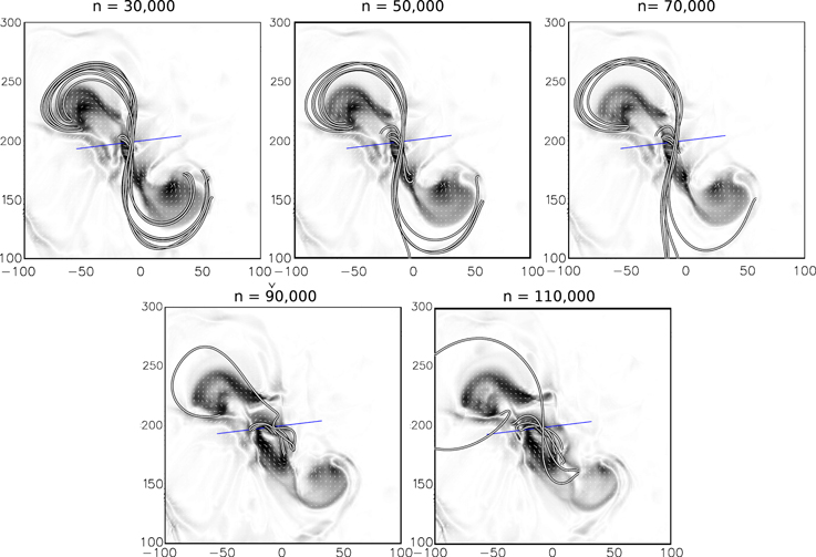
Figure 7. Evolution of field line connectivities for SOl2012-05-08. The field lines are shown on the background of the current density at height of 5 Mm. The maximum value of the current density shown on all panels is fixed at 10,000. The field lines are traced from the same 3D positions in a cross section at the location of the line while the iteration number of the model is changing, i.e., different stages in the relaxation process. It is clear that in the beginning these field lines comprise a flux rope (with about one turn), and as the relaxation proceeds the flux rope rises and gives place to flare field lines resulting in the reconnection at the HFT.
Download figure:
Standard image High-resolution imageIn S12 we showed for the first time that marginally stable NLFFF models can be used to represent the erupting configurations. Then, in Paper I, we used marginally stable and unstable models to derive the QSLs and matched them to the ribbons at the first instance when the ribbons appear in full length. Kliem et al. (2013) showed that when such unstable models, obtained with the flux-rope insertion method, are used as initial conditions to MHD simulations, these flux ropes do erupt in the MHD sense. Further, the evolution of the currents and connectivities in the MHD case is very similar to what the MF process produces. This gives us confidence that the important aspects of the magnetic topology changes can be captured in our magnetofrictional code. Since we do not have explicit time in our iterative process, we can use the QSLs from the different iterations to match the spreading ribbons. In this sense, knowing the time of the image, which has been shown to correspond to a give iteration number by comparing the ribbon and QSL positions, we can get a sense of time. However, the time interval taken from the image do not map linearly to the interval in iteration number. The difference can be explained by noting that the reconnection (diffusion) in the MF evolution does not necessarily proceed with constant or uniformly changing speed, which is the case for the observed ribbon motion as well. Moreover, these speeds are different in the three different cases.
The MF evolution allows for this change in the connectivity. We observe a transfer of flux from connectivity domains but that may not be due to localized reconnection (e.g., at HFT) but rather global diffusion along all the relatively larger non force-free regions. However, there is a strong similarity between what we see in the the evolution of the field connectivity and the MHD simulation of Kliem et al. (2013), which showed that reconnection does indeed happen at the HFT under the flux rope. Thus, we will use the term "reconnection" in the MF simulation, although this process is not yet quantified or understood in the MF sense. Hence, the observed evolution of the flux rope in the models is a result both of the magnetic diffusion scheme that we employ and/or the reconnection under the flux rope that happens during the iterative procedure. In response to the "reconnection" and/or diffusion of the flux rope the output magnetic free energy changes with the iteration number. As shown in Figure 8 the free energy slowly decreases with iteration number. This is logical since free energy is released in the reconnection process, which takes two-J-shaped field lines into the S-shape flux rope and post-reconnection field lines.

Figure 8. Evolution of the magnetic free energy (defined as the difference between the total NLFFF energy and the energy of the potential field) in the process of magnetofrictional evolution for the three sigmoidal regions studies here. The change in free energy and helicity is in response to the diffusion and reconnection of the flux rope.
Download figure:
Standard image High-resolution image3.3. Topological Analysis
The QSL calculation is performed in the same manner as described in Paper I. We use the iterative adaptive mesh method of Aulanier et al. (2005) and Pariat & Démoulin (2012), also used in S12. The squashing factor, Q, is computed for each saved iteration by consecutively doubling the resolution seven or eight times to obtain a single QSL map. Maps of the QSLs for the 30,000th iteration of the unstable models used here are shown in the left column of Figure 9. In the figure Q is highest in the red regions and lowest in the blue. In the right column we display all QSLs above Q = 106 for several different iterations, overlaid on one another and colored by the iteration number. At this stage, it is obvious that the main QSLs in the middle of the domain separate and move away from the PIL as the flux rope rises. The color scale in the panel in the right column is chosen so that the QSLs for the three different iterations have colors spaced by 120° on the color wheel and appear in emission on the black background. In this case the places where the QSLs from the three iterations overlap completely, i.e., where they do not move with respect to each other, appear in white because of the overlap of the three colors. Notice that the QSLs are white far away from the flux ropes in the more potential areas. Since the potential field also has high-Q areas it is useful to look at the movement of the QSLs in erupting motions for additional diagnostics of which QSLs are the "important" ones.
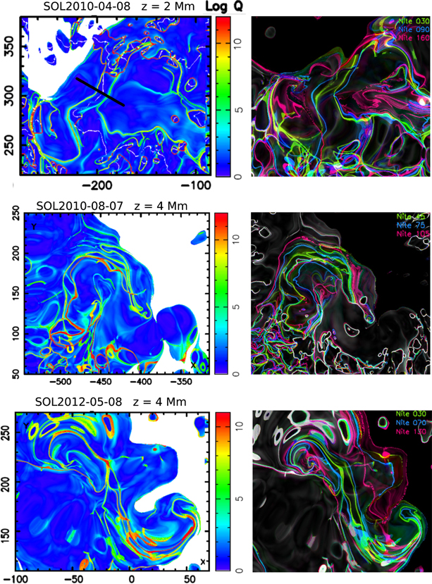
Figure 9. QSL maps for the three regions (left) in  and evolution of the QSLs with iteration for the QSLs with Q-values larger than 106. The different colors represent the different iterations and the iteration number is marked on the plots. The black line in the top left panel shows the location of the QSL cross sections presented in Figure 10.
Download figure:
Standard image High-resolution imageIn Paper I, we matched the QSLs shown in Figure 9 and similar QSLs for another four regions with similar characteristics to the appearance of the ribbons at the first moment when they appear in full length. All matches were very good in the straight part of the ribbons that are parallel to the PIL. In six of the seven cases at least one hook was very well matched, and in some cases both hooks were well represented. We need to note that matching the hooks of the QSLs to the hooks in the ribbons and the associated dimmings is relatively hard since this requires exact knowledge of the footprints of the flux rope. As mentioned in Paper I, the flux-rope path is guided by an observed dark filament in AIA 304 Å, but the endpoints of the filament are not always distinguished well. In addition, the flux-rope footprints may not coincide with the endpoints of the filament.
4. SUPPORTING RESULTS
In this section we prepare the floor for introducing the main results in the next section. Here we explain different features of the MF models and their evolution that allows the easier interpretation of the main results given in Section 5. These include the evolution of the QSL cross-section of the flux rope, which show the rising behavior of the flux rope; the current distributions in one of the region at different locations, which helps to interpret the topology analysis, and the fact that the dimmings are surrounded by QSLs, which is suggested in the standard 3D flare model.
4.1. QSL Analysis of the Expanding Flux Rope
As the iteration progresses, the flux ropes elevate and expand. This behavior can be seen from the QSL cross sections for several different iterations of the SOL2010-04-08 flux rope in Figure 10. The self-crossing of the flux-rope-binding QSL is visible under the flux rope at the HFT. As reconnection proceeds in the magnetofrictional process, the flux rope expands as the iterations continue. At the same time the HFT under the flux rope rises and the legs of the HFT spread. The footprints of the HFT are the QSLs shown in Figure 9, which move away from the PIL as the iteration process progresses. In this case the HFT rises from 8 to 90 Mm in height, and the legs spread from 10 to 40 Mm in a cross section, which is chosen to be approximately parallel to the flux rope in the middle of the active region.
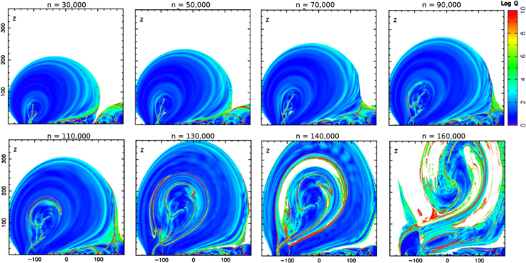
Figure 10. Q cross sections for the SOL2010-04-08 region. The cross sections are taken at the location of the black line in the top left panel of Figure 9. The iteration number is marked on the plots. Notice the well-defined HFT (red QSLs) and its progressive elevation with iteration number (time), which corresponds to what is expected from the standard model.
Download figure:
Standard image High-resolution imageIn addition to the elevation of the HFT, the flux rope expands significantly, occupying a larger and larger volume. In the process of expansion, other QSL structures appear within the flux rope, but the overlaying arcade remains free of complicated and strong QSLs. Therefore, we can be sure that the location where reconnection takes place is primarily at the HFT (if not along the whole QSL), under the flux rope. In Figure 10 one can also notice that the flux rope is inclined to the side. This is because the northeastern polarity is stronger than the opposite polarity, creating a more magnetic pressure gradient that pushes the flux rope to one side. The direction of inclination also matches the direction of the early-time CME propagation, which is deflected toward the equator and to the east (see STEREO movies in the online material of Su et al. 2011). The result that this flux rope is inclined is most probably a property of many flux-rope configurations on the sun because in most cases both polarities are not perfectly balanced and the magnetic flux is not distributed smoothly in the same way. Thus, these modeled configurations can present suitable conditions for the study of asymmetric reconnection in which the current density is not the same across the reconnection current sheet.
From the time stamp of the images and the iteration number we show that the QSLs have spread over 100,000 iterations, which corresponds to 26 m 36 s of the real time of ribbon evolution. From this timescale and the change in position of the HFT as seen in Figure 10, the HFT has gone up with ∼82 Mm in 130,000 iterations, or 34 m 58 s, which gives an average speed of the reconnection site upward motion of 40 km s−1. In the same figure, the top of the flux rope goes up with 308 Mm in the same period of time, which gives a velocity of 147 km s−1. This motion consequently produces the CME, which was measured in the corona just below the occulting disk of STEREO to be 150 km s−1 (Kliem et al. 2013). Similar analysis can be done for all studied regions. This demonstrates the close correspondence between observations and the evolution of the unstable flux rope in the MF process.
4.2. Current Distributions and the Structure of Flux Ropes
As shown in S12 and Paper I, there are the main current concentrations that overlay the prominent QSLs that bind the flux rope from the overlaying arcade. These relatively thin (at the level of the grid resolution) current sheets can be seen in Figure 11, which shows four different current-density cross sections through the flux rope in the SOL2010-08-07 region in the 90,000th iteration of the magnetofrictional evolution. A horizontal cut of current density is shown in the top panel. The flux-rope path is shown with a yellow line and the locations of the vertical cuts are shown with blue lines. From this picture it is clear that not only is there an HFT under the flux rope, but it extends over most of the length of the flux rope. In this case the flux rope is also slanted to one side, which matches the direction of lift-off of the filament eruption seen in this region. It is also clear that the height of the HFT is different along the flux rope. The HFT is lowest in the southwestern part of the region close to the sunspot, where the right footprint of the flux rope is located. This is probably caused by the strong fields emanating from the sunspot, which are successful at pushing the flux rope down.

Figure 11. Horizontal map of the current density at a height of 5100 km (top panel) for the SOL2010-08-07 sigmoid, iteration 90,000. The positions of the four vertical cross sections are marked with blue lines. Cross sections at the locations of the blue lines are shown in the panels below. The current density maximum is fixed at 20,000 G Mm−1 for all panels. Notice the well-defined HFT at all these location. The HFT is at the largest height (at about 35 Mm) at the location of the westernmost cross section.
Download figure:
Standard image High-resolution imageIt is useful to note that the HFT in the case of our unstable models always displays an X-like cross section, while in the MHD simulations of (Janvier et al. 2013, Figure 1) and (Kliem et al. 2013, Figure 12), the HFT turns into an elongated current sheet as the flux ropes rises. This might be due to the fact that reconnection happens more readily in the MF code than in the MHD code, so the current sheet dissipates before it has a chance to grow in length.
4.3. Transient Coronal Holes and QSLs
In addition to the flare ribbons, we can match features related to the CME evolution. As described in the standard model, as the flux rope erupts it carries coronal plasma with it, which reduces the plasma density at the footprints of the flux rope in the corona. Hence, in the vicinity of the flux-rope footprints there is reduced emission (emission depends on the square of the density), which is observed in the AIA 193 and 211 Å channels as transient CHs. An image of these transient CHs at the moment when they first appear in the 193 Å channel is shown in the background of Figure 12. The blue lines are the QSLs taken from the 130,000th iteration. It is obvious that the hooks of the QSLs outline the transient CHs capturing their elongation in the north–south direction. The centers of the QSL hooks are located at (−240, 270) and (−120, 330), with the first being close to the center of the eastern dimming. The eastern CH is better matched by the encircling QSL and the western one has a more complicated shape. It also seems to lie to the south of the QSL hook, which is an indication that the western flux-rope footprint is not well-constrained or there was considerable slippage of the flux-rope leg that cannot be accounted in the MF simulations. This configuration of QSL hooks and flux-rope footprints has been predicted by Janvier et al. (2013).

Figure 12. QSL map for the 130,000 iteration of the SOL2010-04-08 region overlaid on an images of the flare ribbons and dimmings in AIA 193 Å for the time shown on the figure. Notice that the eastern dimming is very well matched by the corresponding QSL hook. The western one does not show such a good match probably because that footprint of the flux rope is not well constrained.
Download figure:
Standard image High-resolution imageAs determined in the standard 3D model, the hooks of the QSLs should circle around the two footprints of the flux rope and should do so more tightly for larger poloidal flux in the flux rope. For larger poloidal flux the hooks should also cover a larger area since there is overall more flux in the flux rope. The effect of the poloidal (and axial) flux on the shape of the QSL hooks will be studied in detail in a future parameter study, as mentioned in Paper I. Since the initial poloidal flux in this region is only 5 × 10¹⁰ Mx cm−1 (See Table 1), and the final poloidal flux is even less due to the diffusion process, these QSL hooks are not very tight, which matches the large size of the transient CHs as compared to the initial flux-rope footprints.
The other two regions show dimmings that do not match the QSLs hooks because the dimming is situated farther away from the inserted flux-rope footprints. In the case of SOL2012-05-08, only the southern dimming is visible and our flux-rope path is not constrained well there as explained in the discussion section (see the online movie). SOL2010-08-07 also shows only one clear dimming much to the south of the flux-rope footprint in the sunspot, maybe due to slippage of the flux-rope leg in that part of the region (see the online movie).
5. MAIN RESULTS
5.1. Ribbons and QSL Time Evolution
Here, we overlay the QSLs at low heights for several different iterations with images of the flare ribbons taken at different times that show the transverse motion of the ribbons. The QSLs are extracted in a similar manner to Paper I, i.e., only QSLs above a certain threshold in Q and in the current density, j, are shown in the overlays. By selecting the QSLs to be situated in regions of large current density, we ensure that we are picking the QSLs related to current build-up and non-potentiality, where reconnection can take place and power a flare.
The maps chosen for the overlays are at the same height as the ones discussed in Paper I and have been projected onto a sphere with radius a corresponding to the given height of the original Cartesian maps. The offsets between the QSL maps derived from the magnetic field distributions before the flares have been adjusted with the time difference between tmag and the times of the ribbon images (tribbon). We apply an additional small offset that is determined in Paper I based on the co-alignment of various particular features in the magnetic flux distribution that remain the same between tmag and tribbon. The average error in the alignment is 3''–6''. Now, we consider each of these overlays for the three regions studied here and discuss the quality of the match.
- 1.SOl2010-04-08. For the flare evolution in SOL2010-04-08, we show overlays for six different iterations of the unstable model in Figure 13. The QSLs are shown in blue and the AIA 304 Å images are shown in red in the background. The best match, as in Paper I, is the central part of the flare ribbons that are parallel to the PIL between x and y positions (−295:−235) and (420:470), respectively. There is some structure in the western QSL hook that matches the emission in 304 Å. However, as in the first match shown in Paper I, the eastern hook does not match very well, i.e., the QSL hook seems to be broader than the ribbon hook. The ribbons, as can be seen from the images, mostly move in their central part where they are parallel to the PIL and this motion is very well captured by the different iterations. The ribbons/QSLs in their central part spread by 20 Mm in 26 m 40 s, which gives an average velocity in the center of the ribbons at (x, y) = (−250, 440) of 12.5 km s−1. In this case, 26 m 40 s corresponds to 100,000 iterations, so the timescale can be derived to be on average 16 s per 1000 iterations. To compute this number we have taken only the first and the last iteration that correspond to the whole interval of ribbon evolution shown in Figure 13. However, the timescale derived from two consecutive iterations from the figure give slightly different results due to the reasons pointed out in Section 3.2.
- 2.SOL2010-08-07. The evolution of the QSLs and ribbons is shown in Figure 14 for this region. The first iteration matches the first instance of the flare ribbons as can be seen from the figure in Paper I. At the 60,000th iteration, i.e., at 18:09 UT, the northern flare ribbon is still experiencing a zipper motion and is expanding to the east. It has reached only approximate position (x, y) = (−540, 180) in this snapshot. After the conclusion of the zipper motion, the northern hook does not move too much in the direction perpendicular to the PIL. This is probably because the northern polarity is stronger. The perpendicular motion of both ribbons should sweep roughly the same magnetic flux in both polarities, which means that if the flux is stronger in one polarity the corresponding ribbon should move slower, which is what we observe here. This effect has been predicted by the theory, but here we are able to model it for the first time. The northern ribbon has almost fully extended in the image corresponding to the 75,000th iteration and the match to the ribbons has improved. The match is very precise at the 90,000th iteration where both ribbons are very well reproduced by the QSLs. In the last two images showing the ribbons in 304 Å, we see a very good match to the northern ribbon. The southern QSL misses part of the southern ribbon, which has stopped moving in its eastern part, but still the location of the QSL approximately matches the location the ribbon. Overall this region represents a very good match between the motion of the QSLs and the ribbons. The ribbons spread by 45 Mm in 36 m 08 s, which corresponds to 55,000 iterations. This gives an average spreading velocity at (−550'', 175'') of 20.75 km s−1. These ribbons move at the largest velocity of all ribbons studied here, which might be because this is the largest flare, an M-class flare. In order to power such a large flare more flux needs to be converted in the reconnection processes, which can be gathered over larger areas covered by the ribbons in a given time interval.
- 3.SOL2012-05-08. This is the most challenging active region to model since the flux-rope path could not be constrained well by the pre-flare configuration as discussed in Section 3.1. As explained in Section 2.3 and in the discussion section, the flux rope either changes connectivity in the process of eruption or previously invisible parts of it become apparent when the first flare ribbons start to appear. As discussed in Section 3.1 we modeled this region with three different paths. However, we got meaningful results only from the path that follows the S-shaped filament visible over a long time before the eruption.In this region the straight parallel parts of the ribbons are very well matched in all four panels of Figure 15. The hooks experience very little motion as in the case of SOL2010-04-08. In this case the parallel parts of the ribbons spread by 15 Mm in 17 minutes or 80,000 iterations. This gives an average velocity of motion perpendicular to the PIL of 14.7 km s−1. As can be seen from comparing these numbers for the three regions, the ribbons move at different speeds perpendicular to the PIL, with this region being the slowest. This is probably dependent on the reconnection efficiency, the interplay between reconnection and torus instability, which pulls the flux rope up, and the strength of the polarities.
Figure 13. QSL maps overlaid on six different images of the flare ribbons in the SOL2010-04-08 sigmoid. The images are taken at four consecutive times showing the progression of the ribbons in the region. The QSL maps are taken at four different moments in the iteration procedure—spaced by 20,000 iterations. The current is in normalized units, where the maximum of the current is 1. Notice that the QSLs move in the same manner as the flare ribbons, which is most obvious in the straight middle part of the ribbons.
(An animation of this figure is available.)
Download figure:
Video Standard image High-resolution imageFigure 14. QSL maps overlaid on six different images of the flare ribbons in the SOL2010-08-07 sigmoid. The images are taken at four consecutive times showing the progression of the ribbons in the region. The QSL maps are taken at four different iterations—spaced by 15,000 iterations. The current is in normalized units, where the maximum of the current is 1. Notice that the QSLs move in the same manner as the flare ribbons, which is most obvious in the southern flare ribbon.
(An animation of this figure is available.)
Download figure:
Video Standard image High-resolution imageFigure 15. QSL maps overlaid on four different images of the flare ribbons in the SOL2012-05-08 sigmoid. The images are taken at four consecutive times showing the progression of the ribbons in the region. The QSL maps are taken at four different iterations—spaced by 20,000 (40,000 for the last image) iterations. The current is in normalized units, where the maximum of the current is 1. Notice that the QSLs approximate the motion of the flare ribbons.
(An animation of this figure is available.)
Download figure:
Video Standard image High-resolution imageThis motion of the QSLs in conjunction with the flare ribbons is shown here for the first time. We have shown the dynamic nature of the QSLs, which is to be expected since the reconnection site rises in the corona so that more and more volume is contained in the post-reconnection field lines laying in the domain under the flux rope and bound by the QSLs. To our knowledge, topological features have been regarded as stationary and the flare features have sometimes been considered to pass over them (e.g., Chen et al. 2011). This is certainly true for the positions of reconnecting field lines, the footpoints of which have been shown to move along the QSLs in the photosphere (Aulanier et al. 2012).
The fact that magnetic field models constrained only by pre-flare observations can reproduce the change in topology associated with flares with unprecedented success, leads us to believe that this method and analysis has predictive capabilities. We have shown that it is possible to predict the evolution of the flare features very well knowing only the pre-flare configuration of the active region. This is the first result of this kind that has been ever shown.
5.2. Flare Loops and HFTs
In S12 we demonstrated the presence of different connectivity domains in cross section through the flux rope, which can be seen in Figures 10 and 11. One can clearly see the four-way separation of the domain represented by the X-like HFT in both of these figures. According to the standard flare picture shown in Figure 1, the flare loops should lie under the HFT in the volume bound by the flux-rope QSLs. We now verify that this is the case. In Figure 16 we show some reconnected field lines traced from the 75,000th iteration of the unstable model in SOL2010-08-07, which have been overlaid on a 171 Å image of flare loops. The match is qualitatively very good both in the northeastern and southwestern part of the region. The footpoints of the loops are also matched well as we displaythe amount of shear in them. The loops in the upper part of the region are less sheared than the loops that have one of their footpoints in the sunspot. The loops in the upper part of the region are shown in the third row of the figure in horizontal cut at 5 Mm above the photosphere (Figure 16, left column) and in vertical cross section through the flux rope at the location of the blue line (right column, panel corresponding to cross-section 1). The loops in the lower part of the region are shown in the corresponding panels in the fourth row. From these panels it can be seen that the shear is larger where the HFT is situated at a lower height, which is explained with the fact that the loops are closer to the HFT and still carry significant shear from the pre-flare flux-rope field lines. At a later time loops farther away from the HFT dominate the emission, which have a more potential shape.
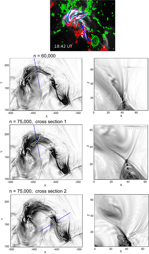
Figure 16. Top: A 171 Å AIA image taken at 18:42 UT with overlaid flare loops. These field lines have been taken from the 105,000th iteration model. The magnetic flux distribution is shown with red (positive) and green (negative) contours. The same field lines are shown overlaid on the current distribution at a height of 5 Mm (left column) and in cross sections of the current through the middle of the bundles (right column). The maximum of the current density in all panels is fixed at 60,000 G Mm−1. All of these field lines lie under the HFT as is expected for post-flare loops for all three cases. The second row shows field lines in the same cross section for the 90,000th iteration and the third and fourth rows show the field lines in the 105,000 iteration. It is clear that the field lines are more sheared in the earlier iteration when the HFT lies at a lower height.
Download figure:
Standard image High-resolution imageAulanier et al. (2012) suggest that the field lines transition to a lower shear stage, i.e., they experience the strong-to-weak shear transition as time progresses, which they reproduce with their MHD simulation. This change in shear has been observed multiple times in flares (e.g., Su et al. 2006; Aulanier et al. 2012), which serves as the basis of the standard model in three dimensions. This shear transition is a very common behavior in two-ribbon flares (Su et al. 2007), which can be seen in the online animations of the three regions. To confirm this, we show in the second row of Figure 16 field lines traced from under the HFT in the cross section shown in right panel. These plots are taken 15,000 iterations earlier than the loops/field lines in the top panel. It can be seen that the shear is larger in the 60,000th iteration case than in the 75,000th one by a small but noticeable amount.
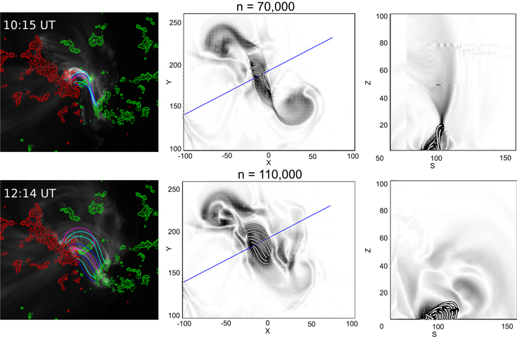
To further explore the strong-to-weak shear transition, we show field lines from two different iterations of the SOL2012-05-08 flux rope in Figure 17. These are overlaid on 171 Å images of the loops separated by 119 minutes and 40,000 iterations. It can be gleaned from all plots in the first and second row that the shear decreases with time, with the loops in the second row being significantly more potential than the ones in the first row. The loops in the first cross section are even slightly twisted and are lying directly under the HFT. In the second row, the HFT has already disappeared since the flux rope has fully erupted, so the remaining loops are almost completely potential.
Figure 17. Left column: flare loops in SOL2012-05-08 for two different times. The iteration number of the models from which we have taken these field lines is marked on the corresponding plots. The magnetic flux distribution is shown with red (positive) and green (negative) contours. The same field lines are shown on a plot of the current density in horizontal cut at z = 5000 Mm (middle column) and in cross sections of the current through the middle of the bundles (right column). The maximum of the current density in all panels is fixed at 10,000. The strong-to-weak shear transition is evident in these plots.
Download figure:
Standard image High-resolution image
The level of initial shear, according to the standard 3D model of Aulanier et al. (2012) depends on the amount of shear in the pre-eruption flux rope, which gets transfered to the first reconnected field lines. As time progresses, these field lines relax and their tops move away from the reconnection site, thus changing their shear. In this process their footpoints also separate, which is reflected in the spreading motion of the flare ribbons. There are almost no loops rooted in the hooks at that time since they have already slipped and changed their connectivities in the relaxation process (see the animations of their slipping motion in the online material of Janvier et al. 2013).
Being able to match the initial appearance and the strong-to-weak shear transition in the flare loops with post-reconnection field lines from the models in several cases speaks further to the predictability of the method. Kliem et al. (2013) already showed that our unstable models evolve through these stages in the MHD sense, but here for the first time we show that an MF simulation is sufficient to look at the evolution of several flare features. And since data-constrained and even data-driven MF simulations (e.g., Gibb et al. 2014) are much faster than data-constrained and the non-existent data-driven MHD simulations, the use of the former is likely to be more efficient in operation space weather predictions.
6. CONCLUSIONS
In this paper we showed the first comprehensive topological study of data-constrained magnetofrictional simulations of a selection of flaring sigmoidal active regions that display flare ribbons, transient coronal holes, and flare loops during the time of major solar flares. We put these observed features in a topological context, utilizing QSL maps obtained from data-constrained unstable magnetic models. Schrijver et al. (2011) and Aulanier et al. (2012) have classified the observed flare features using idealized MHD simulations to obtain the topology analysis. We have extended these archetypal simulations to real solar active region configurations. We show an excellent match between QSL maps taken at low heights in the corona and chromosphere and the locations and extent of flare ribbons at different times during the progression of the flare. We also show that the main flux-rope-binding QSLs evolve in time together with the spreading flare ribbons—a novel result. Based on this analysis we have computed the average separation speed of the QSLs in all three cases and related the speed to the strength of the flare and the magnetic flux distributions. In addition, we derived the average timescale of the magnetofrictional evolution, i.e., the total number of iterations corresponding to the total period of time of observed flare ribbon evolution. We also discussed the fact that this timescale varies with iteration since the evolution of the configuration does not proceed with the same speed.
From the QSL cross sections through the flux rope, we can measure the rate of elevation of the HFT in the unstable models as well as the expansion speed of the flux rope. In the case of SOL2010-04-08, we get a speed of the expanding flux rope that closely approximates the one derived from observations of the propagating CME in the corona by Kliem et al. (2013). Finally, we showed that the hooks of the QSLs also surround the transient coronal holes as predicted by the standard 3D model of Janvier et al. (2013).
In this model, as shown by Aulanier et al. (2012), the flare field lines, corresponding to the flare arcade, experience a strong-to-weak shear transition. The amount of post-reconnection shear depends on the the amount of pre-flare shear contained in the two-J-shaped field lines, which, as shown in S12, go through tether-cutting kind of reconnection to produce the field lines lying in the domain under the HFT. We have demonstrated that 3D data-constrained modeling produces the right shape and shear for the reconnected field lines when compared to observed flare loops in AIA. We have shown that the amount of shear in these field lines varies both with location and time (iteration number).
In one case we also showed that the flux-rope cross sections are not symmetric, but are slanted to one side in response to the uneven distribution of the ambient magnetic flux. This analysis has potentially very strong implications for the study of 3D reconnection in realistic coronal magnetic fields, which lack the usual symmetry that many reconnection simulations and laboratory experiments employ. The above analysis serves to confirm the standard 3D picture with observations and data-constrained modeling for the first time.
Our models show that the QSLs separate and the separation matches the ribbon spreading. While this is theoretically predicted by theory and has been shown that QSLs indeed are being displaced perpendicularly along the eruption (Janvier et al. 2013), here for the first time we show it in a data-constrained model. This is a new very strong proof of the standard model. We demonstrate for the first time that energy flowing from the reconnection site is flowing down along the flux-rope QSL and match it with the dynamic position of the ribbons during the whole development of the flare. It is still widely believed that QSLs are static and that they do not move during the eruption. This clearly shows that it is not the case and that the time-dependent position of the ribbons are "always" matching with the time-dependent position of the QSLs (hence the reconnection site) during this separation phase. We are able to reproduce the differential displacement of the ribbons. i.e., ribbons move more where the field is weak than where the field is strong because of the reconnection rate being linked with the amount of magnetic flux processed. This analysis shows a very strong predictive capability. Technically, we should be able, using marginally unstable NLFFF models, to predict the displacement of the ribbons in a flare.
Hinode is a Japanese mission developed, launched, and operated by ISAS/JAXA in partnership with NAOJ, NASA, and STFC (UK). Additional operational support is provided by ESA, NSC (Norway). This work was supported by NASA contract NNM07AB07C to SAO. The QSL computations have been performed on the multi-processors TRU64 computer of the LESIA. A.S. is supported by the NASA LWS Jack Eddy postdoctoral fellowship. Y.S. is supported by NSFC # 11333009 and Youth Fund of Jiang Su # BK20141043. We would like to thank the AIA team for supplying the data for this study.