


ABSTRACT
Neutron monitors (NMs) are ground-based detectors of cosmic-ray showers that are widely used for high-precision monitoring of changes in the Galactic cosmic-ray (GCR) flux due to solar storms and solar wind variations. In the present work, we show that a single neutron monitor station can also monitor short-term changes in the GCR spectrum, avoiding the systematic uncertainties in comparing data from different stations, by means of NM time-delay histograms. Using data for 2007–2014 from the Princess Sirindhorn Neutron Monitor, a station at Doi Inthanon, Thailand, with the world's highest vertical geomagnetic cutoff rigidity of 16.8 GV, we have developed an analysis of time-delay histograms that removes the chance coincidences that can dominate conventional measures of multiplicity. We infer the "leader fraction" L of neutron counts that do not follow a previous neutron count in the same counter from the same atmospheric secondary, which is inversely related to the actual multiplicity and increases for increasing GCR spectral index. After correction for atmospheric pressure and water vapor, we find that L indicates substantial short-term GCR spectral hardening during some but not all Forbush decreases in GCR flux due to solar storms. Such spectral data from Doi Inthanon provide information about cosmic-ray energies beyond the Earth's maximum geomagnetic cutoff, extending the reach of the worldwide NM network and opening a new avenue in the study of short-term GCR decreases.
Export citation and abstract BibTeX RIS
1. INTRODUCTION
Neutron monitors (NMs) are ground-based detectors of secondary neutrons in atmospheric showers from cosmic-ray ions. Initially designed by Simpson (1948), NMs have been used for precise monitoring of time variations in the cosmic-ray flux, and some routinely achieve 0.1% accuracy in hourly rates. The look direction of the detector sweeps through space along with Earth's rotation, so daily (diurnal) variations in the NM count rate provide additional information on the directional distribution and anisotropy of cosmic rays (e.g., Bieber & Chen 1991; Okazaki et al. 2008; Yeeram et al. 2014). Time variations in the cosmic-ray density and anisotropy provide important information about solar energetic particles from solar storms (e.g., Meyer et al. 1956; Bieber et al. 2013) and effects on the Galactic cosmic-ray (GCR) distribution due to coronal mass ejections or their associated shocks (known as Forbush decreases; Forbush 1937; Cane 2000), solar wind structures that corotate with the Sun (Simpson 1954; Elliot 1960), and the solar activity cycle (known as solar modulation; Forbush 1954; Moraal et al. 1989).
Cosmic-ray showers in Earth's atmosphere produce many secondary particles, so a large ground-based detector can measure high count rates very precisely. The disadvantage is that the energies of primary cosmic rays are not directly detected. Fortunately, the Earth provides a natural magnetic spectrometer, so a primary particle must have a rigidity  where p is momentum and q is charge, that exceeds the geomagnetic cutoff for a given epoch, location, and arrival direction. The vertical geomagnetic cutoff varies from ∼17 GV in and near Thailand down to
  GV in polar regions, where the primary ion energy must exceed an atmospheric cutoff corresponding to
  GV to be detectable at ground level. Atmospheric neutrons are predominantly produced by cosmic-ray ions just above the cutoff rigidity, so the worldwide NM network provides some spectral information from a comparison of NM count rates at varying cutoff rigidity. Such a comparison may be facilitated by the use of a portable intercalibration NMs (Moraal et al. 2000; Krüger et al. 2008; Aiemsa-ad et al. 2015). In contrast, atmospheric muons predominantly result from cosmic rays of much higher rigidity, and surface muon detectors are sensitive to a median rigidity that varies from ∼60 to ∼110 GV, depending on the selected direction of incidence (Okazaki et al. 2008).
There are difficulties in tracking short-term cosmic-ray spectral variations by comparing count rates from two NMs at different locations. As an example, let us consider data from the recently installed Princess Sirindhorn Neutron Monitor (PSNM; Figure 1) at Doi Inthanon, Thailand, and from the Yangbajing Neutron Monitor in Tibet, China. In the worldwide NM network, Doi Inthanon has the highest vertical cutoff rigidity (16.8 GV) and Yangbajing has the second highest (about 13.8 GV during the time of interest). The Yangbajing/Doi Inthanon count-rate ratio (Figure 2) might be expected to relate to the cosmic-ray spectral index with a higher ratio for a higher spectral index (softer spectrum). Over a yearly timescale, the result is as expected, with the well-known effect of a softer spectrum during the GCR maximum (in late 2009) near the time of sunspot minimum (late 2008). However, over shorter timescales, the ratio varies more erratically and does not match previous findings of spectral hardening during short-term cosmic-ray decreases (e.g., Cane 2000; Gil & Alania 2010).9 Therefore, it does not seem to accurately indicate subannual spectral variations. Our interpretation is that while NM data often have statistical accuracy better than 0.1% in hourly rates and 0.02% in daily rates (as is the case for the mountain-top stations of Yangbajing and Doi Inthanon, which record particularly high count rates), they also involve some unknown systematic effects, probably related to local atmospheric conditions (other than barometric pressure, which has already been corrected for) or sampling particles from a different set of asymptotic directions in space, which make it difficult to determine subannual spectral variations by comparing data from two stations. This motivates an attempt to determine spectral variations from single-station data, using a fraction or ratio in which some systematic errors may cancel out.

Figure 1. (a) Princess Sirindhorn Neutron Monitor station at the summit of Doi Inthanon, Thailand's highest mountain (at 2560 m altitude). (b) View inside the station, showing the 18-tube NM (right) and three bare counters (center). (c) Components of the NM (to scale). Pb: Lead producer "rings with wings," in which a cosmic-ray-generated atmospheric secondary particle, typically a neutron of 10 MeV to 10 GeV, can disrupt a lead nucleus to produce several low-energy neutrons. PE: Polyethylene, through which high-energy neutrons typically pass without interacting, but low-energy neutrons are efficiently moderated toward the thermal energy range. The 3 inch PE reflector surrounding the monitor serves to block low-energy neutrons from the environment while trapping most neutrons produced by interactions in the lead. PC: 10BF3 gas proportional counter tube (viewed in cross section) in which neutrons (especially those at low energy) interact with 10B and the reaction products produce a strong, characteristic electronic signal. Wood: Wooden supports for the lead rings.
Download figure:
Standard image High-resolution image
Figure 2. Comparison of daily count rates from 2007 December to 2011 February from the Yangbajing and Doi Inthanon NMs at vertical cutoff rigidities of about 13.8 and 16.8 GV, respectively, along with the count-rate ratio. Each NM count rate has precise statistical accuracy (better than 0.02%). Variations in the count-rate ratio might be expected to indicate changes in the cosmic-ray spectrum. While the long-term rise and fall in the ratio are consistent with the known spectral softening near sunspot minimum (GCR maximum), shorter-term variations seem to have a systematic uncertainty and do not clearly indicate the known spectral hardening during short-term decreases. In the present work, we develop a method to study short-term spectral variations using a single NM, without the systematic uncertainty of a station-to-station comparison.
Download figure:
Standard image High-resolution imageIt has long been recognized that a single NM station also has the potential to track variations in the atmospheric secondary particle spectrum, which in turn may reflect the rigidity spectrum of GCRs. The multiplicity, typically defined as the number of neutrons registered by a single counter tube within a specific time period, has previously been proposed as an indicator of the cosmic-ray spectrum. The idea is that more energetic atmospheric neutrons can cause a lead nucleus in the producer to eject a larger number of neutrons, resulting in a higher multiplicity (Hatton 1971). If we use M1 to indicate the rate of multiplicity 1 events, M2 for multiplicity 2 events, and so on, previous work has typically examined either a mean multiplicity  or ratios such as M1/M2, in which case a lower value is taken to indicate a harder spectrum. However, we sometimes find an increasing M1/M2 during Forbush decreases, which again does not match the common observation of spectral hardening during spectral decreases.
Recent work has examined neutron time-delay histograms from NM counter tubes (Bieber et al. 2004, 2005; Balabin et al. 2008; Kollár et al. 2011; Balabin 2013), as recorded by specially designed readout electronics at some NMs. Here the time delay refers to the time interval between successive neutron detections in one counter. Bieber et al. (2004) indicated that time delays over ∼4 ms are dominated by chance coincidences, with an exponential distribution characteristic of unrelated events, while shorter time delays are mostly due to the correlated arrival of neutrons from the same nuclear interaction, typically an interaction in the lead producer. Bieber et al. (2005) showed that during the giant relativistic solar-particle event of 2005 January 20, the exponential distribution changed to reflect an increased count rate. To our knowledge, such recording systems have not yet been used to study temporal variations in the GCR spectrum.
In the present work, we report observational results from the PSNM at Doi Inthanon, where in addition to a standard 18-tube NM with a count-rate readout to monitor the GCR density and anisotropy, we have deployed two independent systems to study secondary particle spectral variations: (1) specialized electronics to record neutron time-delay histograms (Bieber et al. 2004) and (2) "bare" neutron counters with a moderator but no lead producer or reflector (Stoker 1985), as previously used with the South Pole NM to study spectral variations of relativistic solar ions (Bieber & Evenson 1991; Bieber et al. 2002, 2013; Ruffolo et al. 2006). We show that standard measures of multiplicity can be dominated by chance coincidences. We have developed techniques for analyzing time-delay histograms to remove the effect of chance coincidences and measure the "leader fraction" L of neutrons that did not follow a previous neutron count in the same detector due to the same atmospheric secondary particle. Both L and the bare/NM ratio exhibit an annual wave, presumably due to atmospheric effects or (in the case of bare/NM) effects related to accumulation of rainwater at ground level. After correcting for these, the leader fraction L provides a clear indication of spectral hardening during some Forbush decreases, which is weak or absent during other GCR decreases, providing new information on short-term GCR responses to solar phenomena.
2. PRINCESS SIRINDHORN NEUTRON MONITOR
The PSNM has taken data since 2007 August and has operated in its full 18-tube configuration since 2007 December. It is located at the summit of Doi Inthanon, Thailand's highest mountain, at geographic coordinates 18 59N and 9849E, with a vertical cutoff rigidity of 16.8 GV. It is the first and only full NM in mainland Southeast Asia, and it is the world's first NM station at such a high cutoff.
PSNM is located at an altitude of about 2560 m above sea level. Because cosmic-ray showers are rapidly absorbed in the lower atmosphere, a high altitude greatly enhances the neutron count rate. For example, the count rate of each bare counter at the PSNM station is found to be  times that of a similar bare counter operated at Mahidol University in Bangkok, Thailand, near sea level.
Figure 1(a) shows the PSNM building, which is 10 × 10 m2 in size with a peaked roof to avoid accumulation of rainwater. The PSNM uses the standard NM64 design (Hatton & Carmichael 1964), with 18 BP-28 proportional counter (PC) tubes arranged in a single row to reduce edge effects (Figures 1(b) and (c)). The monitor contains 29 t of lead producer, where an atmospheric secondary particle from a cosmic-ray shower can disrupt a lead nucleus, causing the production of several low-energy neutrons. These can be trapped within the outer polyethylene (PE) reflector (which also serves to exclude most low-energy neutrons from the environment). There is also a cylindrical PE moderator around each PC tube, which can reduce the neutron energy toward the thermal energy range.
The innermost PC tubes contain BF3 gas, enriched to 95% 10B at a pressure of 200 mm Hg (at 20 °C). When neutrons enter the PC with lower energy, they are more likely to induce fission of 10B to produce 7Li and 4He. The product nuclei, with a combined kinetic energy of at least 2.3 MeV, yield a strong signal in the PC with very little background noise. On average, the count rate of a PC in the PSNM is  The two edge tubes have count rates that are
  lower than the 16 middle tubes because the edge tubes have less lead producer in their proximity.
While the detector is called a neutron monitor, that is somewhat misleading because other atmospheric secondary particles can also disrupt a lead nucleus, resulting in the release of neutrons that are detected in the PCs. Monte Carlo simulations of the PSNM (Aiemsa-ad et al. 2015) indicate that 80% of the count rate is due to atmospheric secondary neutrons, predominantly in the energy range of 10 MeV to 10 GeV, while 15% is due to protons, and various other secondary species contribute 5%. In any case, the purpose of a neutron monitor is to measure the flux of cosmic rays impinging on the atmosphere above the detector. For Doi Inthanon, where the vertical cutoff rigidity is 16.8 GV, our calculated response function implies a median primary cosmic-ray rigidity of 35 GV and a 10th to 90th percentile range of 18 to 155 GV. Note that the cutoff itself depends on the direction of incidence and changes with time and geomagnetic conditions.
In addition to the 18-tube NM64 detector (or "18NM"), the PSNM station also has three bare neutron counters (Figure 1(b); see also Figure 2 of Aiemsa-ad et al. 2015). Each bare counter comprises a BP-28 PC surrounded by a standard PE moderator but with no lead producer or PE reflector. The bare counters are sensitive to atmospheric secondary neutrons over a very wide energy range, and the overall count rate is much lower because of the absence of lead producer. The count rate per tube is  which is about six times lower than the count rate per tube in the 18NM.
Because atmospheric secondary particles are rapidly absorbed in the atmosphere, an NM count rate is generally corrected for barometric pressure, which provides a measure of the air mass above the detector (atmospheric depth). PSNM is currently operated with two Digiquartz barometers (from Paroscientific, Inc.) to measure barometric pressure to a precision of 0.01 mm Hg. One measures the air pressure in a storage room at the side of the station, which has openings that allow air to come inside, and the other is connected to a pressure head (from Vaisala) that is designed to minimize the error due to a varying wind angle and is mounted above ground and several meters to the side of the building. The two pressure values generally agree to within 0.05 mm Hg, indicating that the two types of pressure measurement give similar results. The PSNM data are corrected with a coefficient of 0.854% mm Hg−1 to a standard pressure of 563 mm Hg. Another serious concern in a humid, tropical environment is the effect of humidity on the electronics. We continuously operate a dehumidifier inside the building and monitor the relative humidity, which should remain below 50% for proper operation of the electronics. We also monitor the temperature in the station and at three locations along each PC tube. We do not control the temperature in the building (which greatly reduces operating costs in comparison with some other NM field stations), and the temperature inside the 18NM has very little variation throughout the year because of the low seasonal temperature variation in the tropical environment and the large thermal mass of the lead. We find no significant variation of the PSNM count rate due to temperature variation, so no temperature correction is applied.
PSNM also employs an electronic data-acquisition system that can record time delays between successive neutron counts at the same tube, based on a system used in a latitude survey (Bieber et al. 2004). PSNM is the first fixed NM station to employ that system. Similar systems have been developed by other groups (e.g., Balabin et al. 2008; Kollár et al. 2011).
For each of 18 NM counter tubes and three bare counter tubes and for each time interval, our system outputs two time-delay histograms over short and long timescales, recording the frequency of time delays in 1023 time bins of width  μs and 1024 bins of nominal width
  μs, respectively, as shown in Figure 3. After a time corresponding to 1024 of the latter bins,
  ms, the time delay overflows, and a count is entered into the histogram according to the remainder.
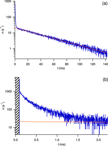
Figure 3. Example of time-delay histograms collected for one neutron counter tube in the PSNM at Doi Inthanon during one hour. (a) Long time delays follow an exponential distribution (red) as expected for unrelated neutron detection events. (b) At short time delays ( ms), the distribution deviates substantially from that exponential because many events are related, coming from the same atmospheric secondary particle that interacts in the monitor, usually in the lead producer. The hashed region indicates the dead time of the time-delay histogram, td. From histograms such as these, we extract the leader fraction L of neutrons that did not follow a previous neutron detected in the same tube from the same atmospheric secondary, and L serves as an indicator of the spectral index of primary cosmic rays.
Download figure:
Standard image High-resolution imageThere have been three major changes to the neutron time-delay recording system since 2007 December 9, when PSNM began taking data in its full configuration: (1) Initially, time-delay histograms were accumulated daily for each NM or bare tube, and then on 2009 June 29 we started recording such data on an hourly basis. (2) On 2011 January 15, we changed the microcontroller program used in the NM electronics (but not the bare counter electronics) from the Bartol Research Institute 600 series to the 700 series. (3) On 2014 February 8, we started the process of upgrading to the 800 series. In the present work we report data from the 600 and 700 series electronics. The 600 series recorded time delays and pulse heights from each tube at a maximum rate of 16 Hz, whereas the count rate of an NM tube at Doi Inthanon is  and 1 out of every 8 s was devoted to housekeeping data. The 700 series provides improved statistics by recording time delays and pulse heights from each tube at up to 48 Hz, with only 1 out of every 30 s devoted to housekeeping. Data from a housekeeping second were then transmitted during the following second together with that second's data, up to the limit of 48 Hz, so time-delay information was missing for just over half the counts from posthousekeeping seconds, corresponding to about 2% of the data. Note that these issues regarding the time-delay data have no effect on the count-rate data, which are recorded by separate scalers that have remained unchanged.
3. ANALYSIS OF NEUTRON TIME-DELAY HISTOGRAMS
3.1. Extraction of the Leader Fraction
Figure 3 shows examples of hourly time-delay histograms over long and short timescales from the PSNM (for Tube 4 over the time period of 2300–2400 UT on 2012 December 10). As in previous work, we find that all time-delay distributions have an exponential tail at long times, which we attribute to the time delays between physically unrelated neutrons. At short time delays, the histograms exhibit a nonexponential distribution that can be attributed to time delays between neutrons from the same atmospheric secondary particle interacting inside the neutron monitor. Typically the interaction is between a secondary cosmic ray (most commonly a neutron) and the lead producer. (For a bare neutron counter with no lead producer, we find the time-delay histogram to be consistent with only an exponential distribution.) We now describe the techniques we have developed to remove chance coincidences in order to extract specific information about the frequency of multiple neutron production.
Let R(t) be the probability that there is no repeat count in one counter tube over a time delay t. If  is the probability of a new neutron count with a time delay between t and
  then we have
  which is related to what we measure in a time-delay histogram.
Let α be the probability of a chance coincidence per unit time. If all the neutron counts arrived independently with random arrival times, and the dead times in the electronics were negligible, we would have
resulting in  which is typical of a Poisson process. Then
  which would appear as a straight line in the log–linear plots of Figure 3.
Now consider the case where not all events are independent, and instead there can be multiple neutron counts ("multiplicity") in a counter, associated with the same atmospheric secondary particle interacting in the monitor. As stated above, these dominate the short time delays in Figure 3. However, the two contributions to the distribution (due to chance coincidences and multiplicity) are not independent. Let  be the probability per time that a neutron count followed a previous count in the same tube from the same secondary particle after time delay t. Then

Note that we expect  to tend to zero after tn, a maximum following-neutron delay time, which can be taken to be 5 ms in our case. This timescale is not related to nuclear processes such as the intranuclear cascade or evaporation, which are extremely fast (≲10−16 s), but rather corresponds to the maximum range in neutron propagation times within the neutron monitor after the same nuclear interaction.
Let us also consider the effect of the dead time in the time-delay portion of the electronics, td, during which a time delay cannot be registered. The electronics recorded time delays together with pulse heights, and we consider time delays from pulse height (PH) data that were either "S" (selected) or "U" (unselected). (Unselected counts did not pass some quality checks, but in this work the time delay itself provides assurance that almost all of these represented valid neutron counts. Note that Aiemsa-ad et al. 2015 used the PH count rate from S data alone, which had a higher dead time.) In practice, close to the dead time there was some spurious pileup in which counts were assigned to slightly later time delays. This results in a peak slightly above td, as seen in Figure 3(b). The distribution to the right of the peak can be well described by a two-parameter empirical function  so we assume that the counts in the pileup region would ideally follow this trend starting at td. Thus we fit the cumulative time-delay distribution for an interval of about 100 μs above the pileup peak with

![$-\quad (1+\sqrt{{t}_{d}/\tau })\mathrm{exp}(-\sqrt{{t}_{d}/\tau })]$](https://content.cld.iop.org/journals/0004-637X/817/1/38/revision1/apj522064ieqn24.gif) for fit parameters A, τ, and td. In our analysis, td = 80 to 91 μs, and the precise value was calculated for each histogram. For a given tube, td was constant within uncertainties over the entire time period of interest, even when changing from the 600 to 700 electronics. (Note that neutron count-rate (CT) data are registered with a much shorter dead time of 18–29 μs; for each tube there was an offset of
for fit parameters A, τ, and td. In our analysis, td = 80 to 91 μs, and the precise value was calculated for each histogram. For a given tube, td was constant within uncertainties over the entire time period of interest, even when changing from the 600 to 700 electronics. (Note that neutron count-rate (CT) data are registered with a much shorter dead time of 18–29 μs; for each tube there was an offset of  μs between the two dead times.)
When considering the dead time, we have the boundary condition  Integrating Equation (2), we obtain

We can define the multiplicity contribution to R as

This "no-follower" probability starts at  and declines until
  when it reaches a value L that represents the "leader fraction" of counts that did not follow another neutron count in the same PC tube due to the same atmospheric secondary particle. In the time domain, a leader count is the first neutron count measured from an interacting secondary particle. We infer the leader fraction L as the number of leader counts (i.e., detected atmospheric secondaries) divided by the total number of neutron counts, which is the inverse of the actual multiplicity and increases for increasing GCR spectral index. While NM counter tubes have L significantly less than 1, bare counters (which have no lead producer) rarely register multiple counts and have L very close to 1.
From Equation (3) we obtain

At  we have
  and
and  so we use

The time-delay histograms can be very well fit by an exponential at long time delays, and now we see that such a fit can be used to estimate not only a chance coincidence probability α for each histogram, but also the parameter L related to multiple neutron production in the lead.
In fact, we can derive three estimates of the leader fraction L from each time-delay histogram. The first uses only the exponential tail fit parameters, as described above. The second technique solves Equation (5) using α from the exponential tail and n(t) from the measured time-delay histogram (smoothing over the pileup region using the empirical function described earlier) to determine  This represents the no-follower probability after removing the effect of chance coincidences and is plotted in Figure 4(a) for each of 18 tubes in the 18NM at Doi Inthanon using all data from the 700 electronics, from 2011 January to 2014 February.
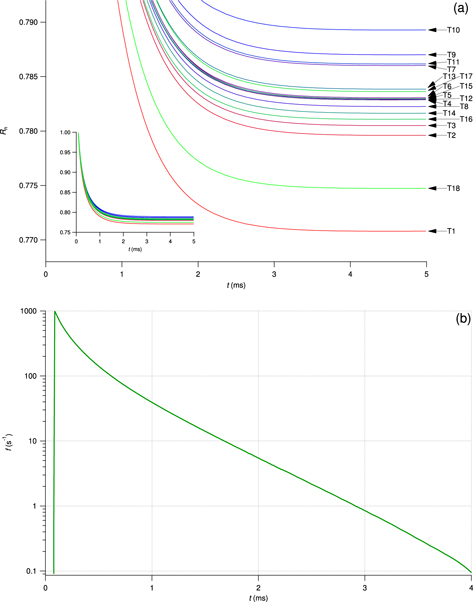
Figure 4. (a) No-follower probability Rn as a function of neutron time delay t, obtained by statistically removing chance coincidences from the time-delay distributions for each of 18 neutron counter tubes in the NM64 at Doi Inthanon, averaging over 2011 January to 2014 February (using 700 electronics). The inset shows Rn over its full range. Note that Rn = 1 at the dead time  and Rn decreases toward a constant value at long t that we call the leader fraction L. Different tubes have different values of L that are due to their location (e.g., L is lower for the edge tubes T1 and T18) and to their different values of td (see text for details). (b) Follower time-delay distribution,
  averaged over eight middle tubes with similar dead times.
Download figure:
Standard image High-resolution imageFor each tube (T1 to T18), Rn = 1 at  and decreases toward an asymptotic value of
  (see inset to Figure 4(a)), providing the second technique for finding L. We found that L can be different for different tubes due to their location and their dead time. Tubes T1 and T18 are at the edges of the row of 18 tubes and have substantially lower values of L. Their count rates are also lower than those of the inner tubes, by about 14%, because they only register counts from nuclear interactions in their surrounding lead rings and rings to one side, lacking a contribution from the other side. Recall that our time-delay histograms are for repeated neutron counts in the same tube, and the leader fraction represents the inverse of multiplicity in the same tube. Counts from nuclear interactions in lead rings to the side produce less multiplicity in the tube of interest, so edge tubes, with fewer counts from lead rings to the side, have a higher average multiplicity and a lower leader fraction L. In fact, the next-to-edge tubes T2 and T17, and to some extent T3 and T16, also have a lower L value than middle tubes with the same dead time td, which is the other factor affecting L. Because of different electronic components, tubes 7, 9–11, 17, and 18 have td = 88 to 91 μs, while the other tubes have td = 80 to 83 μs. Figure 4(a) shows that a longer value of td results in a greater L value. This is because a longer dead time reduces the multiplicity (see also Aiemsa-ad et al. 2015), hence the greater L.
Figure 4(b) shows the follower time-delay histogram  averaged over eight middle tubes with similar (shorter) dead times, namely, tubes 4–6, 8, and 12–15, again using data from 2011 January to 2014 February. This represents the time-delay distribution for neutron counts that follow another neutron count in the same tube from the same atmospheric secondary, removing the effect of chance coincidences. The integral of this function is the follower fraction:
  Monte Carlo simulations of NM64 response to cosmic-ray showers can readily model the distribution
  considering only follower counts, to compare with this measured distribution. The middle portion of this log–linear plot is roughly a straight line, corresponding to a distribution
  for
for  ms, which relates to the absorption timescale for neutrons generated by nuclear interactions inside the monitor. Our results concerning f(t) are similar to those of Hatton (1971).
Note that there were some NM, especially in Russia and the former Soviet Union, that used a long dead time with the aim of eliminating multiplicity (Bieber et al. 2004) so that the interaction of one atmospheric secondary particle in the NM would yield one count. The NM at Apatity, Russia, provides two types of count rates, with a long dead time of 1.2 ms and a short dead time of 10 μs, in order to provide direct information about the role of multiplicity (Balabin et al. 2015). However, based on Figure 4, we see that the dead time of 1.2 ms actually still allows a substantial portion of follower pulses to be counted. A dead time of ∼4 ms would be more effective in eliminating the follower counts and ensuring a multiplicity very close to 1.
Our third technique for estimating L from a time-delay histogram is to divide α, the decay rate of the exponential at long t, which represents the rate of chance coincidences from new leader counts, by the measured count rate from leaders and followers. All three estimates yield similar values of L, which increases our confidence in the analysis techniques. For further analysis we use the first estimate, which is simple and robust.
In greater detail, the first technique for determining L from a given time-delay histogram should also take into account the overflow time to = 142 ms in the electronic recording system. Then the recorded probability density  is given by

For  we use
The long-time histogram is fit to an exponential form  using a maximum likelihood method that accounts for the Poisson distribution in the observed
  for each time bin t. We then determine L from the fit parameters using

3.2. Correction of the Leader Fraction
Before determining the leader fraction for data from the 600 electronics (2007 December to 2011 January), it was necessary to correct for a first-pulse bias. This bias occurred because those electronics record time delays (and pulse heights) for only the first 16 neutron pulses per second from each tube. At Doi Inthanon, the count rate in the 18NM was about 34 Hz per tube, so time delays were not recorded for some of the counts. To understand the first-pulse bias, consider the sequence of neutron pulses from one counter tube. The sequence is random relative to the start of a new second, when time delays will be recorded; conversely, we can view that the new second starts at a random time relative to the sequence of neutron counts. A given pulse will be the first of a new second if the second starts during the time interval between that pulse and the preceding one, the duration of which is simply the time delay t for that pulse. In the sequence of neutron pulses, the probability that the new second starts before the pulse of interest is proportional to t. This is the first-pulse bias: the probability distribution of t for the first pulse in each second is proportional to the average distribution multiplied by t.
If the electronics could record time delays for all neutron pulses, the total time-delay distribution would have no bias. Effectively, the bias toward higher t for the first pulse would be offset by a bias toward lower t for each distribution of kth pulses in the second, with  This bias is negligible when k is much smaller than the average number of pulses per second per tube but becomes more important for higher k. Because the 600 electronics were able to record 16 out of the
  pulses per second per tube, only the first-pulse bias is important. We corrected the histograms for this bias before performing the analysis.
The 700 electronics (used from 2011 January to 2014 February) can record up to 48 pulse heights per second, and therefore most seconds had no bias. The exception was that, as noted earlier, 1 s out of every 30 was devoted to housekeeping, and the pulse heights arriving during that second were stored and transmitted during the following second. Therefore, during the following second, the electronics would record time delays for 48 of the  stored and new pulses, again resulting in a first-pulse bias. Nevertheless, this occurred for only one pulse per tube every 30 s, corresponding to about 0.1% of the pulses. This has a negligible effect on the time-delay analysis, and we do not correct for this in the data from the 700 electronics.
The leader fraction was determined for each time-delay histogram, i.e., for each counter tube and each time interval, as described in the previous section. Then, to discard results from problematic histograms or inappropriate fits, some cleaning was performed on A and α independently before applying Equation (9) by calculating the ratios of the value for each tube to the all-tube average for the same time period and discarding outliers. Daily averages were computed tube by tube before taking the average over the 18 tubes.
The resulting daily "uncorrected" data for L are plotted in Figure 5(b) (gray curve) in comparison with other daily data for Doi Inthanon: the neutron monitor count rate (Figure 5(a)), the "bare/NM" count-rate ratio of three bare counters to the 18NM (Figure 5(c)), atmospheric water vapor partial pressure (Ew; Figure 5(d)), and atmospheric (barometric) pressure (P, Figure 5(e)). Neutron monitor count rates are well known to require correction for the variation of atmospheric depth, which is well represented by the variation of P as measured by a Digiquartz barometer at PSNM. We convert the uncorrected NM count rate (light blue) to the corrected rate (dark blue) by multiplying with ![$\mathrm{exp}[\beta (P-{P}_{0})],$](https://content.cld.iop.org/journals/0004-637X/817/1/38/revision1/apj522064ieqn49.gif) for a pressure coefficient
for a pressure coefficient  mm Hg−1 and standard pressure
  The NM count-rate correction is performed on an hourly basis, and Figure 5(a) shows daily averages of the hourly rates.

Figure 5. Daily data for Doi Inthanon from 2007 December to 2014 February: (a) 18-tube NM count rate, uncorrected (light blue) and corrected (dark blue) for atmospheric pressure. The corrected count rate is a measure of the cosmic-ray flux above the cutoff rigidity, including a long-term variation associated with the solar activity cycle, and strong short-term Forbush decreases due to solar storms. (b) Leader fraction (L) calculated from the 18 tubes, uncorrected (gray) and corrected (black) for atmospheric pressure and water vapor. The corrected L value indicates the spectral index of primary GCRs, with short-term spectral hardening during the stronger Forbush decreases. The shift in the L value during 2011 January is associated with the upgrade from 600 to 700 electronics. (c) Count-rate ratio of three bare counters to the 18-tube NM, which is strongly anticorrelated with atmospheric water vapor. (d) Atmospheric water vapor pressure (Ew) inferred from the GDAS database. (e) Atmospheric pressure (P) measured at the PSNM station.
Download figure:
Standard image High-resolution imageSimilarly, we expect that L should also require correction for atmospheric effects. A clear yearly wave appears in the uncorrected value of L, which is qualitatively similar to that of the uncorrected NM count rate. However, the wave in uncorrected L does not exactly match the yearly pressure variation.
An important clue about how to correct L comes from the bare/NM ratio at Doi Inthanon in comparison with data from the Global Atmospheric Data Assimilation (GDAS) database.10 We used the relative humidity H (in %) and temperature T (in °C) from the GDAS database for a pressure level of 750 hPa at the four surrounding degree-scale spatial grid points and interpolated these to the geographic location of PSNM. We then used the formula
to infer the atmospheric water vapor pressure Ew. The GDAS data are available at 6 hr intervals, so Ew is calculated at 6 hr intervals, and its daily average is shown in Figure 5. This figure indicates a remarkable anticorrelation between bare/NM and Ew. Apparently the yearly wave in the bare/NM data, with a peak-to-peak amplitude of  can be attributed to water in the environment. This makes it difficult to interpret variations in the bare/NM ratio at Doi Inthanon over timescales of days or longer in terms of cosmic-ray spectral variations, and it provides an important clue that L may be sensitive to Ew as well.
We find that the yearly wave in the uncorrected L value is well explained by the effects of both P and Ew. The atmospheric pressure P has a yearly wave and also has characteristic 24 hr and 12 hr oscillations due to atmospheric tides. Therefore we can use these short-term variations, not present in Ew, to characterize and remove the effect of atmospheric depth. We fit  versus
  for each tube j to straight lines of slope bj. Here Δ denotes the residual with respect to a 24 hr moving average, which isolates short-period oscillations in
  and P while averaging out what are typically slower variations in
  due to Ew or the primary cosmic-ray spectrum. The (positive) correlation in these plots is small but significant. We find values for bj to be in the range 0.015%–0.023% mm Hg−1. The values of Lj are then multiplied by
 ![$\mathrm{exp}[-{b}_{j}(P-{P}_{0})]$](https://content.cld.iop.org/journals/0004-637X/817/1/38/revision1/apj522064ieqn57.gif) to eliminate the pressure dependence.
to eliminate the pressure dependence.
Then we also correct for the atmospheric water vapor partial pressure Ew. The correlation between L and Ew is negligible at low Ew but becomes stronger at higher Ew. To model this nonlinear dependence, we fit the pressure-corrected Lj versus Ew to a power law such that

We obtain  0.001–0.002 and
  1.1–3.0. For reference values, we use
  and
and  which correspond to the averages of P and Ew during the month of January at Doi Inthanon and are appropriate for representing dry-season conditions. Each Lj can then be "vapor corrected" by dividing it by the term in square brackets in Equation (11). We perform the pressure and vapor correction to Lj for each tube and for each time-delay histogram interval, i.e., for daily histograms up to 2009 June 29 and for hourly histograms thereafter, in which case values of Ew for 6 hr intervals were interpolated to derive hourly values. The corrected hourly Lj values were then converted to daily averages for further analysis. The average L of the 18 individual Lj values is shown in Figure 5(b), both before (gray trace) and after (black trace) pressure and vapor correction.
In Figure 5(a), the pressure-corrected PSNM count rate still seems to have a very slight yearly wave, possibly due to a small influence of Ew on the count rate. In our preliminary investigation of such an effect, we find that it does not influence the analysis of the count rate regarding short-term GCR variations in the present work. In further work we will investigate whether the count rate can reliably be vapor corrected, which might be important for interpretation of long-term (monthly or longer) variations.
4. SHORT-TERM VARIATIONS IN THE LEADER FRACTION AND COSMIC-RAY SPECTRUM
The average corrected leader fraction L (Figure 5(b), black trace) has no obvious yearly wave or correlation with environmental factors and is believed to relate to the cosmic-ray spectrum. There was a drop in 2011 January, corresponding to the change from 600 to 700 electronics. Aside from that, and a few remaining glitches, the leader fraction is seen to vary in association with changes in the cosmic-ray flux, and indeed it is expected that changes in the cosmic-ray spectrum occur because of events or processes that also change the flux.
To be more precise, a harder spectrum of primary cosmic rays should produce a harder spectrum of atmospheric secondaries. When the secondaries interact in the NM producer (mostly in the lead), a harder spectrum should lead to a greater average multiplicity and a lower leader fraction. Therefore, a lower leader fraction is associated with a harder cosmic-ray spectrum. Thus, a lower leader fraction indicates a lower spectral index of cosmic rays such as  where j is the cosmic-ray flux as a function of rigidity P.
The GCR flux varies due to solar effects on various timescales. The longest are the 11-year variation in association with the sunspot cycle and the 22-year variation with the solar magnetic cycle (Forbush 1954; Jokipii & Thomas 1981; Nuntiyakul et al. 2014; Abe et al. 2015), which are collectively known as solar modulation. Near sunspot maximum, the solar wind and interplanetary magnetic field are stronger, the tilt angle of the heliospheric current sheet increases, and there are frequent coronal mass ejections that can have even stronger magnetic fields and can drive solar wind turbulence, all of which lead to less diffusion of GCRs into the inner heliosphere. Solar modulation accounts for the long-term trends in Figure 5(a), in which the corrected PSNM count rate reached a maximum in late 2009 and has mostly declined thereafter.
The GCR spectrum also changes with the sunspot cycle and solar activity cycle because solar modulation is stronger at lower energy (Nuntiyakul et al. 2014; Abe et al. 2015). In other words, the GCR spectrum inside the heliosphere is lower than that in interstellar space (Burlaga & Ness 2014), and the reduction is greater at lower energy and at times of solar maximum. Therefore, the GCR spectrum becomes harder during times of lower flux. This is a general property of any GCR decrease in association with solar activity or an enhanced solar wind speed: the decrease is stronger for GCRs of lower energy, so the spectrum is harder at times of GCR flux decrease.
The variations in the corrected leader fraction from the PSNM data match this expectation. In Figure 5(b), the long-term trend (not including the drop in 2011 January, due to the change in electronics) is that L is lower during times of lower GCR flux, indicating a lower spectral index and harder spectrum.
Over shorter timescales, less than one year, we again see that temporary GCR flux decreases are often accompanied by substantial decreases in L, indicating spectral hardening. Interestingly, there are some short-term GCR flux decreases for which there is little or no change in the corrected L value. Examples include the flux decreases of 2011 June 17 and 24 and 2013 June 25. Thus the PSNM leader fraction is not merely parroting the count rate, but rather provides additional information about which flux decreases involved stronger spectral changes at a (vertical) cutoff rigidity of 16.8 GV.
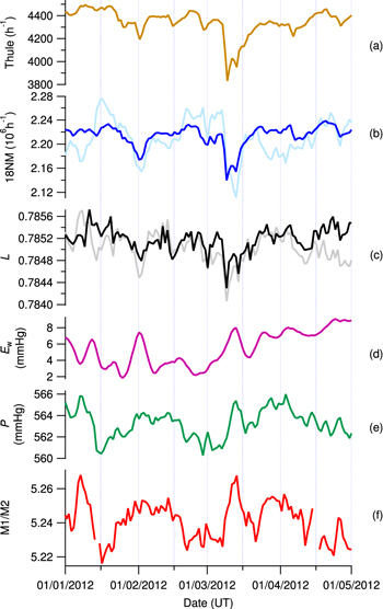
As an example showing different spectral features, Figure 6 presents daily data from 2012 January to April. Figure 6(a) shows the corrected count rate at Thule, Greenland, and the other traces are data for Doi Inthanon, Thailand. Note the compressed vertical scale for Thule; actually, the percentage decreases in the GCR flux at Thule are much greater than at Doi Inthanon. This is because Thule has a much lower cutoff rigidity. In fact, the geomagnetic cutoff is so low that the response to primary cosmic rays is instead limited by an atmospheric cutoff at ∼1 GV.
Figure 6. Daily data from 2012 January to April: (a) 18-tube NM count rate (normalized) at Thule, Greenland, corrected for atmospheric pressure. Daily data from Doi Inthanon: (b) 18-tube NM count rate, uncorrected (light blue) and corrected (dark blue) for atmospheric pressure. (c) Leader fraction (L) calculated from the 18 tubes, uncorrected (gray) and corrected (black) for atmospheric pressure and water vapor. (d) Atmospheric water vapor pressure (Ew) inferred from the GDAS database. (e) Atmospheric pressure (P) measured at the PSNM station. (f) Ratio of rates at multiplicity 1 (M1) to multiplicity 2 (M2). For two Forbush decreases (minimum count rates on 2012 February 1 and 2012 March 8), L also decreases, indicating spectral hardening as expected. The decrease in L is much stronger on March 8, which is consistent with the much stronger decrease at Thule compared with the decrease at Doi Inthanon. Thus the change in L indicates the degree of spectral hardening in a matter consistent with the ratio between Thule and Doi Inthanon count rates. In contrast, the multiplicity ratio M1/M2 is dominated by chance coincidences and does not correctly indicate spectral hardening during these Forbush decreases.
Download figure:
Standard image High-resolution image
Figure 6 shows a sequence of several GCR decreases, and each clear decrease in the Doi Inthanon corrected NM count rate was associated with a decrease in the corrected leader fraction L. The most notable features are two Forbush decreases due to solar storms, with minimum GCR flux on 2012 February 1 and 2012 March 8. The latter decrease, which includes the lowest NM count rate and the lowest L in these six years of data (see Figure 5), had a complex time profile with a second minimum on 2012 March 12.
The leader fraction decrease indicates much stronger spectral hardening on 2012 March 8 than during the 2012 February 1 event. To verify this conclusion, we also compare the NM count rate at Doi Inthanon with that from Thule (atmospheric cutoff 1 GV). Indeed, the Thule decrease on 2012 March 8 was much stronger than all the other decreases, while at Doi Inthanon the decrease on 2012 March 8 was only moderately stronger than that on 2012 February 1. The stronger decrease in GCR at lower rigidity on 2012 March 8 indicates stronger spectral hardening, which verifies the information provided by L. Note also that at Thule there was a sharp increase after 2012 March 8 followed by the second decrease, while at Doi Inthanon these features were relatively weaker, so these features should correspond to spectral changes. Indeed, L did sharply recover after 2012 March 8 and decreased again after the second flux decrease. These observations provide useful confirmation based on independent data that the degree of change in the leader fraction does indicate the degree of change in the primary cosmic-ray spectrum.
Finally, Figure 6(f) shows the ratio of count sequences with multiplicity 1 divided by those with multiplicity 2, i.e., M1/M2. In our electronics, the multiplicity is measured as the total number of neutron counts in the same tube during a time window of  ms after a given count, and after that time window a new time window begins with the first new count. In principle, a higher multiplicity should indicate more energetic primary cosmic rays, so the M1/M2 ratio would seem to be a possible indicator of spectral changes in the same sense as L (i.e., a decrease could indicate spectral hardening). However, in practice we find that M1 and M2 at Doi Inthanon as defined in terms of this time window are dominated by chance coincidences. For a given uncorrected count rate N, for chance coincidences alone M1/M2 is roughly proportional to
  Since the uncorrected count rate is strongly inversely correlated with atmospheric pressure P, we see in Figure 6 that M1/M2 varies very much like P. This variation in M1/M2 does not reflect the variation of the cosmic-ray spectrum, and after 2012 March 8, M1/M2 happens to vary in the opposite sense from that expected for spectral hardening. We have also tried to develop a pressure correction for M1/M2 but have not obtained a useful indicator of cosmic-ray spectral variations. This stresses the importance of techniques to remove the effects of chance coincidences when determining quantities related to multiplicity, such as the leader fraction.
5. SUMMARY AND DISCUSSION
Here we have presented the first use of NM time-delay histograms to track cosmic-ray spectral variations as a function of time. We have developed analysis techniques to statistically remove the effect of chance coincidences and extract the leader fraction L, which indicates the cosmic-ray spectral index. We have been able to correct L for environmental variables, and independent data confirm that it can indicate the degree of GCR spectral changes during Forbush decreases. This represents a new capability for a single NM station to track GCR spectral variations, avoiding the systematic uncertainties associated with comparing data from different locations. We implemented this capability in the PSNM at Doi Inthanon, Thailand, which has the world's highest cutoff rigidity for a fixed NM station. Therefore, estimation of the cosmic-ray spectral index above this cutoff provides unique information that is not accessible when comparing data from different NM stations.
The leader fraction is a measure of the inverse multiplicity, after removing the effect of chance coincidences. We have shown that this can provide a much more accurate indication of cosmic-ray spectral variations when compared with the multiplicity as defined in terms of the number of counts arriving within a specific time window, which in some cases (such as for PSNM) is dominated by chance coincidences. The determination of L also avoids an arbitrary specification of the time window. Nevertheless, the extraction of L from time-delay histograms is still affected by the capabilities of the hardware and electronics, such as the dead time. Further work is needed to calibrate changes in L in terms of changes in the GCR spectral index.
The neutron time-delay histograms represent a combination of effects of chance coincidences (at long time delays; see Figure 3(b)) and the multiplicity effect, in which there are "follower" neutron counts after an initial count in the same counter tube from the same atmospheric secondary particle (Bieber et al. 2004). We have developed three techniques to determine the leader fraction of counts that are not followers. The simplest measure of L is directly proportional to the amplitude of the exponential tail from chance coincidences. In addition, we also measured  the follower time-delay distribution with chance coincidences statistically removed (Figure 4(b)), which could conveniently be compared with Monte Carlo simulations for independent atmospheric secondary particles.
We have also examined the count-rate ratio of bare neutron counters to the 18NM64 at Doi Inthanon, i.e., the bare/NM ratio. In principle, this ratio can also indicate cosmic-ray spectral variations. For example, the South Pole bare/NM ratio over timescales of hours has been used to indicate the spectral index of relativistic solar particles from several solar storms (e.g., Bieber & Evenson 1991; Bieber et al. 2002, 2013). Ruffolo et al. (2006) compared the spectral index as a function of time during the event of 1989 October 22 as inferred from the South Pole bare/NM ratio with that inferred by Cramp et al. (1997) using data from the worldwide NM network, including stations at different cutoff rigidities, and the results were in very good agreement.
At Doi Inthanon, we have found variations in bare/NM over timescales longer than a few days to be strongly anticorrelated with the atmospheric water vapor pressure, resulting in a seasonal variation in bare/NM of amplitude  Furthermore, Figure 5 indicates a memory effect, in which the seasonal variation in bare/NM can take ∼1 to 2 months to respond to some changes in Ew, such as during 2009 April to June. This could be due to the effect of water accumulation in the concrete, rocks, and ground surrounding the PSNM building. Over timescales of weeks to months, Ew can serve as a proxy for rainfall, and the observed memory effect could be due to subsurface water that accumulates with time when Ew initially rises at the start of the rainy season (which lasts roughly from May through October). The same property that makes bare counters useful for spectral determination, their sensitivity to low-energy secondary neutrons, also makes them sensitive to water in the environment, which can moderate and absorb such neutrons. In fact, unshielded neutron counters are widely used to measure soil moisture (Zreda et al. 2008) and can be sensitive to soil moisture over ∼100 m (Köhli et al. 2015). Because of this environmental sensitivity, it is difficult to use bare/NM at Doi Inthanon to measure spectral variations over timescales longer than a few days. It could be useful to indicate spectral variations over shorter timescales or in locations with a more constant environment.
These considerations imply that, in principle, Ew could have either a direct effect on L or bare/NM, due to water in the atmosphere, or an indirect effect, such as a proxy for accumulation of rain at or below the surface. As noted above, we suspect that bare/NM mainly has an indirect effect from Ew. Further confirmation comes from an analysis of data from a bare counter at Mahidol University in Bangkok, Thailand, which was mainly used for teaching and for testing electronics. That bare counter is on the fifth floor of a six-story building, and we consider that rain accumulation on the roof should have little effect on the secondary population compared with propagation through the building, so direct effects should persist while indirect effects should mostly be absent. Indeed, there is no apparent yearly wave or association with Ew in those data, supporting the idea that the association of bare/NM at Doi Inthanon with Ew is an indirect effect. In contrast, Ew may have a direct effect on L, which measures the inverse multiplicity of the interactions of energetic secondary particles in the 18NM (mainly secondary neutrons of 10 MeV to 10 GeV in energy) and is rather insensitive to neutrons from the local environment.
Interestingly, L and bare/NM are found to have a nonlinear relationship with Ew, that is, a very weak dependence for low Ew and a much stronger dependence at high Ew. We tentatively attribute this to condensation, which depends nonlinearly on Ew. Condensed water in the atmosphere could have a direct effect on L, such as by moderating a fraction of secondary neutrons more strongly than accounted for by their contribution to atmospheric pressure (which is corrected for). Similarly, rainfall also varies nonlinearly with Ew, and Ew could have an indirect effect on bare/NM associated with rain accumulation.
While several types of data can provide long-term spectral information about GCRs from year to year, it is more challenging to monitor short-term variations. Long-term spectral variations can already be studied by the worldwide NM network, spanning a range of cutoff rigidity from the atmospheric cutoff at ∼1 GV to the maximum vertical geomagnetic cutoff of 16.8 GV, and could be assisted by an extensive intercalibration program (Moraal et al. 2000; Krüger et al. 2008; Aiemsa-ad et al. 2015). Year-to-year spectral variations have been studied by occasional "latitude surveys" of mobile NMs on aircraft or ships traversing a wide range of cutoff rigidity (Moraal et al. 1989; Nuntiyakul et al. 2014). Repeated balloon-borne measurements (e.g., Abe et al. 2015) and long-term space missions provide direct measurements of individual GCR species over different time intervals. These techniques have limited applicability for variations over monthly or daily timescales, such as for the study of Forbush decreases. In the Introduction, we discussed the difficulties in comparing neutron monitor data from different stations over subannual timescales (see Figure 2). By their nature, latitude surveys and balloon-borne experiments are not continuous and require some time to accumulate precise spectra. Similarly, space missions such as PAMELA and AMS-02 require some time to accumulate spectra, especially for energies above 10 GeV, as considered in the present work. So far, their spectra at ∼10 GeV have been presented for one-month intervals (Adriani et al. 2013; Consolandi 2015). Thus, time-delay spectra from NMs provide an attractive means of studying shorter-term spectral variations.
In Figure 6, we used a comparison between Thule and Doi Inthanon data to confirm the relative degree of spectral hardening indicated by decreases in L. While the comparison between monitors can qualitatively confirm the degree of spectral hardening, it remains difficult to quantify the spectral hardening because of the issues illustrated in Figure 2 and also because of a possible anisotropy effect. Note also that the comparison may span a substantial range in cutoff rigidity. The measurement of L has the potential to quantitatively determine the spectral index for a specific cutoff rigidity and "look" direction in space.
Thus the techniques presented here for monitoring GCR spectral variations at a single station can play a useful role in clarifying short-term cosmic-ray variations at a specific cutoff rigidity. Their implementation at the PSNM in Doi Inthanon, Thailand, the NM station with the world's highest geomagnetic cutoff rigidity, provides information about particle energies beyond the cutoff and extends the "reach" of the neutron monitor network to higher rigidity, helping to bridge the gap between the NM network and the muon detector network with median rigidities starting at ∼60 GV.
Construction of the PSNM was made possible by the donation of equipment from Shinshu University, which was facilitated by T. Chiba, N. Yahagi, and H. Takahashi of Iwate University; donation of equipment from the University of Delaware; and support from the Royal Thai Air Force, Mahidol University, Ubol Ratchathani University, Chulalongkorn University, the Thailand Research Fund, and Thai Unique Co., Ltd. We thank TOT Public Co., Ltd. and Chatchai Injai for their kind assistance with the observations. This work was also supported by the Thailand Research Fund and Mahidol University (Grant BRG5880009), a Postdoctoral Fellowship from Mahidol University, and the United States National Science Foundation via awards PLR-1341562, PLR-1245939, and their predecessors. We thank the Yangbajing Neutron Monitor Collaboration for use of their daily count-rate data. We acknowledge Supawit Kittipadakul, Kritpong Kulthamrongsri, Wattanapol Sangpho, and Thawatchai Sudjai of Mahidol Wittayanusorn School for their analysis of bare counter data at Mahidol University and also numerous useful discussions with Roger Pyle and Takao Kuwabara.
Footnotes
- 9
During the course of a Forbush decrease, spectral hardening (a stronger decrease at lower cutoff rigidity) can easily be seen in real-time plots, e.g., at http://neutronm.bartol.udel.edu/~pyle/SpectralPlot.png and http://www.nmdb.eu/?q=node/335
- 10