


ABSTRACT
We present new optical colors for 28 Kuiper Belt objects (KBOs) and 35 Centaur objects measured with the 1.8 m Vatican Advanced Technology Telescope and the 4.3 m Discovery Channel Telescope. By combining these new colors with our previously published colors, we increase the sample size of our survey to 154 objects. Our survey is unique in that the uncertainties in our color measurements are less than half the uncertainties in the color measurements reported by other researchers in the literature. Small uncertainties are essential for discerning between a unimodal and a bimodal distribution of colors for these objects as well as detecting correlations between colors and orbital elements. From our survey, it appears red Centaurs have a broader color distribution than gray Centaurs. We find red Centaurs have a smaller orbital inclination angle distribution than gray Centaurs at the 99.3% confidence level. Furthermore, we find that our entire sample of KBOs and Centaurs exhibits bimodal colors at the  confidence level. KBOs and Centaurs with HV > 7.0 have bimodal colors at the 99.96% confidence level and KBOs with HV < 6.0 have bimodal colors at the 96% confidence level.
Export citation and abstract BibTeX RIS
1. INTRODUCTION
We first reported that Kuiper Belt objects (KBOs) and Centaur objects exhibit two distinct colors—gray and red (Tegler & Romanishin 1998, 2000, 2003; Tegler et al. 2003). Presumably, the two colors indicate two types of surface material—one material that nearly equally absorbs wavelengths of optical light and another material that is more prone to absorbing shorter rather than longer wavelengths of optical light. Complex organic molecules are known to efficiently absorb shorter wavelengths of optical light. So, it is possible optical colors are a proxy for the amount of complex organic molecules on the surfaces of KBOs and Centaurs.
Our two color populations were called into question by other researchers in that they found KBOs and Centaurs exhibit a continuum of colors from gray through red (Barucci et al. 1999; Jewitt & Luu 2001; Hainaut & Delsanti 2002). The ensuing controversy made it difficult to use colors to constrain the relative importance of primordial processes (e.g., a thermal gradient and astrochemistry in the primordial planetary disk) versus evolutionary processes (e.g., collisions and cryovulcanism) on these bodies.
As sample sizes grew, it became possible to examine the color distributions of different dynamical classes. We found cold, classical KBOs are red (Tegler & Romanishin 2000), a result confirmed by other researchers (Jewitt & Luu 2001; Trujillo & Brown 2002; Peixinho et al. 2004). In addition, we found Centaurs divide into gray and red populations (Tegler et al. 2003, 2008). Peixinho et al. (2003) reanalyzed their data and found Centaurs divide into two color populations, but they found no evidence that KBOs divide into two color populations.
More recently, Peixinho et al. (2012) and Peixinho et al. (2015) found support for two color populations of KBOs by compiling and analyzing the B – R colors and HR magnitudes of 253 objects and 354 objects in the literature, respectively, where they used HR as a proxy for object size. They found small and large objects exhibit two color populations at a statistically significant level whereas intermediate sized objects exhibit a continuum of colors. In addition, Fraser & Brown (2012) found small KBOs with perihelia q < 35 au exhibit two optical color populations.
Here we present new optical colors for 28 KBOs and 35 Centaurs taken with the 1.8 m Vatican Advanced Technology Telescope (VATT) and the 4.3 m Discovery Channel Telescope (DCT). We combined these new measurements with our previously published measurements to increase our sample size to 154 KBOs and Centaurs. Our survey is unique in that the uncertainties in our measurements are about half the uncertainties in measurements reported by other groups in the literature. Small uncertainties are essential for discerning between a unimodal and a bimodal distribution of colors as well as detecting correlations between colors and orbital parameters of these objects. We report two interesting results—(1) using a sample size almost twice as large as available in the literature, we find red Centaurs have a smaller orbital inclination angle distribution than gray Centaurs at the 99.3% confidence level, and (2) we find that our entire sample of KBOs and Centaurs exhibits bimodal colors at the  confidence level. KBOs and Centaurs with HV > 7.0 have bimodal colors at the 99.96% confidence level and KBOs with HV < 6.0 have bimodal colors at the 96% confidence level.
The controversy concerning KBO and Centaur colors may be near an end. If so, the colors and magnitudes of these objects may provide important observational constraints on the relative importance of primordial versus evolutionary processes affecting these objects.
2. OBSERVATIONS
2.1. Vatican Advanced Technology Telescope
We obtained observations with the 1.8 m VATT (the Alice P Lennon telescope and Thomas J. Bannan facility) and a CCD camera at the f/9 aplanatic Gregorian focus. For six observing runs between 2003 November and 2006 April, we made use of a 2048 × 2048 pixel CCD with 15 μm pixels. We binned the 15 μm pixels 2 × 2, yielding 1024 × 1024 pixels and covering 6 4 × 64 on the sky at 0
 375 pixel−1. For two observing runs between 2009 November and 2011 November, we made use of a 4064 × 4064 pixel CCD. We binned the 15 μm pixels 2 × 2, yielding 2032 × 2032 pixels and covering 127 × 127 on the sky at 0375 pixel−1. For all runs, we used Harris B (450 nm), V (550 nm), and R (650 nm) glass filters.
2.2. Discovery Channel Telescope
We obtained observations with the 4.3 m DCT and the Large Monolithic Imager (LMI) at the Ritchey–Chretien f/6.1 focus. LMI is a 6144 × 6160 pixel CCD with 15 μm pixels. We binned the 15 μm pixels 2 × 2, yielding 3072 × 3080 pixels and covering 123 × 123 on the sky at 0240 pixel−1. We used Harris B (450 nm), V (550 nm), and R (650 nm) glass filters.
2.3. Observation and Reduction Processes
The VATT and DCT were tracked at the sidereal rate. Individual exposure times were usually 300 s, although for some of the faster moving objects, particularly Centaurs, we observed with 90, 120, or 180 s exposure times to keep object motion over an individual exposure smaller than 05. To minimize lightcurve effects, we obtained images with a filter sequence of RRVVBBBBVVRR. The sequence was repeated up to four times for some of the fainter objects. For each object, we used the same exposure time in each filter. We observed standard stars (Landolt 2009; Clem & Landolt 2013) each night and derived atmospheric extinction coefficients and transformation equations for each run. All observations were made under photometric conditions. Further details concerning our observing and reduction procedures are described in Tegler & Romanishin (1997, 1998, 2000, 2003).
We present findings from our observations in Table 1. The first column gives the number of the object, if one was assigned to it. The second column gives the provisional designation of the object, or its name if one was assigned to it. In column 3, we give the UT dates at the midpoint times of the observations. In column 4, we give the time intervals of the observations in hours. In columns 5–7, we give the heliocentric distances in AU (r), geocentric distances in AU (Δ), and solar phase angles in degrees (α) at the midpoint observation times. The objects are ordered by UT date. The last 12 objects were observed with the DCT. Most objects were observed on a single night during a single run, but five were observed on two nights during the same run, and one object (60558) was observed during two separate runs.
Table 1. Journal of Observations
| Number | Designation/Name | UT Date | Span | r | Δ | α |
|---|---|---|---|---|---|---|
| (hr) | (au) | (au) | (deg) | |||
| 469372 | 2001 QF298 | 2003 Nov 22.18 | 1.4 | 42.704 | 42.373 | 1.25 |
| ⋯ | ⋯ | 2003 Nov 24.13 | 2.5 | 42.705 | 42.406 | 1.26 |
| 55637 | 2002 UX25 | 2003 Nov 24.22 | 1.6 | 42.530 | 41.738 | 0.80 |
| 55638 | 2002 VE95 | 2003 Nov 24.31 | 1.2 | 28.010 | 27.050 | 0.47 |
| 84922 | 2003 VS2 | 2003 Nov 24.37 | 1.2 | 36.432 | 35.479 | 0.41 |
| 55565 | 2002 AW197 | 2003 Nov 24.45 | 1.8 | 47.176 | 46.899 | 1.16 |
| 90482 | Orcus | 2004 Apr 20.17 | 1.8 | 47.619 | 47.227 | 1.12 |
| 47932 | 2000 GN171 | 2004 Apr 20.31 | 1.8 | 28.516 | 27.515 | 0.17 |
| 26181 | 1996 GQ21 | 2004 Apr 22.34 | 2.9 | 39.873 | 38.876 | 0.19 |
| 60558 | Echeclus | 2004 Apr 23.21 | 2.0 | 14.023 | 13.135 | 1.98 |
| 55576 | Amycus | 2004 Apr 23.32 | 1.2 | 15.241 | 14.278 | 1.12 |
| 469362 | 2001 KB77 | 2004 Apr 24.35 | 2.7 | 30.955 | 29.964 | 0.34 |
| 120181 | 2003 UR292 | 2004 Dec 11.16 | 2.6 | 27.029 | 26.641 | 1.93 |
| ⋯ | ⋯ | 2004 Dec 12.10 | 1.5 | 27.029 | 26.656 | 1.94 |
| 90377 | Sedna | 2004 Dec 11.29 | 2.5 | 89.236 | 88.411 | 0.34 |
| 208996 | 2003 AZ84 | 2004 Dec 11.40 | 1.2 | 45.766 | 44.921 | 0.64 |
| 416400 | 2003 UZ117 | 2004 Dec 12.19 | 2.0 | 39.701 | 38.923 | 0.88 |
| 2002 XV93 | 2004 Dec 12.42 | 1.6 | 40.359 | 39.400 | 0.32 | |
| 136204 | 2003 WL7 | 2004 Dec 13.11 | 1.9 | 15.806 | 15.183 | 2.82 |
| 84522 | 2002 TC302 | 2004 Dec 13.20 | 1.8 | 47.769 | 47.156 | 0.93 |
| 33340 | 1998 VG44 | 2004 Dec 13.30 | 1.9 | 29.820 | 28.858 | 0.40 |
| 84719 | 2002 VR128 | 2004 Dec 14.19 | 1.8 | 36.035 | 35.351 | 1.13 |
| 120216 | 2004 EW95 | 2005 Jun 06.20 | 1.3 | 28.309 | 27.822 | 1.81 |
| ⋯ | ⋯ | 2005 Jun 07.19 | 1.4 | 28.309 | 27.837 | 1.83 |
| 307261 | 2002 MS4 | 2005 Jun 06.36 | 2.2 | 47.426 | 46.460 | 0.39 |
| 119951 | 2002 KX14 | 2005 Jun 07.28 | 1.9 | 39.615 | 38.645 | 0.43 |
| ⋯ | ⋯ | 2005 Jun 08.25 | 1.5 | 39.615 | 38.650 | 0.45 |
| 167P | CINEOS | 2005 Jun 07.41 | 1.8 | 12.410 | 11.970 | 4.31 |
| ⋯ | ⋯ | 2005 Jun 08.44 | 0.8 | 12.410 | 11.955 | 4.27 |
| 90568 | 2004 GV9 | 2005 Jun 08.19 | 1.2 | 39.003 | 38.342 | 1.14 |
| 136199 | Eris | 2005 Oct 31.33 | 1.8 | 96.896 | 95.980 | 0.22 |
| 119979 | 2002 WC19 | 2005 Nov 01.40 | 2.0 | 43.468 | 42.627 | 0.71 |
| 136472 | Makemake | 2006 Apr 02.16 | 0.9 | 51.932 | 51.116 | 0.64 |
| 120132 | 2003 FY128 | 2006 Apr 02.25 | 1.7 | 38.120 | 37.204 | 0.18 |
| 60558 | Echeclus | 2006 Apr 02.36 | 1.0 | 12.904 | 11.910 | 0.47 |
| 174567 | Varda | 2006 Apr 02.45 | 1.2 | 48.207 | 47.654 | 1.00 |
| 250112 | 2002 KY14 | 2009 Nov 17.16 | 1.5 | 8.640 | 8.228 | 6.11 |
| 2007 VH305 | 2009 Nov 17.27 | 2.7 | 8.249 | 7.288 | 1.71 | |
| 309741 | 2008 UZ6 | 2009 Nov 17.40 | 3.0 | 10.814 | 9.830 | 0.55 |
| 2002 QX47 | 2009 Nov 18.16 | 3.5 | 20.386 | 19.876 | 2.41 | |
| 309737 | 2008 SJ236 | 2009 Nov 18.30 | 2.2 | 6.158 | 5.170 | 0.44 |
| 145486 | 2005 UJ438 | 2009 Nov 18.42 | 3.1 | 8.315 | 7.629 | 5.13 |
| 315898 | 2008 QD4 | 2009 Nov 20.14 | 1.5 | 5.574 | 4.930 | 8.19 |
| 346889 | Rhiphonos | 2009 Nov 20.22 | 1.9 | 6.025 | 5.328 | 7.08 |
| 309139 | 2006 XQ51 | 2009 Nov 20.32 | 2.2 | 12.661 | 11.813 | 2.38 |
| 2007 UM126 | 2009 Nov 21.15 | 1.7 | 11.900 | 11.160 | 3.25 | |
| 2007 RH283 | 2009 Nov 21.27 | 1.4 | 18.444 | 17.638 | 1.81 | |
| 248835 | 2006 SX368 | 2011 Oct 28.19 | 2.3 | 12.089 | 11.413 | 3.55 |
| 445473 | 2010 VZ98 | 2011 Oct 28.32 | 3.0 | 37.484 | 36.493 | 0.12 |
| 342842 | 2008 YB3 | 2011 Oct 28.45 | 0.7 | 6.576 | 6.502 | 8.69 |
| 2009 YG19 | 2011 Oct 30.40 | 2.4 | 33.803 | 32.933 | 0.83 | |
| 336756 | 2010 NV1 | 2011 Oct 31.13 | 1.6 | 9.583 | 9.088 | 5.29 |
| 2010 BK118 | 2011 Oct 31.19 | 0.7 | 6.234 | 5.384 | 5.08 | |
| 143707 | 2003 UY117 | 2011 Oct 31.26 | 2.3 | 32.861 | 31.875 | 0.20 |
| 447178 | 2005 RO43 | 2011 Oct 31.36 | 2.3 | 24.822 | 23.935 | 1.05 |
| 341275 | 2007 RG283 | 2011 Nov 01.15 | 2.3 | 17.346 | 16.485 | 1.67 |
| 382004 | 2010 RM64 | 2011 Nov 01.23 | 0.8 | 6.475 | 5.684 | 5.65 |
| 2002 PQ152 | 2014 Oct 26.32 | 2.8 | 22.921 | 21.950 | 0.54 | |
| 463368 | 2012 VU85 | 2014 Oct 26.43 | 1.8 | 25.690 | 24.938 | 1.48 |
| 471339 | 2011 ON45 | 2014 Oct 28.18 | 1.2 | 10.395 | 9.671 | 3.89 |
| ⋯ | ⋯ | 2014 Oct 29.20 | 1.7 | 10.394 | 9.683 | 3.96 |
| 2007 TK422 | 2014 Oct 28.29 | 1.8 | 22.790 | 21.801 | 0.23 | |
| 449097 | 2012 UT68 | 2014 Oct 28.36 | 0.8 | 12.668 | 11.772 | 2.03 |
| 2010 TH | 2014 Oct 28.39 | 0.8 | 15.943 | 15.128 | 2.10 | |
| 2013 UL10 | 2014 Oct 28.42 | 0.7 | 6.230 | 5.462 | 6.20 | |
| 349933 | 2009 YF7 | 2014 Oct 28.47 | 1.1 | 8.839 | 8.558 | 6.29 |
| 459971 | 2014 ON6 | 2014 Oct 29.10 | 0.7 | 6.186 | 5.937 | 9.10 |
| 2007 TJ422 | 2014 Oct 29.33 | 3.1 | 18.905 | 17.914 | 0.17 | |
| 281371 | 2008 FC76 | 2014 Oct 29.41 | 0.5 | 10.197 | 9.234 | 1.44 |
| 459865 | 2013 XZ8 | 2014 Oct 29.46 | 1.1 | 11.508 | 11.189 | 4.75 |
Object 60558, also known by its cometary designation 174P/Echeclus, was observed on two nights separated by about two years. The first observation in 2004 April was before the cometary outburst of the object discovered by Choi & Weismann (2006) in 2006 January. Our 2006 April observation was taken when the object showed a complex coma (Tegler et al. 2006). However, the nucleus appeared stellar in our images, and measurements of the nucleus with various sized apertures indicate no significant contamination due to the coma. This object had another outburst in 2011 May (Jaeger 2011).
167P/CINEOS has a cometary designation, but unlike 174P/Echeclus, it has no minor planet number. This object was first reported as an asteroidal object, designated 2004 PY42, but was found to have a very faint coma (Romanishin & Tegler 2005). Green (2005) discusses the designation of this object. This object has orbital parameters broadly similar to those of (2060) 95P/Chiron, which is accepted as a Centaur and so we see no reason not to include 167P/CINEOS among the Centaurs.
Although most of the calibration and derivation of transformation equations between instrumental and standard magnitudes followed the techniques presented in Tegler & Romanishin (1997, 1998, 2000, 2003), we did use a somewhat different technique to derive the average instrumental magnitudes of the objects. The instrumental magnitude of each exposure at midpoint time t, corrected to "total" magnitude using the aperture correction technique and corrected for atmospheric extinction, (mI(t)), was plotted versus the observed UT midpoint time. For the filter with the longest time span, almost always the R filter, we fit a curve by least squares to the mI(t) points. Depending on the apparent variation of magnitude with time, we used one of three fits: (1) a constant mI(t), (2) a simple linear fit

or, (3) a linear plus parabolic curve

where a and b are constants.
This curve, without change of shape, was then fit by least squares to the mI(t) in the other filters by shifting the magnitude to determine the magnitude offsets from the first filter and from these offsets instrumental colors were found. Of course, this procedure assumes that the color is constant over the time period of observation. An example is shown Figure 1 for 309139, where the linear plus parabolic curve was needed to fit the obvious curvature in the magnitude versus time points.

Figure 1. Instrumental magnitudes in R, V, and B, corrected to zero airmass, vs. time.
Download figure:
Standard image High-resolution imageAn estimate of the uncertainty in the overall magnitude fit in each filter was derived from the scatter (σ) of the mI(t) around the fit line, the number of points, and the number of degrees of freedom of the fit. The uncertainty in each color was estimated as the square root of the sum of 0.012 and the squares of the uncertainties in the two filters. The 0.01 mag is included as an estimate of the uncertainty introduced by the fit to the color equations.
Measurements for the individual nights for objects observed on more than one night are given in Table 2. Comparison of the differences between the colors on different nights and our estimated uncertainties allows a check on our internal uncertainty estimates. The absolute value of the differences between pairs of randomly chosen normally distributed numbers should be ∼1.4σ. For the 21 color difference pairs in Table 2, the absolute difference divided by the average uncertainty of the pair is 1.3, showing that our uncertainty estimates are reasonable.
Table 2. Objects Observed on Two Nights
| Number | Designation/Name | Date | H
|
Vobs |

|

|

|
|---|---|---|---|---|---|---|---|
| 469372 | 2001 QF298 | 2003 Nov 22 | 5.27 | 21.74 | 0.79 ± 0.07 | 0.32 ± 0.06 | 1.10 ± 0.07 |
| ⋯ | ⋯ | 2003 Nov 24 | 5.37 | 21.84 | 0.71 ± 0.06 | 0.47 ± 0.06 | 1.18 ± 0.06 |
| 60558 | Echeclus | 2004 Apr 23 | 9.72 | 21.29 | 0.86 ± 0.04 | 0.56 ± 0.03 | 1.41 ± 0.04 |
| ⋯ | ⋯ | 2006 Apr 02 | 9.60 | 20.63 | 0.78 ± 0.10 | 0.51 ± 0.06 | 1.29 ± 0.09 |
| 120181 | 2003 UR292 | 2004 Dec 11 | 7.56 | 22.08 | 1.01 ± 0.09 | 0.74 ± 0.07 | 1.75 ± 0.08 |
| ⋯ | ⋯ | 2004 Dec 12 | 7.46 | 21.98 | 1.04 ± 0.09 | 0.53 ± 0.07 | 1.58 ± 0.09 |
| 120216 | 2004 EW95 | 2005 Jun 06 | 6.42 | 21.12 | 0.70 ± 0.03 | 0.35 ± 0.02 | 1.06 ± 0.03 |
| ⋯ | ⋯ | 2005 Jun 07 | 6.50 | 21.21 | 0.69 ± 0.03 | 0.40 ± 0.03 | 1.09 ± 0.03 |
| 119951 | 2002 KX14 | 2005 Jun 07 | 4.84 | 20.85 | 1.08 ± 0.03 | 0.60 ± 0.02 | 1.68 ± 0.03 |
| ⋯ | ⋯ | 2005 Jun 08 | 4.89 | 20.91 | 1.01 ± 0.04 | 0.61 ± 0.02 | 1.62 ± 0.04 |
| 167P | CINEOS | 2005 Jun 07 | 9.83 | 21.08 | 0.78 ± 0.05 | 0.52 ± 0.03 | 1.30 ± 0.04 |
| ⋯ | ⋯ | 2005 Jun 08 | 9.78 | 21.02 | 0.75 ± 0.03 | 0.53 ± 0.03 | 1.28 ± 0.04 |
| 471339 | 2011 ON45 | 2014 Oct 28 | 11.97 | 22.34 | 1.12 ± 0.01 | 0.71 ± 0.02 | 1.83 ± 0.02 |
| ⋯ | ⋯ | 2014 Oct 29 | 11.92 | 22.30 | 1.09 ± 0.02 | 0.70 ± 0.01 | 1.80 ± 0.02 |
Download table as: ASCIITypeset image
For a few faint objects observed in 2003 and 2004, we shifted each image so that the objects coincided (in pixel coordinates) and combined the adjacent images in each filter to increase the signal to noise. The aperture correction stars were of course measured on images where we shifted each image so the stars coincided and combined these images. Because this resulted in only two or three independent magnitude points for each filter for each night for each object, we estimated uncertainties from the photon statistics of the sky and the measured object signal, rather than from the scatter of individual magnitudes.
3. MAGNITUDES AND COLORS
Results of our new observations are reported in Tables 3 through 6, with each listing objects of similar dynamical class. Table 3 presents data for Centaurs and Table 4 presents data for Plutinos. Table 5 presents data for scattered objects and Table 6 presents data for non-Plutino resonant and classical objects. Definitions of the dynamical classes can be found in Elliot et al. (2005). All objects have dynamical classifications deemed secure (quality flag 3 for all three orbit clones) in the continuously updated listing6 of the Deep Ecliptic Survey team.
Table 3.
 Colors of Centaurs
| Number | Designation/Name | Telescope | H
|
Vobs |

|

|

|
|---|---|---|---|---|---|---|---|
| 167P | CINEOS | VATT | 9.81 | 21.06 | 0.76 ± 0.03 | 0.53 ± 0.02 | 1.29 ± 0.03 |
| 55576 | Amycus | VATT | 8.09 | 19.94 | 1.11 ± 0.02 | 0.70 ± 0.02 | 1.82 ± 0.03 |
| 60558 | Echeclus | VATT | 9.66 | ⋯a | 0.85 ± 0.04 | 0.55 ± 0.03 | 1.39 ± 0.04 |
| 120181 | 2003 UR292 | VATT | 7.51 | 22.03 | 1.03 ± 0.06 | 0.64 ± 0.05 | 1.67 ± 0.06 |
| 136204 | 2003 WL7 | VATT | 8.86 | 21.06 | 0.74 ± 0.04 | 0.49 ± 0.02 | 1.23 ± 0.04 |
| 145486 | 2005 UJ438 | VATT | 11.57 | 21.01 | 1.01 ± 0.03 | 0.63 ± 0.03 | 1.64 ± 0.04 |
| 248835 | 2006 SX368 | VATT | 9.50 | 20.54 | 0.74 ± 0.02 | 0.47 ± 0.02 | 1.22 ± 0.02 |
| 250112 | 2002 KY14 | VATT | 10.41 | 20.15 | 1.06 ± 0.02 | 0.69 ± 0.02 | 1.75 ± 0.02 |
| 281371 | 2008 FC76 | DCT | 9.69 | 19.75 | 0.97 ± 0.02 | 0.63 ± 0.02 | 1.60 ± 0.03 |
| 309139 | 2006 XQ51 | VATT | 10.33 | 21.47 | 0.74 ± 0.03 | 0.41 ± 0.03 | 1.15 ± 0.03 |
| 309737 | 2008 SJ236 | VATT | 12.50 | 20.10 | 1.01 ± 0.02 | 0.58 ± 0.02 | 1.60 ± 0.02 |
| 309741 | 2008 UZ6 | VATT | 11.23 | 21.46 | 0.92 ± 0.04 | 0.59 ± 0.03 | 1.52 ± 0.04 |
| 315898 | 2008 QD4 | VATT | 11.41 | 19.17 | 0.74 ± 0.02 | 0.46 ± 0.02 | 1.20 ± 0.02 |
| 336756 | 2010 NV1 | VATT | 10.71 | 20.85 | 0.74 ± 0.03 | 0.50 ± 0.02 | 1.24 ± 0.02 |
| 341275 | 2007 RG283 | VATT | 8.77 | 21.26 | 0.79 ± 0.03 | 0.47 ± 0.03 | 1.26 ± 0.03 |
| 342842 | 2008 YB3 | VATT | 9.59 | 18.34 | 0.77 ± 0.02 | 0.46 ± 0.02 | 1.23 ± 0.02 |
| 346889 | Rhiphonos | VATT | 11.99 | 20.05 | 0.82 ± 0.02 | 0.55 ± 0.02 | 1.37 ± 0.02 |
| 349933 | 2009 YF7 | DCT | 11.00 | 20.88 | 0.72 ± 0.02 | 0.46 ± 0.02 | 1.18 ± 0.03 |
| 382004 | 2010 RM64 | VATT | 11.24 | 19.52 | 1.00 ± 0.02 | 0.55 ± 0.02 | 1.56 ± 0.02 |
| 447178 | 2005 RO43 | VATT | 7.26 | 21.29 | 0.77 ± 0.03 | 0.47 ± 0.03 | 1.24 ± 0.03 |
| 449097 | 2012 UT68 | DCT | 9.81 | 20.92 | 1.02 ± 0.02 | 0.66 ± 0.02 | 1.68 ± 0.03 |
| 459865 | 2013 XZ8 | DCT | 9.77 | 20.73 | 0.72 ± 0.02 | 0.45 ± 0.02 | 1.17 ± 0.03 |
| 459971 | 2014 ON6 | DCT | 12.10 | 20.53 | 0.97 ± 0.02 | 0.58 ± 0.02 | 1.55 ± 0.03 |
| 463368 | 2012 VU85 | DCT | 8.73 | 22.96 | 1.07 ± 0.06 | 0.63 ± 0.04 | 1.70 ± 0.07 |
| 471339 | 2011 ON45 | DCT | 11.94 | 22.32 | 1.11 ± 0.03 | 0.71 ± 0.02 | 1.81 ± 0.04 |
| 2002 PQ152 | DCT | 9.91 | 23.52 | 1.13 ± 0.04 | 0.72 ± 0.05 | 1.85 ± 0.06 | |
| 2002 QX47 | VATT | 8.85 | 22.15 | 0.70 ± 0.04 | 0.38 ± 0.04 | 1.08 ± 0.04 | |
| 2007 RH283 | VATT | 8.60 | 21.38 | 0.72 ± 0.03 | 0.43 ± 0.02 | 1.15 ± 0.03 | |
| 2007 TJ422 | DCT | 11.55 | 24.25 | 1.74 ± 0.06 | |||
| 2007 TK422 | DCT | 9.35 | 22.89 | 0.71 ± 0.03 | 0.51 ± 0.02 | 1.22 ± 0.04 | |
| 2007 UM126 | VATT | 10.26 | 21.20 | 0.74 ± 0.03 | 0.39 ± 0.03 | 1.13 ± 0.03 | |
| 2007 VH305 | VATT | 11.91 | 21.02 | 0.69 ± 0.03 | 0.49 ± 0.02 | 1.18 ± 0.02 | |
| 2010 BK118 | VATT | 10.42 | 18.47 | 0.81 ± 0.02 | 0.50 ± 0.02 | 1.32 ± 0.02 | |
| 2010 TH | DCT | 9.27 | 21.43 | 0.72 ± 0.02 | 0.46 ± 0.02 | 1.18 ± 0.03 | |
| 2013 UL10 | DCT | 13.46 | 21.60 | 0.97 ± 0.02 | 0.67 ± 0.02 | 1.64 ± 0.03 |
Note.
aTwo different epochs. See Table 2.Download table as: ASCIITypeset image
Table 4.
 Colors of Plutinos
| Number | Designation/Name | Telescope | H
|
Vobs |

|

|

|
|---|---|---|---|---|---|---|---|
| 33340 | 1998 VG44 | VATT | 6.61 | 21.37 | 1.00 ± 0.03 | 0.53 ± 0.02 | 1.53 ± 0.04 |
| 47932 | 2000 GN171 | VATT | 6.20 | 20.72 | 0.99 ± 0.05 | 0.59 ± 0.04 | 1.58 ± 0.06 |
| 55638 | 2002 VE95 | VATT | 5.77 | 20.26 | 1.08 ± 0.03 | 0.71 ± 0.02 | 1.80 ± 0.04 |
| 84719 | 2002 VR128 | VATT | 5.43 | 21.12 | 0.93 ± 0.03 | 0.61 ± 0.02 | 1.54 ± 0.04 |
| 84922 | 2003 VS2 | VATT | 4.32 | 19.96 | 0.93 ± 0.02 | 0.59 ± 0.02 | 1.52 ± 0.03 |
| 90482 | Orcus | VATT | 2.28 | 19.20 | 0.68 ± 0.02 | 0.37 ± 0.02 | 1.04 ± 0.03 |
| 120216 | 2004 EW95 | VATT | 6.46 | 21.17 | 0.70 ± 0.02 | 0.37 ± 0.02 | 1.07 ± 0.02 |
| 208996 | 2003 AZ84 | VATT | 3.82 | 20.50 | 0.70 ± 0.03 | 0.36 ± 0.02 | 1.06 ± 0.04 |
| 469362 | 2001 KB77 | VATT | 7.68 | 22.60 | 0.89 ± 0.00 | 0.48 ± 0.08 | 1.37 ± 0.03 |
| 469372 | 2001 QF298 | VATT | 5.33 | 21.79 | 0.74 ± 0.05 | 0.40 ± 0.04 | 1.15 ± 0.05 |
| 2002 XV93 | VATT | 4.73 | 20.81 | 0.72 ± 0.02 | 0.38 ± 0.02 | 1.10 ± 0.02 |
Download table as: ASCIITypeset image
Table 5.
 Colors of Scattered Objects
| Number | Designation/Name | Telescope | H
|
Vobs |

|

|

|
|---|---|---|---|---|---|---|---|
| 26181 | 1996 GQ21 | VATT | 5.08 | 21.09 | 0.99 ± 0.05 | 0.67 ± 0.04 | 1.66 ± 0.06 |
| 55565 | 2002 AW197 | VATT | 3.62 | 20.51 | 0.92 ± 0.02 | 0.56 ± 0.02 | 1.48 ± 0.03 |
| 55637 | 2002 UX25 | VATT | 3.97 | 20.35 | 0.95 ± 0.02 | 0.56 ± 0.02 | 1.51 ± 0.03 |
| 90377 | Sedna | VATT | 1.86 | 21.42 | 1.25 ± 0.03 | 0.78 ± 0.02 | 2.03 ± 0.03 |
| 90568 | 2004 GV9 | VATT | 4.14 | 20.18 | 0.95 ± 0.03 | 0.52 ± 0.02 | 1.47 ± 0.03 |
| 120132 | 2003 FY128 | VATT | 4.97 | 20.78 | 0.99 ± 0.03 | 0.61 ± 0.03 | 1.60 ± 0.03 |
| 136472 | Makemake | VATT | 0.05 | 17.28 | 0.85 ± 0.02 | 0.48 ± 0.02 | 1.33 ± 0.02 |
| 136199 | Eris | VATT | −1.13 | 18.77 | 0.75 ± 0.02 | 0.43 ± 0.02 | 1.18 ± 0.02 |
| 174567 | Varda | VATT | 3.55 | 20.51 | 0.90 ± 0.04 | 0.55 ± 0.02 | 1.45 ± 0.04 |
| 307261 | 2002 MS4 | VATT | 3.63 | 20.43 | 0.69 ± 0.02 | 0.38 ± 0.02 | 1.07 ± 0.02 |
| 416400 | 2003 UZ117 | VATT | 5.22 | 21.30 | 0.63 ± 0.03 | 0.36 ± 0.03 | 0.99 ± 0.03 |
| 445473 | 2010 VZ98 | VATT | 5.27 | 20.99 | 1.10 ± 0.04 | 0.67 ± 0.02 | 1.77 ± 0.03 |
Download table as: ASCIITypeset image
Table 6.
 Colors of Non-plutino Resonant and Classical Objects
| Number | Designation/Name | Telescope | H
|
Vobs |

|

|

|
Class |
|---|---|---|---|---|---|---|---|---|
| 84522 | 2002 TC302 | VATT | 4.23 | 21.14 | 1.03 ± 0.02 | 0.67 ± 0.02 | 1.70 ± 0.02 | 5:2EEE |
| 119951 | 2002 KX14 | VATT | 4.86 | 20.88 | 1.05 ± 0.03 | 0.61 ± 0.02 | 1.66 ± 0.04 | classical |
| 119979 | 2002 WC19 | VATT | 4.71 | 21.17 | 1.04 ± 0.05 | 0.63 ± 0.04 | 1.67 ± 0.04 | 2:1E |
| 143707 | 2003 UY117 | VATT | 5.92 | 21.08 | 0.95 ± 0.03 | 0.59 ± 0.02 | 1.55 ± 0.02 | 5:2EEE |
| 2009 YG19 | VATT | 6.35 | 21.72 | 1.00 ± 0.04 | 0.61 ± 0.04 | 1.62 ± 0.05 | 5:2EEE |
Download table as: ASCIITypeset image
For each table, the first column gives the number of the object, if one was assigned to it. The second column gives the provisional designation of the object, or its name if one was assigned to it. The third column gives the telescope we used to observe the object. The next two columns concern our average observed HV magnitude and V magnitude. Ideally, we should measure the average V magnitude over a complete rotational cycle to get a true average for proper input into the derivation of albedo and sizes. As the typical rotational period for minor bodies is 8 h, and our typical data span is 2 h, we cannot derive the average V magnitude over a complete rotation for these objects. To emphasize this, we list the V mag as Vobs, where the subscript is to remind us that we are taking the average only over the time span that we observed each object. The corresponding absolute V magnitude,  , given in the fourth column, was derived from the measured Vobs magnitude, given in column 5, the distances at the time of observation and phase angle, both given in Table 1. The absolute magnitude was derived using the Bowell et al. (1989, pp. 524–556) formalism, with G assumed to be 0.15. Many of the objects show little magnitude variation over our observational windows. This of course might indicate a low amplitude light curve variation or a long rotational period. The next three columns give our BVR colors. For objects observed on two nights, the color is the average, weighted inversely by each of the pairs' variance. For Table 6 only, the last column gives the dynamical classification.
4. GRAY AND RED CENTAURS
In Figure 2, we present a histogram of the 61 B – R Centaur colors in our survey. Again, we use the definition of a Centaur given in Elliot et al. (2005). A visual inspection of Figure 2 suggests that Centaurs divide into two B – R color populations; however, it is essential to quantify the statistical significance of the apparent bimodality of colors. Present knowledge of Centaur colors is insufficient to justify the assumption of a particular probability distribution, e.g., a Gauss distribution. Therefore, it is safest to use a nonparametric test that does not assume a particular probability distribution. Furthermore, tests based on bins, e.g., Jewitt & Luu (2001), and Monte Carlo simulations, e.g., Tegler & Romanishin (2003), are very dependent on the way the bins are chosen. The dip test (Hartigan 1985) is a non-parametric test that does not assume a particular probability distribution and does not require binning data. It is designed to test for one population (unimodality) versus two populations (bimodality) using monotone regression.

Figure 2. B – R histogram of 61 Centaurs. Application of a Gaussian mixture model (GMM) decomposes our Centaur sample into two normal distributions, a narrower component of 35 objects, mean B – R = 1.22 and σ = 0.07, and a broader component of 26 objects, mean B – R = 1.71, and σ = 0.14. Application of the dip test to our sample gives a p-value of 0.19, which is not low enough to reject the null hypothesis of unimodality. As described in the text, it may be that if Centaurs really come from two groups similar to those chosen by the GMM, our sample size is not large enough to give a definitive dip test bimodal signal.
Download figure:
Standard image High-resolution imageThe dip test finds the best fitting unimodal function and measures the maximum difference (dip) between that function and the empirical distribution of the sample. This dip approaches zero for samples from a unimodal distribution and approaches a positive number for a multimodal distribution. The probability that such a dip is not due to pure chance may be obtained from tables published by Hartigan & Hartigan (1985). The dip test and tables for significance levels are also available in the R statistical package (www.r-project.org). The dip test is similar to the Kolmogorov test (Kolmogorov 1933).
Application of the dip test to the sample of 61 Centaur B – R colors yields a dip of 0.054 and a p-value of 0.19, which is not low enough to reject the null hypothesis of unimodality. In Tegler et al. (2008), we reported a dip of 0.0116 and a p-value of 0.005 for a sample of 26 Centaurs (now included in the sample of 61) giving a clear rejection of unimodality for that sample. Why the difference between the 2008 sample and the now ∼2.3 times larger sample? Visual inspection of the B – R histogram from Tegler et al. (2008) shows a relatively narrow and isolated red group. For the present sample shown in Figure 2, the red objects have a broader distribution than the gray objects. As discussed below, we divide the sample of 61 into 35 gray and 26 red objects. The mean B – R color for the 10 red Centaurs from the 2008 sample is ∼1.80. The mean B – R color for the 16 post-2008 "red group" Centaurs is ∼1.66. We can find no convincing differences between the pre- and post-2008 groups of red objects other than color. The 2008 objects are on average larger than the others (average HV ∼ 9.4 for the earlier objects and average HV ∼ 10.6 for the subsequent 16) but the difference in HV is not statistically significant. No orbital properties (q, Q, i, e, a) differ significantly between the two subsamples of red objects.
Of course the dip test is not the only way to look at the statistics of Centaur colors. Another way to look at such distributions is to use a Gaussian mixture model (GMM) (Press et al. 2007, p. 842). This method fits a distribution with a minimum number of normally distributed components using EM (expectation-maximization). The overall Centaur B – R sample is certainly not a single normal distribution. Application of the Shapiro–Wilkes test for normality to the Centaur B – R color sample results in a p-value of ∼3 × 10⁻⁶, showing definitive rejection of the null hypothesis of normality. Given that we do not know the true distribution of the Centaur colors, the next simplest distribution to explore is a sum of normal components as is done in the GMM. We applied the R package GMM task densityMclust (Fraley et al. 2012) to the 61 color Centaur B – R distribution. This routine decomposed the sample as a sum of two normal distributions, a narrow component (35 objects, mean B – R = 1.22, σ = 0.07) and a broader component (26 objects, mean B – R = 1.71, σ = 0.14). The density distribution of these components overlaid on the histogram of the observed Centaur colors is shown in Figure 2. For simplicity, we refer to the two GMM-derived components as the gray and red groups. Of course, the decomposition into two Gaussians using this technique cannot be used as an argument for bimodality, but these components do give a useful analytic representation of the observed distribution that we can use in further statistical investigations.
The ability of the dip test to find a bimodal signal for a given number of objects is obviously related to the separation of the putative peaks, the widths of the peaks relative to their separation, and the relative fraction of objects associated with each peak. Because of the number of parameters and their interactions, we find it difficult to fully understand the results of the dip test in an intuitive manner. Therefore, we turn to statistical simulations in an attempt to elucidate at least some ideas as to what may be driving the dip test results for our sample. For this sample, perhaps the broadening effect of a wide red group as suggested by the GMM is substantially reducing the ability of the dip test to detect bimodality given the number of objects available.
We explore the sensitivity of the dip test to the number of objects for distributions with parameters as found by the GMM. We made numerous simulated color distributions using combinations of two normally distributed randomly chosen color samples with the means and sigmas of the two groups found by the GMM. We ran each of these simulated color distributions through the dip test to evaluate the unimodality or bimodality of each simulated sample. We ran 1000 simulations using the observed number of objects (35 gray and 26 red) and 1000 with both double and triple the number of objects. We summarize the results by giving the percentage of samples that give a statistically significant rejection of unimodality (p-value < 0.05) and also the fraction of distributions that give a p-value equal to or greater than our observed value of 0.19.
For the 1000 samples with 35 gray and 26 red objects, only 50% have a dip test p-value < 0.05 and 23% have p-value > 0.19. For the sample with 70 and 52 objects, 84% have p-value < 0.05 and 4% have p-value > 0.19. The sample with 105 and 78 objects have 95% with p-value < 0.05 and <1% show a p-value > 0.19. In Figure 3, we present a histogram of a randomly chosen sample of 105 and 78 objects that give a dip test p-value ∼0.007, which is near the median for the 1000 samples with this number of objects. Figure 3 shows a distribution derived from the GMM derived components as shown in Figure 2. The Figure 3 distribution gives a clear dip test bimodal signal and was chosen as typical of the samples with this number of objects. We stress that all 3000 generated samples are computed from the same model Gaussian components. Figure 3, along with the numerical results of the simulations quoted above, show that, not unexpectedly, the total number of objects is a very important parameter in the ability of the dip test to give a bimodal signal. If the red group is as wide as indicated by the GMM, then simulations with our present sample size give a p-value of 0.19 or larger almost a quarter of the time. Therefore, we cannot use the lack of a statistically clear rejection of unimodality for the observed sample as a strong argument that the sample is not bimodal. It may be that, if the Centaurs really are from two groups similar to those chosen by the GMM, our sample size is not large enough to give a definitive dip test bimodal signal.

Figure 3. Simulated B – R colors of 183 Centaurs, i.e., a sample size three times our observed sample size, constrained by the GMM model in Figure 2. Application of the dip test to this simulated data results in a p-value of 0.008, i.e., a value low enough to reject the null hypothesis of unimodality. Simulations like this one suggest that a sample size on the order of two or three times our current sample size is necessary to see if a broad red color group is substantially reducing the ability of the dip test to detect bimodality in the current sample of 61 Centaurs.
Download figure:
Standard image High-resolution imageAnother possibility is that there are two narrower color peaks, red and gray, but with some contamination by a third intermediate color group. To make a non-rigorous investigation of this possibility, we simply removed the three objects with B – R between 1.5 and 1.59 from the sample. The remaining sample of 58 objects give a dip test p-value of 0.035. If we remove another object from the middle (the object with B – R = 1.42) the dip test p-value drops to 0.015. These three or four objects would represent a relatively small intermediate color contamination; only 5% or 7% of the total sample. If there is indeed a contaminating component, it is possible that we would have not have had even one of these putative contaminating objects in our 2008 sample. Of course, unless one had many times the current number of objects, one would likely find it impossible to differentiate between a contaminating component as opposed to a broad red component.
We also briefly explored the sensitivity of the dip test to changes in the proportion of objects in different groups. We computed 1000 random samples changing the number of objects to 31 in the gray group and 30 in the red group. This rather small change, a shift of four objects from one group to the other as compared to the observed model, increased from 50% to 78% the fraction of samples with p-value < 0.05. It appears intuitively obvious that, for a given total number of objects, distributions with an equal number of objects in the two groups would give the strongest bimodal signal, and this is clearly shown in the simulation.
We end this discussion on Centaur colors with a bit of speculation. If the original colors of Centaurs are truly bimodal, collisions between objects of different colors might broaden the color peaks and tend to "fill in" the middle of the color distribution. The observed sample sizes of gray and red Centaurs are similar. If the red and gray objects are of similar diameters, one might expect any collisional color change to be symmetrical, with a broadening toward the middle of both color groups. However, as shown elsewhere in this paper, the red Centaurs have average albedos about a factor of two larger than the gray objects. The observed gray and red Centaurs have broadly similar HV distributions (Figure 9), with a slight possibility of fainter HV values for the red observed sample. The difference in albedos and the equal or fainter HV values for red objects imply that the diameters of the observed red objects are on average significantly smaller than for the gray objects. For an albedo difference of a factor of two, a red object would have one half the cross sectional area of a gray object of the same HV value. If we assume that red and gray objects are found to have roughly the same observed limiting magnitude, and that their observed numbers are similar, then the difference in albedo implies that, at a given diameter, there are significantly more gray objects per unit volume than red objects. Perhaps these differences in size and/or number density of gray and red objects result in an asymmetrical color effect from collisions, broadening the red color peak more than the gray color peak. Alternatively, perhaps the red Centaurs formed farther out in the solar system over a larger range of heliocentric distances than the gray Centaurs giving rise to their redder colors, broader color distribution, and somewhat smaller sizes.
5. DIFFERENCES BETWEEN GRAY AND RED CENTAURS
We looked for additional differences between gray and red Centaurs. In particular, we used the non-parametirc Wilcoxon rank sum test in the R statistical package (www.r-project.org) to test for differences in orbital inclination angle, i, semimajor axis, a, perihelion distance, q, albedo, and absolute visual magnitude, HV, between gray and red Centaurs.
In Figure 4, we plot the B – R color versus the orbital inclination angle (degrees) of the 61 Centaurs in our sample. The two horizontal lines in Figure 3 mark the median inclination angles of the gray and red Centaurs. Notice that only four red Centaurs have inclination angles that lie above the median of the gray Centaurs. Application of the Wilcoxon rank sum test finds that there is a 99.3% confidence level that the red and gray Centaurs have different inclination angle distributions. We note that we include the Centaur Nessus in our Wilcoxon rank sum test as we know from its V – R color it is red, but we did not measure it in the B filter and so we do not have a B – R color for it. In Table 7, we give the number of gray objects, median inclination angle for the gray objects, standard deviation of the inclination angles for the gray objects, number of red objects, median inclination angle for the red objects, standard deviation of the inclination angles for the red objects, and Wilcoxon confidence level that gray and red Centaurs have different medians for inclination angle. With a sample size of only 26 objects in Tegler et al. (2008), we found a 90% probability that the red Centaurs have a smaller inclination angle distribution than the gray Centaurs. Our larger Centaur color sample reported here demonstrates that red Centaurs have a statistically significant smaller inclination angle distribution than gray Centaurs.
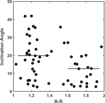
Figure 4. Centaur B – R colors and orbital inclination angles, i. The horizontal lines represent the median i of the gray and red populations. Application of the Wilcoxon rank sum test gives a 99.3% confidence level that red Centaurs have a smaller i distribution than gray Centaurs. Notice that only four red Centaurs have i values above the median i of the gray Centaurs. We are confident that red Centaurs have a smaller inclination angle distribution than gray Centaurs.
Download figure:
Standard image High-resolution imageTable 7. Number, Median, Stan Dev, Wilcoxon CL
| Param | nG |

|

|
nR |

|

|
CL (%) |
|---|---|---|---|---|---|---|---|
| i | 37 | 19.9 | 32.9 | 25 | 12.6 | 9.3 | 99.3 |
| a | 37 | 19.9 | 92.8 | 25 | 19.9 | 102.1 | 31 |
| e | 37 | 0.37 | 0.22 | 25 | 0.38 | 0.20 | 5 |
| q | 37 | 12.0 | 4.5 | 25 | 11.8 | 5.7 | 43 |
| Albedo | 17 | 5.9 | 1.2 | 11 | 12 | 5.4 | 99.9 |
| H | 37 | 9.4 | 1.4 | 25 | 10.4 | 1.6 | 93 |
Download table as: ASCIITypeset image
In Figures 5–7, we plot B – R color versus a, e, and q, respectively. The horizontal lines represent the median values of a, e, and q for the gray and red Centaurs. In contrast with the inclination angles in Figure 4, the medians of the gray and red Centaurs for a, e, and q in these figures appear almost identical. Application of the Wilcoxon rank sum test finds that there is only a 31%, 5%, and 43% probability that red Centaurs have different values of a, e, and q than the gray Centaurs, respectively. In other words, we find no statistically significant difference between the a, e, and q values of gray and red Centaurs. The number of objects, medians, standard deviations, and confidence levels are given in Table 7. In Tegler et al. (2008), we found no evidence of the any difference in a, e, or q between the red and gray populations for the smaller sample size of 26 objects.

Figure 5. Centaur B – R colors and semimajor axes, a. The horizontal lines represent the median a values of the gray and red Centaurs. Application of the Wilcoxon rank sum test gives only a 31% confidence level that red and gray Centaurs have different a distributions. We see no evidence of a difference in the semimajor axis distributions of the gray and red Centaurs.
Download figure:
Standard image High-resolution image
Figure 6. Centaur B – R colors and eccentricities, e. The horizontal lines represent the median e values of the gray and red Centaurs. Application of the Wilcoxon rank sum test gives only a 5% confidence level that red and gray Centaurs have different e distributions. We see no evidence of a difference in the eccentricity distributions of the gray and red Centaurs.
Download figure:
Standard image High-resolution image
Figure 7. Centaur B – R colors and perihelion distances, q. The horizontal lines represent the median q values of the gray and red Centaurs. Application of the Wilcoxon rank sum test gives only a 43% confidence level that red and gray Centaurs have different q distributions. We see no evidence of a difference in the perihelion distance distributions of the gray and red Centaurs.
Download figure:
Standard image High-resolution imageIn Figure 8, we present B – R color versus albedo. The horizontal lines represent the median values of the gray and red Centaurs for albedo. Application of the Wilcoxon rank sum test finds that there is a 99.9% probability that the red Centaurs have a larger albedo than the gray Centaurs. Our sample size is limited to only 28 objects because our B – R measurements only overlap 28 albedo measurements of Centaurs by Stansberry et al. (2008) and Bauer et al. (2013). In Table 8, we present the B – R colors and albedos in Figure 8. The number of objects, medians, standard deviations, and confidence levels are given in Table 7. In Tegler et al. (2008), we found a 99% probability that the red Centaurs have larger albedos than the gray Centaurs using a sample of 15 objects. Our larger sample size reported here demonstrates that red Centaurs have a statistically significant larger albedo than gray Centaurs. In agreement with this result, Lacerda et al. (2014) found a sample of 109 KBOs cluster into two groups—red KBOs with larger albedos than gray KBOs with smaller albedos.

Figure 8. Centaur B – R colors and albedos. The horizontal lines represent the median albedo values of the gray and red Centaurs. Application of the Wilcoxon rank sum test gives a 99.9% confidence level that red Centaurs have larger albedos than gray Centaurs. We are confident that red Centaurs have larger albedos than gray Centaurs.
Download figure:
Standard image High-resolution imageTable 8. Centaur Colors and Albedos
| Number | Designation/Name | B – R | Albedo (%)a |
|---|---|---|---|
| 167P | CINEOS | 1.29 | 5.3 |
| 5145 | Pholus | 1.97 | 16.0 |
| 7066b | Nessus | 6.0 | |
| 8405 | Asbolus | 1.22 | 5.0 |
| 10199 | Chariklo | 1.25 | 7.5 |
| 10370 | Hylonome | 1.16 | 6.0 |
| 31824 | Elatus | 1.75 | 5.0 |
| 32532 | Thereus | 1.18 | 5.9 |
| 52872 | Okyrhoe | 1.21 | 5.8 |
| 52975 | Cyllarus | 1.72 | 12 |
| 54598 | Bienor | 1.15 | 5.0 |
| 55576 | Amycus | 1.82 | 18.0 |
| 60558 | Echeclus | 1.39 | 7.7 |
| 63252 | 2001 BL41 | 1.21 | 4.0 |
| 83982 | Crantor | 1.86 | 11.0 |
| 120061 | 2003 CO1 | 1.24 | 7.2 |
| 136204 | 2003 WL7 | 1.23 | 4.6 |
| 145486 | 2005 UJ438 | 1.64 | 21.5 |
| 248835 | 2006 SX368 | 1.22 | 4.6 |
| 250112 | 2002 KY14 | 1.75 | 18.5 |
| 281371 | 2008 FC76 | 1.60 | 12.0 |
| 309737 | 2008 SJ236 | 1.60 | 7.4 |
| 342842 | 2008 YB3 | 1.23 | 6.2 |
| 346889 | Rhiphonos | 1.37 | 6.2 |
| 382004 | 2010 RM64 | 1.56 | 15.9 |
| 2002 GZ32 | 1.03 | 5.3 | |
| 2007 VH305 | 1.18 | 7.0 | |
| 2010 TH | 1.19 | 7.8 |
Notes.
aBauer et al. (2013). bV–R color is red. See Tegler & Romanishin (1998).Download table as: ASCIITypeset image
In Figure 9, we plot B – R color versus absolute visual magnitude, HV. The horizontal lines represent the median values of HV for the gray and red Centaurs. Application of the Wilcoxon rank sum test finds p = 0.07 which shows an almost significant difference between HV values of red and gray Centaurs. The number of objects, medians, standard deviations, and confidence levels are given in Table 7. The red Centaurs have larger albedos than the gray Centaurs and so the possibly larger median HV for the red Centaurs suggests that red Centaurs may have smaller diameters than gray Centaurs.

Figure 9. Centaur B – R colors and absolute visual magnitude, HV. The horizontal lines represent the median HV values of the gray and red Centaurs. Application of the Wilcoxon rank sum test gives p = 0.07 which shows an almost significant difference between HV values of red and gray Centaurs. The red Centaurs have larger albedos than the gray Centaurs and so the possibly larger median HV for red Centaurs suggests that red Centaurs may have smaller diameters than gray Centaurs.
Download figure:
Standard image High-resolution image6. COLOR−MAGNITUDE DIAGRAM OF KBOS AND CENTAURS
By combining the 63 new B – R color measurements in Tables 3–6 with our previously published B – R colors, we extend our sample size to 148 KBOs and Centaurs. Our database has optical photometry for 154 objects; however, six objects do not have B-band measurements and so we have B – R colors for 148 objects. In Figure 10, we plot our B – R versus HV for these 148 objects. Different dynamical groups in Figure 10 are color-symbol coded as follows: Centaurs (cyan circles), classicals (red squares), Plutinos (yellow upward triangles), scattered objects (blue downward triangles), and non-Plutino resonant objects (green diamonds). Uncertainties (error bars) are assigned to each B – R measurement. In many cases the error bars are smaller than the symbols. Our median uncertainty in B – R is 0.04 magnitude. We do not assign uncertainties (error bars) to our HV measurements because the uncertainties are dominated by lightcurve effects and we have lightcurves for only a handful of objects in Figure 10. We take the values of HV as proxies for the diameters of the KBOs and Centaurs.

Figure 10. Absolute visual magnitudes, HV, vs. B – R colors for Centaur (cyan circles), classical (red squares), Plutino (yellow upward triangles), scattered (blue downward triangles), and non-Plutino resonant (green diamonds) objects. Objects with HV > 7.0 are bimodal at the 99.96% confidence level. Objects with HV < 6.0 are bimodal at the 96% confidence level. Objects with 6.0 ≤ HV ≤ 7.0 exhibit a continuum of colors.
Download figure:
Standard image High-resolution imageTwo patterns are apparent in Figure 10. First, objects with HV > 7.0 appear to exhibit two color populations. This group of objects is dominated by Centaurs (cyan circles) but includes a sizable number of classical objects (red squares). Application of the dip test to the 93 objects in our survey with HV > 7.0 regardless of dynamical class indicates that these objects exhibit two color populations at the 99.96% confidence level. Remember, we found the Centaurs in our survey were bimodal at the 81% confidence level. Second, objects with HV < 6.0 appear to exhibit two color populations. Application of the dip test to the 36 objects with HV < 6.0 in our survey regardless of dynamical class indicates these objects exhibit two color populations at the 96% confidence level.
Peixinho et al. (2012) found similar patterns from an examination of HR magnitudes and B – R colors for 253 objects in the literature. They applied the dip test to 124 objects with HR > 6.8 and found a 99.9% probability that the objects divide in two color groups. Their result is in good agreement with our result. We point out that the intrinsically faintest object in Peixinho et al. (2012) is the Centaur 1994 TA for which they report HR = 11.4. In our survey, we find 1994 TA has HV = 12.04. Six of the new observations reported here are about as intrinsically faint as 1994 TA or fainter than 1994 TA. 2013 UL10 is our intrinsically faintest object and it is almost 1.5 magnitudes fainter than 1994 TA. The DCT is allowing us to measure some of the intrinsically faintest Centaurs known. For the intrinsically brightest objects, Peixinho et al. (2012) found strong evidence for bimodality for objects with HR < 5.6. Again, their result is in good agreement with our result.
The "H" pattern in Figure 10 is suggestive of bimodal colors for all 148 objects in our survey. Application of the dip test to our 148 KBO and Centaur B – R colors gives a p-value of 0.006, i.e., our entire sample of objects is bimodal at the 99.4% confidence level. In Figure 11, we show a B – R histogram for the 148 objects, and the best fit GMM model. We note that our original paper on the bimodality of KBO and Centaur colors only had 13 objects (Tegler & Romanishin 1998). Application of the dip test to our original sample of 13 objects indicates KBOs and Centaur colors are bimodal at the 99.4% confidence level.

Figure 11. B – R histogram of 148 Centaurs and KBOs. Application of a GMM decomposes our sample into two normal distributions, one with mean B – R = 1.22 and σ = 0.13, and the other with mean B – R = 1.69 and σ = 0.13. Application of the dip test to the sample gives a p-value of 0.006, i.e., a  confidence in bimodality.
Download figure:
Standard image High-resolution image
7. DISCUSSION
Our measurements constitute a unique data set. In particular, the median uncertainty in our B – R colors is 0.04 magnitude whereas the median uncertainty reported in the literature is 0.08 magnitude (Peixinho et al. 2012, 2015).
An interesting result reported here is that the red Centaurs exhibit a lower inclination angle distribution than gray Centaurs. This is the second correlation between the color of a KBO or Centaur and an orbital property. We first reported that cold classical KBOs are dominated by red colors (Tegler & Romanishin 2000) 16 years ago. We point out that the number of Centaurs in our survey with B – R colors is almost twice the number available in the literature (Peixinho et al. 2015).
The second interesting result reported here is the confirmation of work done by Peixinho et al. (2012) that intrinsically faint (small) objects and intrinsically bright (large) objects exhibit bimodal colors. See Figure 10 in this paper. Unlike Peixinho et al. (2012), we find our entire sample of colors exhibits bimodal colors.
More observations of HV and B – R are essential to flush out any additional patterns in Figure 10. Does the bimodal color pattern for intrinsically faint (small) objects extend to even intrinsically fainter (smaller) objects? Do intrinsically faint (small) Plutinos and scattered disk objects exhibit bimodal colors? Is there a dearth of objects in the color−magnitude diagram at B – R ∼ 1.7 and HV ∼ 6? Is bimodality related to object size or dynamical class? Bigger sample sizes are essential to answer these questions.
Patterns in the color−magnitude diagram of Figure 10 could provide an observational anchor for better understanding the formation and evolution of KBOs and Centaurs. Perhaps patterns in Figure 10 and theoretical models could help constrain the relative importance of primordial versus evolutionary processes on KBOs and Centaurs. Could color−magnitude diagrams of KBOs and Centaurs be as important to planetary evolution as color−magnitude diagrams of stars are to stellar evolution? Again, bigger sample sizes are essential to find out.
We are grateful to the NASA Solar System Observations Program for support, NAU for joining the Discovery Channel Telescope Partnership, and the Vatican Observatory for the consistent allocation of telescope time over the last 12 years of this project. These results made use of Lowell Observatory's Discovery Channel Telescope. Lowell operates the DCT in partnership with Boston University, Northern Arizona University, the University of Maryland, and the University of Toledo. Partial support of the DCT was provided by Discovery Communications. LMI was built by Lowell Observatory using funds from the National Science Foundation (AST-1005313).