


ABSTRACT
Light curves of 26 probable contact binary stars are made available, from a list of candidates with the shortest periods known. This is supplemented by sets of light curves of three previously studied systems. Photometry was obtained in the Johnson UBV, Cousins RI system. All stars but one were observed in four wavebands, either UBV RC or  , depending on brightness. Tentative spectral classifications are given for 23 of the stars. Effective temperatures are derived from infrared and optical photometric indices, and from spectral types. These are generally in good agreement. The multicolor photometry, spectral typing, and estimated effective temperatures can be used to model these systems in detail. A preliminary study, based on Fourier coefficients of the light curves, suggests that all the systems are indeed eclipsing stars, with all but a handful probably in contact configurations.
Export citation and abstract BibTeX RIS
1. INTRODUCTION
W Uma stars are short period (generally a few hours) eclipsing binary stars. The components are main-sequence stars of spectral types F to K, which are in thermal contact, so that their effective temperatures differ very little (e.g., Van Hamme & Cohen 2008). Despite this, the masses of the two components may be rather different. Light curves are continuously variable due to tidal deformation of the two stars. The two eclipse depths usually differ little (e.g., Paczyński et al. 2006), and color indices do not vary much over the binary cycle (Webbink 2003). As a rule eclipse depths vary little with the wavelength of observation. For the short period cooler stars discussed in this paper, the W Uma systems are of W type, in which the primary minimum results from occultation of the less massive star by the more massive primary.
There is a fairly sharp lower limit of about 0.2 days to the period distribution of contact binaries (e.g., Paczyński et al. 2006). Recent explanations for this phenomenon have been published by Jiang et al. (2012) and Stȩpień & Gazeas (2012), where references to earlier work can be found. The models of Stȩpień & Gazeas (2012), in particular, predict a minimum period close to 0.20 day. It is therefore of some interest to determine the true nature of candidate contact binaries with periods near this limit, such as the stars which form the subject of this paper.
Until 2008 only two contact binary systems with periods below 0.23 day were known—CC Com (P = 0.2207 day; Wenzel 1967) and GSC 01387-00475 (P = 0.2178 day; Rucinski & Pribulla 2008). Since then the advent of large photometric surveys, in particular those designed to search for planetary transits, has led to the discovery of numerous candidate W UMa systems with very short periods. Examples include Becker et al. (2011; using the Sloan Digital Sky Survey); Coughlin et al. (2011; Kepler); Hartman et al. (2011; Hungarian Automated Telescope Network, HATNet); Norton et al. (2011; Super Wide Angle Search for Planets, SuperWASP); Birkby et al. (2012), Nefs et al. (2013), and Zendejas Dominguez et al. (2013; Wide Field Camera Transit Survey, WFCAM); and Palaversa et al. (2013; Lincoln Near-Earth Asteroid Research, LINEAR). This paper is concerned with multi-filter follow-up observations of such stars found by the SuperWASP collaboration (Pollacco et al. 2006)—see the list in Norton et al. (2011).
The SuperWASP project performs a search for extrasolar planets, by photometric monitoring of a very large number of stars over many years, in order to detect transit signals (Pollacco et al. 2006). Since the telescopes are modest, consisting of telephoto lenses, individual measurements have low accuracy. However, typically thousands of measurements per object have been obtained for more than 30 million targets (Smith & The WASP consortium 2014). This makes SuperWASP photometry a valuable resource for discovering large amplitude periodic variable stars such as contact binaries.
Norton et al. (2011) identified 53 candidate contact binary stars with periods shorter than 0.232 day among SuperWASP variables, and presented light curves and periods for these stars (although the periods of a few stars were later revised by Lohr et al. 2012). Five of the 53 Norton et al. (2011) stars were re-discoveries of known binaries. Individual studies of a further nine stars on their list have been published—see Table 1.
Table 1. Published Studies, Including Modeling, of Individual Very Short Period SuperWASP Contact Binaries from the List of Norton et al. (2011)
| Name | Period | References |
|---|---|---|
| (day) | ||
| ROTSE1 J170240.11+151122.7 | 0.23119 | Akerlof et al. (2000) |
| 1SWASP 150822.80–054236.9 | 0.23006 | Lohr et al. (2014) |
| ASAS J111932–3950.8 | 0.22949 | Pojmański (2003) |
| 1SWASP 210318.76+021002.2 | 0.22859 | Elkhateeb et al. (2014a) |
| V1067 Her | 0.22853 | Blattler & Diethelm (2001) |
| V1104 Her | 0.22788 | Liu et al. (2015b) |
| 1SWASP 160156.04+202821.6 | 0.22653 | Lohr et al. (2014); Essam et al. (2014) |
| 1SWASP 074658.62+224448.5 | 0.22085 | Jiang et al. (2015) |
| 1SWASP 055416.99+442534.1 | 0.21825 | Dimitrov & Kjurkchieva (2015) |
| 1SWASP 133105.91+121538.0 | 0.21801 | Elkhateeb et al. (2014b) |
| 1SWASP 080150.03+471433.8 | 0.21751 | Dimitrov & Kjurkchieva (2015) |
| 1SWASP 234401.81–230232.3 | 0.21367 | Lohr et al. (2013); Koen (2014) |
| 1SWASP 022727.03+115641.7 | 0.21095 | Liu et al. (2015a) |
| BX Tri | 0.19264 | Dimitrov & Kjurkchieva (2010) |
Note. More commonly used names, rather than SuperWASP designations, are given for the five stars known prior to rediscovery by SuperWASP. Among these, binary models have only been fitted to observations of V1104 Her and BX Tri.
Download table as: ASCIITypeset image
This paper presents light curves, color indices, and, in most cases, spectral classifications for a further 26 stars from the Norton et al. (2011) list. Effective temperatures of the binary systems are derived from these data. The information can be exploited to evaluate whether candidates are truly contact systems, and to model the binaries in order to derive physical properties such as mass ratios and overfilling factors, etc. As mentioned above, the temperatures of the two components differ little, so that accurately determined values should be useful in constraining physical models.
The idea has been advanced in the literature that most, if not all, contact binaries are in triple or higher order systems (Paczyński et al. 2006; Pribulla & Rucinski 2006). The presence of a companion could be important in explaining the formation of contact binaries. One of the additional benefits derived from detailed modeling is to test for third light in these systems. Full models of the binary systems will also allow examination of correlations of component masses or component radii with binary periods—see the brief discussion in Norton et al. (2011).
New observations of three previously published systems (1SWASP 210318.76+021002.2, 1SWASP 160156.04+202821.6, and 1SWASP 022727.03+115641.7) are also provided in this paper; this allows the long-term repeatability of light curves to evaluated. Although the full stellar designations will be used in the tables, for convenience names will be abbreviated in the text.
2. OBSERVATIONS
Most photometric measurements were made with the South African Astronomical Observatory (SAAO) STE4 CCD camera mounted on the SAAO 1.0 m telescope at Sutherland, South Africa. The field of view of the camera on the telescope is 5 × 5 arcmin2. Pre-binning of the images was performed throughout, giving a reasonable readout time of about 17 s. The filters used were Johnson UBV and Cousins  (but for convenience the subscript C will be omitted below). Observations were cycled through either UBVR (for the brighter stars) or BVRI—see Table 2 for an observing log. One star—2MASS 1156–0912—was observed in BVR only. For each star, exposure times were tailored both to changing atmospheric conditions (seeing and cloud cover) and to the specific filter, ranging from 5–45 s (I), 5–60 s (R), 10–90 s (V), 16–160 s (B), and 120–160 s (U). The aim was to obtain peak count rates of 5000–10,000 per pixel. Run lengths were designed to cover one full binary orbit (i.e., typically 5.0–5.5 hr); in a few cases multiple (2–4) runs were required for complete phase coverage. Most of the observations were made under photometric, or mildly non-photometric, weather conditions. Notable exceptions are the first run on SWASP 0040+0716 and observations of SWASP 1219–2400 (extinctions of 0.1–0.2 mag), SWASP 0927–3911 (several times 0.1 mag extinction), and SWASP 1201–2201 (up to ∼1 mag of extinction). In Table 2 there are generally small differences between the numbers of observations through the different filters. This is because of the elimination of a few obviously discrepant measurements from light curves, typically due to adverse weather conditions.
Table 2. The Observing Log
| Name | Period | Start HJD | NU | NB | NV | NR | NI | Spectroscopic Grating |
|---|---|---|---|---|---|---|---|---|
| (day) | (2450000+) | |||||||
| 1SWASP J000437.82+033301.2 | 0.26150 | 6881.4959 | 0 | 0 | 56 | 57 | 58 | 7 |
| 7326.2495 | 0 | 51 | 50 | 53 | 50 | |||
| 1SWASP J155822.10–025604.8 | 0.26008 | 7270.2159 | 0 | 27 | 28 | 28 | 25 | 7 |
| 7271.2138 | 0 | 34 | 34 | 36 | 33 | |||
| 7272.2094 | 0 | 33 | 33 | 33 | 33 | |||
| 1SWASP J173828.46+111150.2 | 0.24938 | 6882.2073 | 0 | 70 | 73 | 72 | 72 | 6, 7 |
| 1SWASP J195900.31–252723.1 | 0.23814 | 6881.2449 | 0 | 60 | 76 | 76 | 68 | 6 |
| 1SWASP J052036.84+030402.1 | 0.23140 | 7017.3019 | 49 | 55 | 55 | 54 | 0 | 6 |
| 1SWASP J041655.13–492709.8 | 0.23102 | 7014.2863 | 0 | 54 | 52 | 54 | 55 | 7 |
| 1SWASP J051501.18–021948.7 | 0.23090 | 7015.3814 | 0 | 30 | 31 | 31 | 31 | 7 |
| 7019.4125 | 0 | 18 | 20 | 20 | 20 | |||
| 2MASS J23261012–2941470 | 0.23012 | 7274.3865 | 0 | 88 | 88 | 86 | 91 | 6, 7 |
| 1SWASP J034439.97+030425.5 | 0.22988 | 7011.3049 | 0 | 33 | 48 | 48 | 51 | 7 |
| 7329.3952 | 39 | 47 | 47 | 47 | ||||
| 2MASS J16133577–2847225 | 0.22978 | 6877.2436 | 0 | 91 | 97 | 96 | 95 | 7 |
| 1SWASP J050904.45–074144.4 | 0.22958 | 7016.2933 | 58 | 59 | 59 | 59 | 0 | 7 |
| 1SWASP J004050.63+071613.9 | 0.22927 | 6878.4927 | 0 | 106 | 110 | 108 | 108 | 6, 7 |
| 7277.5278 | 0 | 0 | 30 | 31 | 30 | |||
| 7279.5110 | 0 | 0 | 34 | 36 | 36 | |||
| 7281.4970 | 0 | 66 | 68 | 67 | 67 | |||
| 2MASS J21031997+0209339 | 0.22859 | 7277.2506 | 0 | 44 | 47 | 45 | 45 | 7 |
| 1SWASP J212454.61+203030.8 | 0.22783 | 7271.3593 | 0 | 59 | 59 | 59 | 59 | ⋯ |
| 1SWASP J114929.22–423049.0 | 0.22731 | 6758.2649 | 0 | 91 | 92 | 91 | 91 | 6 |
| 1SWASP J120110.98–220210.8 | 0.22717 | 6766.2310 | 0 | 67 | 103 | 71 | 75 | ⋯ |
| 1SWASP J030749.87–365201.7 | 0.22667 | 7010.3021 | 0 | 49 | 52 | 56 | 56 | 7 |
| 1SWASP J160156.04+202821.6 | 0.22653 | 7268.2273 | 0 | 37 | 38 | 38 | 38 | ⋯ |
| 7274.2169 | 0 | 33 | 33 | 32 | 32 | |||
| 1SWASP J121906.35–240056.9 | 0.22637 | 6768.2481 | 0 | 60 | 61 | 61 | 60 | ⋯ |
| 2MASS J09275494–3910527 | 0.22534 | 6765.2150 | 45 | 47 | 46 | 46 | 0 | ⋯ |
| 1SWASP J212808.86+151622.0 | 0.22484 | 7272.3358 | 0 | 41 | 44 | 45 | 40 | 6, 7 |
| 7274.3352 | 0 | 12 | 12 | 12 | 12 | |||
| 7281.2933 | 0 | 29 | 30 | 31 | 30 | |||
| 1SWASP J040615.79–425002.3 | 0.22234 | 7013.2962 | 0 | 49 | 54 | 56 | 60 | 6 |
| 1SWASP J224747.20–351849.3 | 0.21822 | 7279.2581 | 0 | 68 | 68 | 69 | 69 | 6, 7 |
| 2MASS J04112059–2302332 | 0.21632 | 7012.2889 | 0 | 74 | 74 | 75 | 75 | 7 |
| 2MASS J02272637+1156494 | 0.21095 | 7009.2978 | 0 | 40 | 41 | 41 | 42 | 7 |
| 2MASS J11560563–0912573 | 0.21091 | 6764.2440 | 0 | 69 | 85 | 87 | 0 | 6 |
| 2MASS J15165453+0048263 | 0.21073 | 6768.4826 | 41 | 52 | 52 | 53 | 0 | ⋯ |
| 1SWASP J142312.63–222425.1 | 0.20964 | 6757.4563 | 0 | 97 | 95 | 92 | 92 | 6 |
| 2MASS J21042404+0731381 | 0.20909 | 7270.3332 | 0 | 66 | 68 | 67 | 66 | 6, 7 |
Note. Most photometric runs covered approximately one binary period. The filter system used was Johnson UBV and Cousins RI. Periods of the binaries, given in Column 2, were taken from Norton et al. (2011), except for the first four stars which have corrected periods from Lohr et al. (2012). Columns 5–8 shows the number of usable measurements obtained in each of the UBVRI filters. The last column indicates the grating used to obtain spectra of 23 of the stars: grating 6 covers ∼3600–5400 Å at 2 Å resolution, grating 7 covers ∼3600–7500 Å at 5 Å resolution.
Download table as: ASCIITypeset image
Reductions were performed using an automated version of DOPHOT (Schechter et al. 1993). Magnitudes determined from point-spread function fitting were preferred over aperture photometry, since the noise levels of the light curves were found to be lower.
Differential magnitudes of the stars, calculated with respect to bright local comparison stars in the field of view, are supplied as online material supplementary to this paper. All light curves are made available in a single file with five colums,namely object name; filtername; Heliocentric Julian Day (HJD) of observation; fractional HJD; and differential magnitude (adjusted to zero mean). In some cases (particularly for stars observed on multiple nights) the third column is replaced by zeros and the fourth by phase. Example light curves for a bright star are plotted in Figure 1.
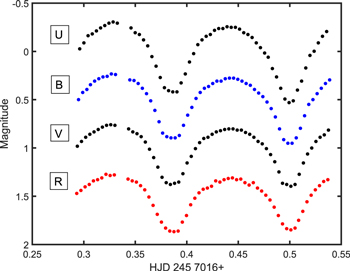
Figure 1. Light curves of SWASP 0509–0741 (P = 0.22958 day). Magnitude zeropoints are arbitrary. The estimated average errors for the UBVR light curves are, respectively, 0.015, 0.012, 0.011, and 0.012 mag. Errorbar sizes are therefore similar to the plotting point sizes in the figure. Note the pronounced O'Connell effect (e.g., Davidge & Milone 1984) in U, and the change in relative eclipse depths with wavelength. The data behind this figure include both these light curves and light curves for all other stars, and are provided in machine readable format.(The data used to create this figure are available.)
Download figure:
Standard image High-resolution imageExposure times were chosen to give peak count rates of a few thousands counts per pixel for the program stars. The actual numbers obtained usually varied substantially due to changes in observing conditions.
Typical measurement errors σe were estimated from the final differentially corrected light curves using the method of Gasser et al. (1986; see also Dette et al. 1998). For all but nine of the 115 data sets  mag. All three sets of observations of 2MASS 1156–0912 are among those with
  , with
  mag for the B filter the only error in excess of 0.04 mag among the 115 data sets. Due to poor seeing conditions, images of this star were partially blended with those of 2MASS J115605.88–0913007, 5 arcsec distant, and 1.3 mag brighter than the target star in the DENIS I band (Epchtein et al. 1999).
If the "signal" S is defined to be half the amplitude of peak to peak variation, then the minimum signal-to-noise ratio (S/N) over all data sets is  , for the B filter observations of the low amplitude (
 mag) star SWASP 1423–2224. Other S/N are in the range 5.8–49.
The SuperWASP CCD scale is 13.7 arcsec per pixel (Pollacco et al. 2006), so it is surprising that so few of the coordinates assigned to variables are ambiguous or in error. Table 3 contains corrected positions for nine of the variables.
Table 3. Corrected Positions for Nine of the Short Period Contact Binary Candidates
| SuperWASP Name | 2MASS Name |
|---|---|
| 1SWASP J022727.03+115641.7 | 2MASS J02272637+1156494 |
| 1SWASP J041120.40–230232.3 | 2MASS J04112059–2302332 |
| 1SWASP J092756.25–391119.2 | 2MASS J09275494–3910527 |
| 1SWASP J115605.88–091300.5 | 2MASS J11560563–0912573 |
| 1SWASP J151652.90+004835.8 | 2MASS J15165453+0048263 |
| 1SWASP J161334.28–284706.7 | 2MASS J16133577–2847225 |
| 1SWASP J210318.76+021002.2 | 2MASS J21031997+0209339 |
| 1SWASP J210423.76+073140.4 | 2MASS J21042404+0731381 |
| 1SWASP J232607.07–294130.7 | 2MASS J23261012–2941470 |
Note. The SuperWASP names are from Table 1 in Norton et al. (2011), while the 2MASS names were obtained by matching the observed positions (in the SAAO photometry) of the variables to the closest 2MASS star position.
Download table as: ASCIITypeset image
Additionally, standardized photoelectric photometry of three program stars, and the related star 1SWASP J234401.81–212229.1 (hereafter SWASP 2344–2122), was obtained with the Modular Photometer on the SAAO 0.5 m telescope. Conditions were photometric on the two nights during which observations were made. Each star was measured twice, so that crude estimates of the photometric errors could be made. These are generally quite large: since the stars are relatively faint for the instrument/telescope combination, long integration times were needed. Since there is no autoguiding on the telescope, large apertures (20–30 arcsec) were required to avoid stars drifting too close to the aperture edge; even though all measurements were made under dark sky conditions, the sky background contribution was therefore non-negligible, with deleterious consequences for accuracy. Furthermore, since all four stars are quite red, U-band measurements were only possible for the two brightest objects. Results are in Table 4.
Table 4. Standardized Photoelectric Johnson UBV, Cousins RI Photometry of Four SuperWASP Binary Stars
| Name | V |

|

|

|

|
|---|---|---|---|---|---|
| SWASP 2344–2122 | 11.67 (0.02) | 1.15 (0.02) | 1.06 (0.05) | 0.68 (0.01) | 1.30 (0.01) |
| SWASP 0040+0716 | 12.18 (0.01) | 0.72 (0.01) | 0.14 (0.02) | 0.42 (0.01) | 0.88 (0.02) |
| SWASP 1149–4230 | 14.33 (0.07) | 1.23 (0.23) | ⋯ | 0.85 (0.01) | 1.66 (0.02) |
| SWASP 1201–2202 | 15.01 (0.03) | 1.12 (0.03) | ⋯ | 0.69 (0.05) | 1.29 (0.05) |
Note. Crude error estimates are given in brackets.
Download table as: ASCIITypeset image
Spectra were obtained for all but six of the 29 photometric targets. Spectroscopic observations were made with the SAAO SpCCD grating spectrograph, attached to the SAAO 1.9 m telescope. All the objects were observed with one or more 15 minute exposures, and were preceded and followed by calibration arc exposures. Two different gratings were used: number 6, with approximate wavelength coverage 3600–5600 Å at a resolution of 2 Å; and grating 7, covering roughly 3600–7500 Å at 5 Å resolution. Spectra were obtained in bright moonlight. Typical S/N for the grating 6 spectra range from 7 to 37 (mean 20), whereas the grating 7 spectra range from S/N 6 to 51 (mean 23).
Since no MK standard stars were observed on the same equipment, the spectra from both gratings were classified visually on the computer screen against the flux-calibrated standard star library libnor36 defined in Gray & Corbally (2014)4 . A list of the standard stars employed in that library may also be found on that same website. Neither the grating 6 nor the grating 7 spectra have the same resolution of the libnor36 standard spectra, and so some pre-processing was necessary before classification could be carried out. The spectral resolution of the grating 7 spectra were sufficiently similar to spectra in the standard library that only slight smoothing of the standard library spectra was required. However, for grating 6, the program spectra have a higher resolution than the standard library, and so the program spectra were smoothed and rebinned to the resolution of the standard library (∼3.6 Å).
The program spectra were not flux calibrated. The need to classify spectra that have not been flux calibrated is a common problem that may be overcome by a combination of two methods. First, most MK spectral criteria involve the estimation of line or band ratios of features that are closely adjacent in the spectrum (see Gray & Corbally 2009), meaning that accurate flux calibration is not essential for spectral classification. Second, a method of "flux correction" has been developed to deal with this problem in the context of automatic classification (see Gray & Corbally 2014). This is an iterative process. The classifier (or classification program) first makes a rough classification of the uncalibrated spectrum based on MK spectral classification line-ratio criteria. This rough spectral type is then used to select a flux-calibrated standard spectrum from the standards library to use as a flux "template." The continuum of the program spectrum is then "adjusted" to that of the standard spectrum, and a new spectral type is derived based on this "flux corrected" spectrum. That revised spectral type is used to select a new flux template, and the process is iterated to convergence. Usually this flux correction process results in only minor changes to the original "rough" spectral type, but it can be important in deriving precise types.
The resulting spectral types ranged from early G- through mid K-types, and so the MK criteria employed were appropriate for those spectral types. A detailed discussion of those spectral criteria may be found in Gray & Corbally (2009).
Some of the program spectra were very noisy, which resulted in some very uncertain types, indicated with a colon (:) in Table 5.
Table 5. Photometric Indices and Spectral Types of the Stars
| Name | APASS B − V | SAAO B − V | V − R | V − I | AV | Spectral Type |
|---|---|---|---|---|---|---|
| (mag) | (mag) | (mag) | (mag) | (mag) | ||
| 1SWASP J000437.82+033301.2 | ⋯ | 0.813 | 0.431 | 0.792 | 0.048 | G5 |
| 1SWASP J155822.10–025604.8 | ⋯ | 1.221 | 0.691 | 1.383 | 0.998 | K0: |
| 1SWASP J173828.46+111150.2 | ⋯ | 1.110 | 0.626 | 1.199 | 0.477 | K0–K2.5 |
| 1SWASP J195900.31–252723.1 | ⋯ | 0.946 | 0.551 | 1.074 | 0.381 | K2: |
| 1SWASP J052036.84+030402.1 | 0.890(0.033) | 0.990 | 0.539 | ⋯ | 0.330 | K0 |
| 1SWASP J041655.13–492709.8 | 1.034(0.027) | 1.045 | 0.602 | 1.172 | 0.040 | K0–K4: |
| 1SWASP J051501.18–021948.7 | ⋯ | 1.174 | 0.624 | 1.217 | 0.503 | K2: |
| 2MASS J23261012–2941470 | 1.022(0.051) | 1.041 | 0.655 | 1.121 | 0.065 | K3–K5 |
| 1SWASP J034439.97+030425.5 | 0.969(0.026) | 1.054 | 0.600 | 1.194 | 0.604 | G9 |
| 2MASS J16133577–2847225 | 1.250(0.047) | 1.312 | 0.824 | 1.649 | 0.577 | K7: |
| 1SWASP J050904.45–074144.4 | 0.986(0.034) | 1.050 | 0.588 | ⋯ | 0.247 | G9 |
| 1SWASP J004050.63+071613.9 | 0.725(0.088) | 0.871 | 0.453 | 0.877 | 0.108 | G1–G2 |
| 2MASS J21031997+0209339 | 0.658(0.112) | 1.219 | 0.922 | 1.740 | 0.246 | K5: |
| 1SWASP J212454.61+203030.8 | ⋯ | 1.162 | 0.633 | 1.240 | 0.318 | ⋯ |
| 1SWASP J114929.22–423049.0 | 1.434(0.054) | 1.389 | 0.841 | 1.641 | 0.494 | K0: |
| 1SWASP J120110.98–220210.8 | 1.131(0.048) | 1.190 | 0.494 | 1.047 | 0.135 | ⋯ |
| 1SWASP J030749.87–365201.7 | 1.024(0.075) | 1.097 | 0.643 | 1.255 | 0.059 | K3: |
| 1SWASP J160156.04+202821.6 | 1.204(0.074) | 1.316 | 0.799 | 1.492 | 0.151 | ⋯ |
| 1SWASP J121906.35–240056.9 | 1.153(0.112) | 1.108 | 0.633 | 1.214 | 0.270 | ⋯ |
| 2MASS J09275494–3910527 | 1.064(0.024) | 1.030 | 0.676 | ⋯ | 0.867 | ⋯ |
| 1SWASP J212808.86+151622.0 | ⋯ | 1.284 | 0.681 | 1.345 | 0.226 | K3–K5 |
| 1SWASP J040615.79–425002.3 | 0.987(0.047) | 0.976 | 0.562 | 1.074 | 0.028 | K2 |
| 1SWASP J224747.20–351849.3 | 1.190(0.023) | 1.411 | 0.857 | 1.656 | 0.040 | K4–K5 |
| 2MASS J04112059–2302332 | 1.288(0.080) | 1.178 | 0.698 | 1.342 | 0.121 | K5: |
| 2MASS J02272637+1156494 | ⋯ | 1.419 | 0.866 | 1.736 | 0.348 | M0: |
| 2MASS J11560563–0912573 | 0.693(0.039) | 1.255 | 0.765 | ⋯ | 0.096 | K3 |
| 2MASS J15165453+0048263 | 0.645(0.043) | 1.219 | 0.736 | ⋯ | 0.136 | ⋯ |
| 1SWASP J142312.63–222425.1 | 0.696(0.020) | 0.797 | 0.400 | 0.772 | 0.314 | G0 |
| 2MASS J21042404+0731381 | 0.625(0.116) | 1.237 | 0.719 | 1.422 | 0.195 | K2–K5 |
Note. The  indices in Column 2 are from Terrell (2014), as extracted from the AAVSO Photometric All-Sky Survey (APASS). Photometric indices in Columns 3–5 were estimated as described in Section 3. Dust absorption, retrieved from the NASA/IPAC extragalactic database, is listed in Column 6. Colons following spectral types in Column 7 indicate uncertain classifications.
Download table as: ASCIITypeset image
3. PHOTOMETRIC CALIBRATIONS
Because the focus was on obtaining light curves, which was possible even under very poor conditions by differentially correcting measurements, no standard stars were observed. Instead, use is made of several nights of photometry of the star SWASP 2344–2122, as described by Koen (2014). Those measurements were made with the same experimental setup (telescope, CCD camera, and filters), and hence can be used to derive accurate mean instrumental system colors. Furthermore, standard system photometry of SWASP 2344–2122 is listed in Table 4. The spectral class of the star is K5V (Lohr et al. 2013); the expected photometric indices are  ,
,  ,
,  , and
, and  (Pecaut & Mamajek 2013). The agreement of the Table 4 values with these is unexpectedly good.
Combining the standardized and instrumental system measurements provides the transformation equations
Note that SWASP 2344–2122 is of spectral type similar to that expected for the subjects of this paper, so that color effects should be small for the present application.
The estimated  ,
,  , and
, and  indices of the 29 program stars, as derived from the averaged light curves, are in Table 5. For the three stars in common with Table 4, agreement is reasonable, particularly for the only Table 4 star (SWASP 1149–4230) for which the CCD photometry was acquired under photometric conditions. In what follows, the photoelectric photometry is preferred for calibration, except for the very uncertain
  index of SWASP 1149–4230, for which the estimated
  is retained.
The number of measurements per filter for most of the stars is greater than 50. Given furthermore that the typical errors on individual measurements are only a few percent, the mean magnitudes, and hence instrumental colors, are very accurately determined. Most of the errors in the color indices in Table 5 should consequently be due to the relatively crude standardization in Equation (1). Checks for consistency of the indices with other available information (photometric indices from other sources, and spectral classifications) are made below.
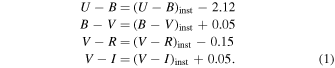
The AAVSO Photometric All-Sky Survey (APASS, see, e.g., Henden & Munari 2014) is a freely available source of BVgri photometry for millions of stars across the entire sky. Photometry for all the stars in Table 1 was extracted from this database. APASS photometric errors in  are available for all but two of the stars in Table 1, but are unfortunately generally quite large, ranging from 0.02 to 0.54 mag, with a mean of 0.21 mag. Table 5 lists
  indices extracted by Terrell (2014) from the APASS, for stars with at least two nights of observation. The agreement between the two sets of indices is reasonable, except, of course, for the mis-identified stars as listed in Table 3 (see Figure 2). There is a small systematic difference visible. There are at least two reasons why this is not unexpected. First, standardization of the APASS photometry is done with respect to Landolt standard stars (e.g., Munari et al. 2014). It is known that there are systematic differences between
  indices measured with respect to Landolt standard stars, and those determined using E-region standards in use at SAAO (e.g., Menzies et al. 1991). For stars with
  indices in the range covered in Table 5 the difference is in the sense that SAAO indices are of the order of 0.01–0.02 mag redder than Landolt system values. Second, APASS magnitudes are determined by aperture photometry. With aperture sizes of 15–20 arcsec (https://www.aavso.org/apass) it is inevitable that at least some light from faint nearby stars will be included in the photometry of some of the brighter targets. Obvious instances in the present case are 2MASS J02272637+1156494 (companions at ∼9 and ∼12 arcsec), and 2MASS J11560563–0912573 (companion ∼5 arcsec).
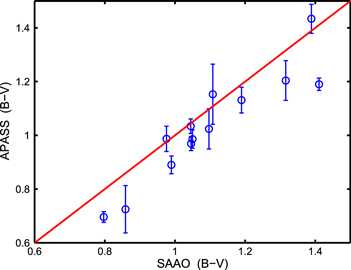
Figure 2. Comparison between the  indices estimated from the SAAO photometry, and those extracted from the APASS by Terrell (2014). Data are plotted only for those stars with correct SuperWASP coordinates.
Download figure:
Standard image High-resolution imagePhotometric indices were dereddened using the online NASA/IPAC Extragalactic Database, which is gratefully acknowledged. Two sets of reddening estimates, based, respectively, on the work of Schlegel et al. (1998) and Schafly & Finkbeiner (2011), are returned. The latter, more recent values are used in this paper. Using the alternative reddening estimates makes a difference of at most 200 K in the temperature estimated from the dereddened photometric indices, which amounts to at most one spectral subdivision. The estimated V-band absorption is given in column 6 of Table 5.
Figure 3 shows the dereddened color indices in Table 5 in color–color diagrams. Also shown are the color–color relations for main-sequence stars from Pecaut & Mamajek (2013). The fact that the observed indices lie close to the main-sequence line inspires some confidence in the calibration procedure. There is one outlying point in the top panel of Figure 3, corresponding to 2MASS 2103+0209. The dereddened  and
and  indices, respectively, indicate spectral types of K5 and K8; inspection of the light curves suggests the possible presence of a large starspot which may affect the colors—see also Elkhateeb et al. (2014b).
Figure 3. Two-color plots based on the dereddened indices from Table 5. Open circles denote CCD photometry, filled circles photoelectric photometry. The solid lines show the colors of main-sequence stars, according to Pecaut & Mamajek (2013). Arrows are reddening vectors for AV = 0.5 mag.
Download figure:
Standard image High-resolution imageThe scatter in diagrams involving the four  indices (not shown) is large, and these will not be used in what follows. Near-infrared (NIR) JHKS magnitudes of the stars were extracted from the Two Micron All Sky Survey (2MASS) point source catalog (Skrutskie et al. 2006). The mean quoted magnitude errors on all three filters are about 0.025 mag, maximum errors being 0.032, 0.037, and 0.033 mag for JHKS, respectively. These indices were also dereddened, as described above for the optical photometry. A two-color diagram based on these data can be seen in the top panel of Figure 4. The J magnitude of one star (SWASP 11560–0912) is clearly anomalously faint. The bottom panel of Figure 4 is constructed from one optical and one NIR index, and shows that the results for the two wavelength regimes are consistent.
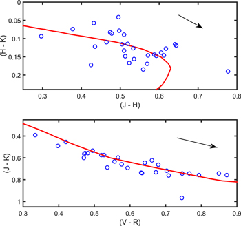
Figure 4. Top panel: two-color plot based on dereddened 2MASS photometry of the stars. Bottom panel: two-color plot demonstrating consistency of the optical and infrared indices. The mean errors in the 2MASS photometry of the stars are 0.025, 0.026, and 0.025 mag, respectively, for JHK. The solid lines show the colors of main-sequence stars, according to Pecaut & Mamajek (2013). Arrows are reddening vectors for AV = 0.5 mag.
Download figure:
Standard image High-resolution imageAs a consistency check spectral types derived from the optical photometric indices can be compared to the spectroscopic classifications in Table 5. The agreement is generally within two or three subtypes. The following are notable exceptions.
- i.SWASP 1149–4230 (K6 versus K0:). The spectrum was very noisy, and the classification therefore very uncertain.
- ii.SWASP 0040+0716 (G8 versus G1–G2). Inspection of light curves suggests that there might be a considerable third light contribution in the blue. Furthermore, the bluer the filters involved, the higher the implied temperature of the system—
 corresponds to G2, to G7.5, and to K1. The star is therefore probably a triple system, consisting of an early G star, together with a close binary comprising two late-type stars.
 - iii.SWASP 0509–0741 (K3 versus G9). All three photometric indices [including] imply a spectral type close to K3. Amplitudes of the light curves increase with decreasing wavelength, hinting at the presence of additional red light in the system. It is also worth noting that whereas primary and secondary eclipse depths are quite similar in R, they differ by ∼0.1 mag in U.


4. EFFECTIVE TEMPERATURES
Effective temperatures of the binaries were estimated from the dereddened optical photometric indices, again using the table provided by Pecaut & Mamajek (2013). This was done by minimizing (with respect to temperature) the sum of squared differences between observed and expected  ,
,  , and
, and  indices. Figure 5 compares the results to effective temperatures similarly derived from the dereddened 2MASS NIR indices, as a consistency check. The agreement is reasonable. Effective temperatures from the optical photometric indices are preferred, on the basis of the larger magnitude ranges in two-color diagrams, and the fact that generally three, rather than only two, indices are available for estimation. It is interesting that three of the largest discrepancies in Figure 5 are seen around temperatures near 5400 K (as estimated from optical indices). In two of these cases, spectra of the stars are available, and are more consistent with the higher optical-derived effective temperatures.
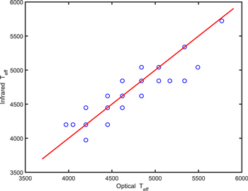
Figure 5. Effective temperatures derived, respectively, from the dereddened optical and infrared color indices. The line shows the locus of equal temperatures.
Download figure:
Standard image High-resolution imageAs an independent check it is noted that spectra of SWASP 1601+2028 were obtained by Lohr et al. (2014), and characterized by a temperature of 4500 K, in reasonable agreement with the entries in Table 6.
Table 6.
Effective Temperatures (in Degrees Kelvin) Estimated from Infrared Colors  and
and  Optical Indices
  , (
, ( , and
, and  and from the Spectroscopic Classifications of the Stars, Using Tabulations by Pecaut & Mamajek (2013)
| Name | T(infrared) | T(Optical) | T(Spectroscopic) |
|---|---|---|---|
| 1SWASP J000437.82+033301.2 | 5340 | 5340 | 5660 |
| 1SWASP J155822.10–025604.8 | 5040 | 5040 | 5280: |
| 1SWASP J173828.46+111150.2 | 4840 | 4840 | 4940–5280 |
| 1SWASP J195900.31-252723.1 | 4840 | 5170 | 5040: |
| 1SWASP J052036.84+030402.1 | 4840 | 5040 | 5280 |
| 1SWASP J041655.13–492709.8 | 4620 | 4620 | 4620–5280: |
| 1SWASP J051501.18–021948.7 | 4840 | 4840 | 5040: |
| 2MASS J23261012–2941470 | 4840 | 4840 | 4450–4840 |
| 1SWASP J034439.97+030425.5 | 4840 | 5040 | 5340 |
| 2MASS J16133577–2847225 | 4450 | 4450 | 4050: |
| 1SWASP J050904.45–074144.4 | 4620 | 4840 | 5340 |
| 1SWASP J004050.63+071613.9 | 5040 | 5490 | 5770–5880 |
| 2MASS J21031997+0209339 | 4200 | 4050 | 4450 |
| 1SWASP J212454.61+203030.8 | 5040 | 4840 | ⋯ |
| 1SWASP J114929.22–423049.0 | 4200 | 4200 | 5280: |
| 1SWASP J120110.98–220210.8 | 4840 | 4620 | ⋯ |
| 1SWASP J030749.87–365201.7 | 4450 | 4620 | 4840: |
| 1SWASP J160156.04+202821.6 | 4450 | 4200 | ⋯ |
| 1SWASP J121906.35–240056.9 | 4620 | 4840 | ⋯ |
| 2MASS J09275494–3910527 | 4840 | 5340 | ⋯ |
| 1SWASP J212808.86+151622.0 | 4200 | 4450 | 4450–4840 |
| 1SWASP J040615.79–425002.3 | 4620 | 4840 | 5040 |
| 1SWASP J224747.20–351849.3 | 4200 | 3970 | 4450–4620 |
| 2MASS J04112059–2302332 | 4200 | 4450 | 4450: |
| 2MASS J02272637+1156494 | 4200 | 4050 | 3850: |
| 2MASS J11560563–0912573 | 3970 | 4200 | 4840 |
| 2MASS J15165453+0048263 | 4200 | 4450 | ⋯ |
| 1SWASP J142312.63–222425.1 | 5720 | 5770 | 5920 |
| 2MASS J21042404+0731381 | 4620 | 4450 | 4450–5040 |
Download table as: ASCIITypeset image
Uncertainties in the estimated effective temperatures arise both from scatter around the Pecaut & Mamajek (2013) calibrations, and from photometric errors. Errors of the order of 0.02–0.04 in  will lead to uncertainties of a little more than 100 K at a typical spectral type of K0. The
  index is much more insensitive to temperature, hence similar errors translate to greater temperature uncertainties (several hundred degrees). Optical photometric indices are considerably more sensitive to temperature, and also more accurately determined, so that the temperature errors due to this source should be well below 100 K. The discussions in Pecaut & Mamajek (2013) suggest though that there could be considerable variation in reported effective temperatures at any given spectral type. This is not quantified in their paper. Absolute uncertainties in
  cannot therefore be provided, but differences between the three independent estimates in Table 6 should provide some insight into the level of consistency of the results.
5. DISCUSSION
It is not necessarily obvious from its light curves whether a given star is in a contact configuration. For example, slight differences in eclipse depths (as in Figure 1) may be indicative of a slight temperature difference between components, despite being in contact (e.g., Rucinski 1997a). Alternatively, such differences may be due to starspots.
It is possible to learn more about the nature of the stars by fitting truncated Fourier series
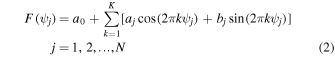
to the set of N observed fluxes in the light curve. In (2),  is the phase of the jth observation. The light curves are first normalized and shifted, so that maximum flux is unity, and zero phase is at the midpoint of primary minimum. We follow Pojmański (2002) in setting K = 4. As shown by Pojmański (2002; see also Rucinski 1997a, 1997b), the coefficients a2 and a4 can be used to discriminate between the light curves of contact and detached binaries. Furthermore, combinations of a4 and b4, or b2 and b4, are useful for telling eclipsing and pulsating variables apart.
Fourier coefficients a4 and b4, for each of the 115 light curves, are plotted in the top panel of Figure 6. One-sigma errors, calculated from the least squares parameter covariance matrix, are also shown. As demonstrated in Pojmanski (2002) (Figure 5(b)), eclipsing binary coefficients form a fairly narrow sequence parallel to the a4 axis and centered on  , while the coefficients of pulsating variables lie along a diagonal stretching roughly between the points
  and
and  . The suggestion from the top panel of Figure 6 is that only the four isolated points lying below the horizontal sequence, all corresponding to SWASP 1558–0256, may indicate pulsation. However, the light curves of this particular star are only 75% complete, lacking one of the two maxima, and hence the coefficients are poorly constrained (as can also be seen from the large errorbars on the points). Furthermore, the spectral type (K0:) argues against star being a pulsator, particularly given the large (∼0.7mag) peak to peak amplitudes of the light curves. We conclude that it is likely that all the stars are indeed eclipsing variables.
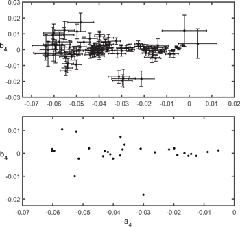
Figure 6. Fourier coefficients b4 and a4 of the light curves of the 29 stars (see Equation (2)). The top panel shows coefficient pairs for all 115 light curves, while the bottom panel displays averages for each of the 29 stars (excluding the shortest wavelength light curve).
Download figure:
Standard image High-resolution imageIn a number of cases the coefficient standard errors calculated from the U or B filter light curves are rather larger than the errors on the coefficients extracted from the other light curves. The bottom panel of Figure 6 show the mean values of the coefficients, calculated excluding data from the shortest wavelength filter.
Figure 7 is analogous to Figure 6, but is based on the coefficients (a2 and a4) most effective at discriminating between overcontact and detached binaries. The (red) line in the plots is the overcontact boundary
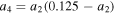
(Rucinski 1997a). Of the 29 systems, coefficients of one (SWASP 0040+0716) lies slightly below the limiting line, while a further six sets of coefficients are very close to the line (SWASP 1423–2224, SWASP 2124+2030, SWASP 1201–2202, SWASP 0416–4927, SWASP 0344+0304, and SWASP 2247–3518). Preliminary detailed modeling of the SWASP 1201–2202 light curves confirms that this star is probably not in an overcontact configuration.

Figure 7. As for Figure 6, but for the a2 and a4 coefficients. Points above the red line correspond to stars in overcontact configurations.
Download figure:
Standard image High-resolution image
6. CONCLUSIONS
As was pointed out in the Introduction, there is considerable interest in contact binary systems with periods of the order of 0.2 day. This paper presented photometry of 29 short period systems, taken from a list of candidates compiled by Norton et al. (2011). A preliminary analysis based on Fourier decomposition (Section 5) suggests that the greater majority of systems are indeed in overcontact configurations.
Light curves obtained in multiple wavebands (typically BVRI) are made available electronically for detailed modeling. This will be aided by effective temperatures derived from  and
and  indices. Reasonable agreement of the
  indices with those derived from APASS photometry, and good agreement of effective temperatures with those obtained from 2MASS JHK photometry, were demonstrated. Twenty-three of the stars were also classified spectroscopically. This supplementary information will aid modeling of the binary systems.
This paper has benefited from comments made by the referee. C.K. acknowledges funding from the South African National Research Foundation, and generous telescope time allocations by the South African Astronomical Observatory. Use of the Simbad database, Vizier catalog service, the 2MASS and DENIS point source catalogs, and the NASA/IPAC Extragalactic Database, is gratefully acknowledged.
Footnotes
- 4
Available for public download at http://www.appstate.edu/grayro/mkclass/.