DETECTION OF THE YORP EFFECT FOR SMALL ASTEROIDS IN THE KARIN CLUSTER

The Karin family with the estimated age of 5.75 ± 0.05 Myr is one of the youngest families in the main belt (Nesvorný et al. 2002; Nesvorný & Bottke 2004). Because of its recent formation, it is possible to numerically integrate the orbits backward in time and demonstrate the young age by showing that the orbits of individual members converge together at the time of the parent body breakup. Improving on previous work, Nesvorný & Bottke (2004) have shown that a precise reconstruction of the orbital histories requires that the Yarkovsky effect is taken into account in the backward integration. This allowed them to infer the semimajor axis drift rate for individual members of the Karin cluster and verify, for the first time, how the Yarkovsky effect operates on the main-belt asteroids over million-year-long timescales. A by-product of this study was a determination of spin obliquities for 70 individual members of the Karin cluster with absolute magnitudes $H\lt 16$ (roughly diameters $D\gt 2$ km for albedo ${p}_{{\rm{V}}}=0.2$).

Many new asteroids have been discovered since the last dynamical analysis of the Karin cluster. Here we repeat the analysis of Nesvorný & Bottke (2004) with an orbital catalog that contains nearly seven times more asteroids than there were available back in 2004. In Section 2, we revise the Karin family membership by applying the usual clustering method on the new orbital catalog. The taxonomical and albedo interlopers are eliminated. We then apply a more stringent criterion of the Karin family membership by requiring that orbits converged with each other $\simeq 5.75$ Myr ago. In Section 3, we use the method developed in Nesvorný & Bottke (2004) to estimate the Yarkovsky drift rates of individual bodies. This data is compared to the theoretical expectations for the Yarkovsky effect.

We find that the distribution of spin obliquities ε of small Karin members ($D\simeq 1\mbox{--}2$ km) is bimodal with only very few values near $\varepsilon =90^\circ$ and peaks for smaller and larger obliquities (Section 4). It is shown that this obliquity distribution is consistent with an initially random orientation of spin axes that was modified by the YORP effect (Sections 5–7; e.g., Rubincam 2000; Čapek & Vokrouhlický 2004). In Section 8, we apply a standard YORP model to estimate the thermal conductivity and calibrate the strength of the YORP effect. The results are discussed in Section 9. Finally, we perform new numerical simulations with the Yarkovsky force and/or gravitational perturbations of (1) Ceres (Section 10), and discuss the latter as a stochastic factor that sets firm limits on what can be achieved with this type of study. Section 11 presents our conclusions.

To define the Karin cluster membership, we first turned our attention to the family identification data from Nesvorný et al. (2015). In that work, the Karin cluster was identified using the Hierarchical Clustering Method (HCM hereafter) and a velocity cutoff of 10 m s⁻¹ in the domain of the proper orbital elements $(a,e,\mathrm{sin}i$; see Table 2 in Nesvorný et al. 2015 for further details). To eliminate possible interlopers, we adopted the classification scheme of DeMeo & Carry (2013). Specifically, we used the fourth release of the Sloan Digital Sky Survey-Moving Object Catalog (SDSS-MOC4; Ivezić et al. 2001) and computed the gri slope and $z^{\prime} -i^{\prime}$ colors. In addition, we used information from three major photometric/spectroscopic surveys: the Eight-color Asteroid Survey (Zellner et al. 1985; Tholen 1989), the Small Main Belt Spectroscopic Survey (Xu et al. 1995; Bus & Binzel 2002a, 2002b), and the Small Solar System Objects Spectroscopic Survey (Lazzaro et al. 2004). There were 13 objects with known taxonomical information in total, six of which have a C-complex taxonomy and are therefore incompatible with the S-type taxonomy of the Karin cluster. After eliminating these objects, we end up with a sample of 535 Karin family members.

To account for possible members of the Karin cluster that may have been excluded by the velocity cutoff used in Nesvorný et al. (2015), we define a box in proper $(a,e,\mathrm{sin}i)$ space with the following ranges: 2.855–2.878 au in a, 0–0.1 in e, and 0.0122–0.0611 in $\mathrm{sin}i$. These values correspond to the full range of $(a,e,\mathrm{sin}i)$ values in the Karin cluster from Nesvorný et al. (2015), plus a margin of 0.002 au in a and 0.03 in e and $\mathrm{sin}i$. After eliminating SDSS-MOC4 interlopers, we were left with a sample of 1117 additional objects. Of these, only 8 objects have known albedo values ${p}_{{\rm{V}}}\lt 0.1$ (Masiero et al. 2012) and can be potential albedo interlopers.

We proceed by computing the components $({v}_{r},{v}_{t},{v}_{W})$ and the terminal ejection velocity ${V}_{{\rm{ej}}}$ from the Gauss equations (e.g., Murray & Dermott 1999)

$$\begin{eqnarray}\displaystyle \frac{\delta a}{a} & = & \displaystyle \frac{2}{{na}{(1-{e}^{2})}^{1/2}}[(1+e\mathrm{cos}f)\delta {v}_{t}+(e\mathrm{sin}f)\delta {v}_{r}],\\ \delta e & = & \displaystyle \frac{{(1-{e}^{2})}^{1/2}}{{na}}\left[\displaystyle \frac{e+\mathrm{cos}f+e{\mathrm{cos}}^{2}f}{1+e\mathrm{cos}f}\;\delta {v}_{t}+\mathrm{sin}f\;\delta {v}_{r}\right],\\ \delta i & = & \displaystyle \frac{{(1-{e}^{2})}^{1/2}}{{na}}\displaystyle \frac{\mathrm{cos}(\omega +f)}{1+e\mathrm{cos}f}\;\delta {v}_{W},\end{eqnarray} \tag{ 1 }$$

where $\delta a=a-{a}_{{\rm{ref}}}$, $\delta e=e-{e}_{{\rm{ref}}}$, and $\delta i=i-{i}_{{\rm{ref}}}$ with ${a}_{{\rm{ref}}}$, ${e}_{{\rm{ref}}}$ and ${i}_{{\rm{ref}}}$ being a reference value, and f and ω are the true anomaly and perihelion argument of the disrupted parent body at the time of the breakup. Here we used $f=30^\circ$ and $f+\omega =50\buildrel{\circ}\over{.} 5$ (Nesvorný & Bottke 2004).

We find that the HCM members of the Karin family have ${V}_{{\rm{ej}}}\lt 70\;{\rm{m}}$ s⁻¹. As a final membership filter, we therefore include bodies in the extended set with ${V}_{{\rm{ej}}}\lt 80\;{\rm{m}}$ s⁻¹ (i.e., with a 10 m s⁻¹ buffer). In total, 489 asteroids in the Karin family and 189 in an extended family pass this filter. A plot of the orbital distribution of 480 Karin family members, after applying additional criteria discussed in the following text, is shown in Figure 1.

Zoom In Zoom Out Reset image size

To reconstruct the past orbital history of Karin cluster members, we numerically integrated the orbits of all $489+189=678$ potential members with the symplectic integrator known as ${SWIFT}\_{MVSF}$ (Levison & Duncan 1994), modified by Brož (1999) to include the online filtering of the osculating elements. The integration included the gravitational effects of all solar system planets (the radiation forces were ignored). The initial velocity vectors of asteroids and planets were multiplied by −1 such that, effectively, the orbits are tracked back into the past. The normal orbital longitudes Ω and ϖ were recovered from this simulation by using the relationships

$$\begin{eqnarray}{\rm{\Omega }} & = & {{\rm{\Omega }}}^{\ast }+180^\circ ,\\ \varpi & = & {{\rm{\Omega }}}^{\ast }-{\omega }^{\ast },\end{eqnarray} \tag{ 2 }$$

where ${{\rm{\Omega }}}^{\ast }$ and ${\omega }^{\ast }$ are the nodal longitude and perihelion argument computed from the backward integration with ${SWIFT}\_{MVSF}$. The integration time step was set to be one day.

Figure 2 shows the result of our backward simulation. We plot there ${\rm{\Delta }}{\rm{\Omega }}={\rm{\Omega }}-{{\rm{\Omega }}}_{{\rm{Karin}}}$ and ${\rm{\Delta }}\varpi =\varpi -{\varpi }_{{\rm{Karin}}}$, where ${{\rm{\Omega }}}_{{\rm{Karin}}}$ and ${\varpi }_{{\rm{Karin}}}$ are the orbital longitudes of (832) Karin. Note that the angles converge in Figure 2 in the time interval between −5.6 and −5.8 Myr, which is clear evidence that the Karin cluster formed at that time (see also Novaković et al. 2012 for details on the method of convergence of orbital angles as a membership criteria). From the 678 member candidates identified above, we found that 576 objects have angles converging with ${\rm{\Delta }}{\rm{\Omega }}\lt 60^\circ$ and ${\rm{\Delta }}\varpi \lt 60^\circ$ at $-5.8\lt t\lt -5.6$ Myr. These 576 objects represent our final membership list. Relative to Nesvorný & Bottke (2004), we identified 479 new members of the Karin cluster.

Zoom In Zoom Out Reset image size

The convergence of angles in Figure 2 is not ideal because our numerical integration only accounted for the gravitational effects of planets and ignored all else. In reality, the orbits of small members of the Karin cluster are affected by the Yarkovsky effect that arises as a recoil force from a directional emission of the thermal radiation (e.g., Bottke et al. 2006). The main orbital effect of the Yarkovsky force is to either decrease or increase the semimajor axis of an orbit. Since the precession frequency of angles Ω and ϖ depends on the semimajor axis, the Yarkovsky effect is thus expected to influence the convergence of Ω and ϖ. This dependence can be used to determine the Yarkovsky drift rates for individual members of the Karin cluster (Nesvorný & Bottke 2004).

According to Nesvorný & Bottke (2004), the values of ${\rm{\Delta }}{{\rm{\Omega }}}_{j}$ and ${\rm{\Delta }}{\varpi }_{j}$ for asteroid j at time $t=-(\tau +{\rm{\Delta }}t)$ are

$$\begin{eqnarray}&&{\rm{\Delta }}{{\rm{\Omega }}}_{j}(t)=-\displaystyle \frac{1}{2}\displaystyle \frac{\partial s}{\partial a}(\delta {a}_{j}-\delta {a}_{1})\tau -({s}_{j}-{s}_{1}){\rm{\Delta }}t,\end{eqnarray} \tag{ 3 }$$

$$\begin{eqnarray}&&{\rm{\Delta }}{\varpi }_{j}(t)=-\displaystyle \frac{1}{2}\displaystyle \frac{\partial g}{\partial a}(\delta {a}_{j}-\delta {a}_{1})\tau -({g}_{j}-{g}_{1}){\rm{\Delta }}t,\end{eqnarray} \tag{ 4 }$$

where τ is the estimated family age, ${\rm{\Delta }}t$ is a small correction, and $\delta {a}_{j}$ is the total semimajor axis drift over time τ. Here, we neglected the initial spread of these angles produced by ${V}_{{\rm{ej}}}$, which should be of the order of $1^\circ$ (Nesvorný & Bottke 2004). Index j = 1 refers to (832) Karin. Quantities $\partial s/\partial a$ and $\partial g/\partial a$ define how the nodal and apsidal precession frequencies change with a. Here we adopt $\partial s/\partial {a}_{P}=-70.0$ arcsec yr⁻¹ au⁻¹ and $\partial g/\partial {a}_{P}=94.4$ arcsec yr⁻¹ au⁻¹ (Nesvorný & Bottke 2004). Corrections $({s}_{j}-{s}_{1}){\rm{\Delta }}t$ and $({g}_{j}-{g}_{1}){\rm{\Delta }}t$ vanish when ${\rm{\Delta }}t=0$. See Nesvorný & Bottke (2004) for a further discussion of Equations (3) and (4).

By solving these two equations, we can obtain the values of ${\rm{\Delta }}{a}_{j}=\delta {a}_{j}-\delta {a}_{1}$ required to compensate for ${\rm{\Delta }}{\rm{\Omega }}$ and ${\rm{\Delta }}\varpi$ obtained from our backward integration at time t. In general, for an arbitrary time t, the two determinations of ${\rm{\Delta }}{a}_{j}$ from ${\rm{\Delta }}{\rm{\Omega }}$ and ${\rm{\Delta }}\varpi$ will be different. As the time t approaches the correct age of the family, the difference is expected to disappear. We use this method to determine the best estimate of τ. Specifically, we define a ${\chi }^{2}$-like variable of the form

$$\begin{eqnarray}&&\chi (t)=\displaystyle \sum _{j=2}^{N}\displaystyle \frac{| {\rm{\Delta }}{a}_{j}^{{\rm{\Omega }}}-{\rm{\Delta }}{a}_{j}^{\varpi }| }{(N-1)},\end{eqnarray} \tag{ 5 }$$

where ${\rm{\Delta }}{a}_{j}^{{\rm{\Omega }}}$ and ${\rm{\Delta }}{a}_{j}^{\varpi }$ are the two determinations at time t, and search for the minimum of $\chi (t)$. When applied to the N = 576 previously identified members of the Karin cluster, we found that the minimum occurs for $\tau =5.746\pm 0.011$ Myr. This result is in excellent agreement with the age estimate of Nesvorný & Bottke (2004) who found $\tau =5.75\pm 0.05$ Myr. The higher accuracy of our estimate is justified by the fact that our sample of the Karin cluster members is $\simeq 7$ times larger than that of Nesvorný & Bottke (2004).

How well do the semimajor axis drift rates determined here compare with those from Nesvorný & Bottke (2004)? To answer this question, we computed the mean value ${\rm{\Delta }}{a}_{j}=({\rm{\Delta }}{a}_{j}^{{\rm{\Omega }}}+{\rm{\Delta }}{a}_{j}^{\varpi })/2$ for each individual member and compared these results with those obtained in Nesvorný & Bottke (2004). Figure 3 shows the result of this comparison. There is a very good correlation between the drift values obtained back in 2004 and here. Unfortunately, Nesvorný & Bottke (2004) explicitly listed the ${\rm{\Delta }}{a}_{j}$ values obtained for $t=-5.7$ and −5.8 Myr, but not for the time corresponding to the best age estimate. To use these estimates in Figure 3, we have computed the mean of these values. Since the drift rates obtained for these times are systematically higher than the ones for $t=-5.75$ Myr, the mean is also slightly higher. This explains why, in Figure 3, the estimates for $t=-5.75$ Myr obtained in our work are systematically higher, by about $\simeq 20$%, than the values inferred from the 2004 work.

Zoom In Zoom Out Reset image size

Figure 4 shows the ${\rm{\Delta }}{a}_{j}$ values obtained here for the Karin cluster members, including hundreds of small members that were not known previously. As in Nesvorný & Bottke (2004), we eliminated from the original sample of 576 members all objects with orbital uncertainties in semimajor axes larger than 10⁻⁴ au, and those whose incompatibly large differences between ${\rm{\Delta }}{a}_{j}^{{\rm{\Omega }}}$ and ${\rm{\Delta }}{a}_{j}^{\varpi }$ would suggest that they are probably interlopers (namely, those with $| {\rm{\Delta }}{a}_{j}^{{\rm{\Omega }}}-{\rm{\Delta }}{a}_{j}^{\varpi }| \gt 1.5\ \times {10}^{-4}$ au, a value significantly larger than that for the vast majority of the studied possible Karin member). The latter criterion eliminated only two objects.

Zoom In Zoom Out Reset image size

The results shown in Figure 4 are in excellent agreement with Figure 3 in Nesvorný & Bottke (2004). The measured magnitude of the semimajor axis drift increases with H, as expected for the Yarkovsky effect, whose strength is inversely proportional to the object diameter. The Yarkovsky drift magnitude over the estimated age of the family nearly reaches $\simeq {10}^{-3}$ au for the smallest members, which is just the right value for $D\simeq 1$–2 km asteroids with extreme values of obliquities (see below and Bottke et al. 2006 for more discussion).

The small members in Figure 4 ($H\geqslant 16$–16.5) appear to have a bimodal distribution of semimajor axis drifts with either relatively large positive or large negative values. This trend is reminiscent of the semimajor axis distribution found in several older asteroid families, where the distribution of the semimajor axis values is similarly bimodal. This trend has been interpreted as a result of the interplay between the Yarkovsky and YORP effects (see, e.g., Vokrouhlický et al. 2006a, 2015; Nesvorný et al. 2015). A similar line of reasoning suggests that the Karin cluster is at the initial stage of this process.

Specifically, we suggest that the YORP effect acted on the Karin cluster members to slightly shift their obliquities toward extreme values (0° and 180°) and this affected the overall magnitude of the accumulated Yarkovsky drifts. Obviously, the ${\rm{\Delta }}a$ values measured in Section 2 are relatively small ($\lt {10}^{-3}$ au; Figure 4), and the Yarkovsky effect has not altered the overall structure of the Karin family in proper element space. Instead, the small change of the semimajor axes has only influenced the convergence of angles (as we discussed in the previous section). Before we present a detailed model of the Yarkovsky and YORP effects in Section 8, here we verify whether the measured magnitude of drifts is in agreement with our theoretical expectations for the Yarkovsky effect.

First, in Figure 5, we divide the accumulated drifts ${\rm{\Delta }}{a}_{j}$ by the family age τ, obtaining the effective drift rate of $\langle {da}/{dt}{\rangle }_{j}={\rm{\Delta }}{a}_{j}/\tau$ for each Karin member. A distinct characteristic of the Yarkovsky effect is that the drift rate is inversely proportional to body's diameter D. Therefore, in Figure 5, we also plot isolines of $1/D\;=$ const (gray lines). The highlighted gray lines correspond to a drift value of $\pm 1.4\times {10}^{-4}$ au Myr⁻¹ for a D = 1.4 km body. These isolines approximately envelope the distribution of measured $\langle {da}/{dt}\rangle$.

Zoom In Zoom Out Reset image size

This trend has been noticed previously (Nesvorný & Bottke 2004), but here we also characterize the distribution for $D=1\mbox{--}2$ km asteroids, which were not known in 2004. Presumably, the Karin members with the $\langle {da}/{dt}\rangle$ values close to the enveloping lines have an extreme value of the obliquity, because the Yarkovsky effect is maximized for $\varepsilon =0^\circ$ or $\varepsilon =180^\circ$. Asteroids with the $\langle {da}/{dt}\rangle$ values inside the zone bracketed by the enveloping lines should have intermediate values of the obliquity. Various complications of this simple interpretation arise because the semimajor axis drift rate due to the Yarkovsky effect depends on other parameters as well (such as, e.g., the asteroid rotation period). Bodies with the same obliquity value can thus drift at (slightly) different speeds (see the next section).

Here we compare the measured maximum drift rates ($\langle {da}/{dt}\rangle \simeq 1.4\times {10}^{-4}$ au Myr⁻¹ for D = 1.4 km) with the Yarkovsky effect theory developed in Vokrouhlický (1999; see also Vokrouhlický et al. 2015). Assuming a large body limit (i.e., penetration depth of the diurnal thermal wave much smaller than the body size) and keeping just the diurnal variant of the Yarkovsky effect, we have

$$\begin{eqnarray}&&\displaystyle \frac{{da}}{{dt}}\simeq \displaystyle \frac{4\alpha }{9}\displaystyle \frac{{\rm{\Phi }}}{n}\displaystyle \frac{{\rm{\Theta }}}{1+{\rm{\Theta }}+\frac{1}{2}{{\rm{\Theta }}}^{2}}\mathrm{cos}\varepsilon ,\end{eqnarray} \tag{ 6 }$$

where $\alpha =1-A$, with A being the Bond albedo, ${\rm{\Phi }}=(\pi {D}^{2}F)/(4{mc})$, $F\simeq 166.4$ W m⁻² is the solar radiation flux at the mean heliocentric distance of the Karin cluster, m is the asteroid mass, c is the velocity of light, and n is the orbital frequency.

Note that ${\rm{\Phi }}\propto 1/D$, which provides the aforementioned proportionality of the Yarkovsky effects with $1/D$. The thermal parameter ${\rm{\Theta }}={\rm{\Gamma }}\sqrt{\omega }/(\epsilon \sigma {T}_{\star }^{3})$ depends on the surface thermal inertia Γ, the rotation frequency ω, the surface infrared emissivity , the Stefan–Boltzmann constant σ, and the sub-solar temperature ${T}_{\star }={[\alpha F/(\epsilon \sigma )]}^{1/4}$.

While we could use the thermal inertia Γ as an independent parameter, we follow the tradition of the Yarkovsky effect studies and express it as ${\rm{\Gamma }}=\sqrt{K{\rho }_{{\rm{s}}}C}$, where K is the surface thermal conductivity, ${\rho }_{{\rm{s}}}$ is the surface density, and C is the surface thermal capacity. For the sake of definiteness, we fix ${\rho }_{{\rm{s}}}=2$ g cm⁻³ and C = 680 J/kg/K, and consider the thermal conductivity K to be a free parameter (instead of Γ). The relationship ${da}/{dt}\propto \mathrm{cos}\varepsilon$ gives the dependence of the Yarkovsky effect on obliquity. Obviously, the maximum drift rates will occur for $\varepsilon =0^\circ$ (maximum positive rate) and $\varepsilon =180^\circ$ (maximum negative rate).

We now use Equation (6) to compute the values of da/dt that would be expected for the D = 1.4 km Karin members. For definiteness, we assume A = 0.1, $\epsilon =0.9$, and bulk density ${\rho }_{{\rm{b}}}=2.5$ g cm⁻³. The rotation rate ω and thermal conductivity K are varied within a reasonable range of values. The maximum drift rate of the Yarkovsky effect is obtained with $\varepsilon =0^\circ$. Figure 6 shows the results. For illustration, we chose two typical values of the rotation period: 6 hr (solid line) and 18 hr (dashed line). The gray trapezoid in Figure 6 is where the maximum drift rates are similar to the maximum drift rates inferred from small members of the Karin cluster ($(1.3\mbox{--}1.4)\times {10}^{-4}$ au Myr⁻¹).

Zoom In Zoom Out Reset image size

We note that the maximum $\langle {da}/{dt}\rangle$ values inferred from the small Karin cluster members are fully reasonable. In fact, they are somewhat smaller than the optimal Yarkovsky drift rate for D = 1.4 km Karin members that could be as large as $\simeq 2.2\times {10}^{-4}$ au Myr⁻¹ (for low surface thermal inertia). The measured values of $(1.3\mbox{--}1.4)\times {10}^{-4}$ au Myr⁻¹ (Figure 5) can be used to constrain the thermal conductivity/inertia. Assuming the typical rotation periods between 3 and 24 hr, the measured value corresponds to the surface thermal conductivity in the range of 0.02–0.2 W m⁻¹ K⁻¹ (Figure 6). This translates to the thermal inertia values $\simeq (170\mbox{--}500)$ J m⁻² K⁻¹ s${}^{-1/2}$. These results are consistent with the determination of the thermal inertia for small near-Earth asteroids (e.g., Delbò et al. 2007, and M. Delbò updates 2016, personal communication).

We now collect the $\langle {da}/{dt}\rangle$ measurements in the two highlighted size intervals shown in Figure 5: (1) interval I1 with $D=0.9\mbox{--}1.7$ km and (2) interval I2 with $D=2.5\mbox{--}3.5$ km. The former contains 280 measurements, while the latter contains 55 measurements. The primary data set that we use here to analyze the YORP effect is I1. The set I2 is a control case that we use to make sure that our model (see below) consistently fits data for large sizes as well (note that I2 was roughly the size range available in Nesvorný & Bottke 2004).

Figure 7 shows the distribution of ${\rm{\Delta }}a$ values in the zones I1 (top) and I2 (bottom). In I1, there are 139 and 141 data points with negative and positive values of ${\rm{\Delta }}a$, respectively. Recalling that this reflects the sign of $\mathrm{cos}\varepsilon$ (see Equation (6)), we therefore find that an approximately equal number of small Karin cluster members has prograde and retrograde rotation. This is interesting: the measurement of the drift rate for larger members indicates that there are more retrograde rotators among the largest fragments. For example, the six members with $D\gt 4$ km, except for (832) Karin itself, are inferred to have a retrograde rotation (Nesvorný & Bottke 2004). (832) Karin itself rotates in a prograde sense with a long rotation period (e.g., Slivan & Molnar 2012). This asymmetry, however, already disappears for the interval of sizes corresponding to I2, where there are 29 and 26 cases with negative and positive values of ${\rm{\Delta }}a$, respectively.

Zoom In Zoom Out Reset image size

The median ${\rm{\Delta }}a$ values for the negative and positive rotators in I1 are $\simeq -4.3\times {10}^{-4}$ and $\simeq 3.4\times {10}^{-4}$ au. Thus the peak of negative values is slightly more extended than the peak of positive values. There may be a physical reason for this. Part of the difference could be caused by the neglected drift of 832 Karin itself. However, considering that the maximum drift of Karin computed using the Vokrouhlický (1999) model of the Yarkovsky effect, the WISE estimated diameter, and the values of the parameters of the Yarkovsky force from Brož et al. (2013) is of the order of $6\times {10}^{-5}$ au, i.e., smaller than the observed difference, other mechanisms may be at play. Recall that the obliquity evolution of the prograde rotators can be influenced by the spin–orbit resonances (e.g., Vokrouhlický et al. 2003, 2006b). If various other parameters such as the rotation period and dynamical ellipticity are favorable for capture in a resonance, the obliquity may end up oscillating around an equilibrium resonant point (e.g., Vokrouhlický et al. 2003). This may halt the usual YORP-driven obliquity evolution of prograde rotators toward the extreme values and produce an asymmetry of the accumulated drifts (note that the retrograde rotators are not subject to resonant capture; see Figure 27 in Vokrouhlický et al. 2006b). A detailed investigation of the spin–orbit dynamics is left for future work.

Here, we verify whether the YORP hypothesis for the origin of the bimodal distribution in the top panel of Figure 7 is consistent with the standard YORP theory. The strength of the YORP effect has a stronger dependence on D than the Yarkovsky effect (it scales with $\propto 1/{D}^{2}$ rather than $\propto 1/D$ of the Yarkovsky effect; e.g., Vokrouhlický et al. 2015). This is why the Yarkovsky effect is detected in both size intervals I1 and I2, while the YORP-effect-induced bi-modality is apparent in I1 but not in I2. Assuming that the initial distribution of the spin vectors of small Karin members was isotropic, we estimate that the bimodal distribution in I1 requires a characteristic change of $\simeq 0.5$ in $\mathrm{cos}\varepsilon$ over the Karin cluster age. This roughly corresponds to an obliquity change of ∼30°–40°.

Čapek & Vokrouhlický (2004) modeled the YORP effect for a statistical sample of smooth Gaussian spheroids with D = 2 km and a heliocentric distance $a=2.5\;{\rm{au}}$. Figure 11 in their paper shows that the maximum obliquity change of these bodies is typically 86 Myr⁻¹ (the maximum change happens for $\varepsilon \simeq 35^\circ$). An average rate for an arbitrary obliquity is roughly one-half of this value, or 43 Myr⁻¹, which would accumulate to $\sim 25^\circ$ over the Karin family age. The YORP strength scales as $\propto 1/{(Da)}^{2}$. Using this scaling, we estimate that the obliquity of D = 1.4 km asteroids (characteristic size in the interval I1) should have changed, on average, by $\sim 38^\circ$. This is exactly what is required to explain the measured bi-modality in the interval I1. On the other hand, the estimated obliquity change of D = 3 km bodies in the interval I2 is only $\sim 8^\circ$, which is clearly too small to appreciably affect the distribution.

Encouraged by the estimates discussed in the previous section, we now proceed by constructing a simple model for the Yarkovsky and YORP effects on small Karin cluster members. We assume that the fragments initially created in the Karin-cluster formation event had: (1) an isotropic distribution of spin axis vectors, and (2) their rotation rates were distributed according the Maxwellian distribution (e.g., Pravec et al. 2002). Impact simulations, such as the ones in Nesvorný et al. (2006), can be used to test whether (1) is reasonable. As for (2), we note that the Maxwellian distribution represents a good proxy for the distribution of rotation rates of fragments in the laboratory-scale impact experiments (e.g., Giblin et al. 1998).

In our simulations, we track the obliquity ε and rotation rate ω of each of the fragments as they evolve by the YORP effect. The basic formulation of the YORP effect has been developed by Rubincam (2000). Čapek & Vokrouhlický (2004) extended this approach to also include the effects of the surface thermal conductivity, and computed the characteristic YORP strength for a large sample of smooth irregular shapes (the so-called Gaussian spheroids). Their results can be summarized as follows.

The obliquity and rotation-rate evolution is given by two differential equations

$$\begin{eqnarray}&&\displaystyle \frac{d\omega }{{dt}}=f(\varepsilon ),\end{eqnarray} \tag{ 7 }$$

$$\begin{eqnarray}&&\displaystyle \frac{d\varepsilon }{{dt}}=\displaystyle \frac{g(\varepsilon )}{\omega },\end{eqnarray} \tag{ 8 }$$

where f and g are functions of obliquity. Each asteroid, having its own distinct shape, is described by different functional forms f and g, but in a statistical sense the characteristic evolution can be obtained from the median functions derived in Čapek & Vokrouhlický (2004). In particular, we use the median values determined for the thermal conductivity K = 0.01 W/m/K (see their Figures 8 and 11 in Čapek & Vokrouhlický 2004). In this setup, the obliquities always evolve toward the extreme values $\varepsilon =0^\circ$ and 180°, and the rotation rate may either increase or decrease when these asymptotic values are reached.

Čapek & Vokrouhlický (2004) found that the tendency toward increasing or decreasing the rotation rate is roughly the same, at least for the statistical sample of asteroid shapes they tested. This means that the value of the function f is equally likely positive or negative when $\varepsilon =0^\circ$ or 180°. The f and g functions given in Čapek & Vokrouhlický (2004) are rescaled here to D = 1.4 km (corresponding to I1) using $f\propto 1/{D}^{2}$ and $g\propto 1/{D}^{2}$.

Over the past decade, a number of very detailed approaches have been developed to model the YORP effect (see, e.g., Vokrouhlický et al. 2015, for a review). One of the major findings of these works was a recognition that the small-scale surface irregularities can have an important contribution to the overall YORP strength. For example, the results of Rozitis & Green (2012) and Golubov & Krugly (2010) indicate that the f and g functions can have a somewhat smaller magnitude than the ones obtained for a smooth surface. Additionally, a rough surface can trigger a tendency for the YORP effect to increase the rotation rate.

We introduce two empiric parameters in our YORP model to account for these complications (see Bottke et al. 2015 for a similar approach). First, we set $f={c}_{{\rm{YORP}}}\;{f}_{0}$ and $g={c}_{{\rm{YORP}}}\;{g}_{0}$, where f₀ and g₀ are the median functions from Čapek & Vokrouhlický (2004), and ${c}_{{\rm{YORP}}}$ is a free strength parameter that expresses the actual strength of the YORP effect relative to f₀ and g₀. As noted above, we expect that ${c}_{{\rm{YORP}}}\lt 1$. Second, we introduce an asymmetry parameter ${\delta }_{{\rm{YORP}}}$, defined as the fraction of bodies that undergo a slow down of their rotation rate ($1-{\delta }_{{\rm{YORP}}}$ is the fraction that is spun up). The original model Čapek & Vokrouhlický (2004) gives ${\delta }_{{\rm{YORP}}}=0.5$, but considering the surface roughness, values ${\delta }_{{\rm{YORP}}}\lt 0.5$ may be more appropriate. The best-fit values of parameters ${c}_{{\rm{YORP}}}$ and ${\delta }_{{\rm{YORP}}}$ can be obtained from a fit to the measured distribution of obliquities.

We numerically integrate Equations (7) and (8) using a simple Euler-type integration scheme with a time step of 0.01 Myr. The initial obliquity and rotation period values are chosen at random. Each simulation is repeated 10 times with different initial values. The simulations are stopped at $\tau =5.746$ Myr, which is our best estimate of the Karin family age (Section 3). As time progresses, for each individual body, we accumulate the change of the semimajor axis ${\rm{\Delta }}a$ by the Yarkovsky effect from

$$\begin{eqnarray}{\rm{\Delta }}{a}_{{\rm{model}}} & = & {\displaystyle \int }_{0}^{\tau }\left(\displaystyle \frac{{da}}{{dt}}\right){dt}\\ & = & \displaystyle \frac{4\alpha }{9}\displaystyle \frac{{\rm{\Phi }}}{n}{\displaystyle \int }_{0}^{\tau }\displaystyle \frac{{\rm{\Theta }}}{1+{\rm{\Theta }}+\frac{1}{2}{{\rm{\Theta }}}^{2}}\mathrm{cos}\varepsilon \;{dt}.\end{eqnarray} \tag{ 9 }$$

The parameters entering the right-hand side of this equation were explained in Section 5. Note that some of the variables, assumed to be constant, were pulled in front of the integral in (9), but some other variables were left in the integrand (e.g., Θ and ε). Note that the latter parameters change due to the YORP effect. In particular, ${\rm{\Theta }}\propto \sqrt{\omega }$. To keep things simple, in each run, we use a single value of the thermal surface conductivity K for all bodies, but vary K from one run to another. The bulk density of bodies is assumed to be 2.5 g cm⁻³. Below we will discuss how the results change for different density assumptions.

Once the simulation is over, the model distribution of ${\rm{\Delta }}{a}_{{\rm{model}}}$ values is compared with the measured distribution of ${\rm{\Delta }}a$ shown in Figure 7 (top panel). Because our model is not designed to reproduce any asymmetry in the distribution of obliquities (see the discussion in Section 3), we modify the distribution of measured drifts by folding the negative and positive bins onto each other. This leads to a symmetrical distribution shown by the red line in Figure 9.

In each simulation, we fix ${\delta }_{{\rm{YORP}}}$ and run the model for different values of ${c}_{{\rm{YORP}}}$ and K parameters. We then attempt to minimize the difference between ${\rm{\Delta }}{a}_{{\rm{model}}}$ and the measured ${\rm{\Delta }}a$ distribution. We use a bin size of $1.5\times {10}^{-4}$ au (as in Figure 7), which leaves us with N = 12 bins with useful information. Our minimization procedure uses a ${\chi }^{2}$-like target function:

$$\begin{eqnarray}&&{\chi }^{2}=\sum \;{\left(\displaystyle \frac{{n}_{{\rm{model}}}-n}{{\sigma }_{n}}\right)}^{2},\end{eqnarray} \tag{ 10 }$$

where the summation is performed over the 12 bins, n is the number of measurements and ${n}_{{\rm{model}}}$ the number of model bodies in each bin.

The denominator ${\sigma }_{n}$ expresses the uncertainty of each n value. A common practice is to set ${\sigma }_{n}\simeq \sqrt{n}$. By adopting this assumption, we find that our best-fit solutions would give ${\chi }^{2}\simeq 13$, which is slightly larger than the number of bins. This may mean that our simple model is incomplete or slightly inaccurate. For example, as we discussed above, we do not model the effect of spin–orbit resonances that may be important for the prograde rotators. It is also possible that a better result could be obtained if two ${c}_{{\rm{YORP}}}$ parameters were used, one that multiplies the f function and one that multiplies the g function.

Instead of investigating the possible physical reasons for this slight discrepancy, which would be a considerable work on its own, here we opted for a simple fix by setting ${\sigma }_{n}\simeq \sqrt{2n}$. Our best fits give ${\chi }^{2}\simeq 6.5$ with this definition. The confidence region in parameters $(K,{c}_{{\rm{YORP}}})$ around the best-fit solution was defined as ${\chi }^{2}\lt N$, where N = 12.

We found that the results only weakly depend on ${\delta }_{{\rm{YORP}}}$. The best fits were obtained $0.3\lt {\delta }_{{\rm{YORP}}}\lt 0.5$. We therefore fixed ${\delta }_{{\rm{YORP}}}=0.4$ in all subsequent simulations. Figure 8 shows the main result of these simulations. The inferred values of the thermal conductivity range between K = 0.07 W m⁻¹ K⁻¹ and 0.13 W m⁻¹ K⁻¹, with the best-fit value of 0.1 W m⁻¹ K⁻¹. Equivalently, the value of thermal inertia is found to be between 310 and 420 J m⁻² K⁻¹ s${}^{-1/2}$. This range of values is consistent with (or perhaps only slightly larger than) the thermal inertia values estimated in Delbò et al. (2007).

Zoom In Zoom Out Reset image size

The confidence range of the ${c}_{{\rm{YORP}}}$ parameter is 0.4–1.1, with the best-fit value of 0.72. As discussed above such a value would be expected for a rough surface. It is also in broad agreement with the results obtained for older asteroid families (e.g., Vokrouhlický et al. 2006a) and models of the pole and rotation rate distributions of small main-belt asteroids (e.g., Hanuš et al. 2011).

Figure 9 shows how the best-fit solution compares with the measured distribution of drift rates. The agreement is very good. A slight inconsistency arises in Figure 9 because the measured profile shows more depletion in the central bins with ${\rm{\Delta }}a\simeq 0\;{\rm{au}}$. We suspect that this points to a slight inconsistency in the assumed dependency of the g function on ε for $\varepsilon \simeq 90^\circ$. Recall that Čapek & Vokrouhlický (2004) computed the g function for a specific collection of shapes. It is possible that the young, freshly re-accumulated asteroids in the Karin family have a different distribution of shapes. We leave this interesting problem for a future work.

Zoom In Zoom Out Reset image size

Figure 10 shows the distribution of the initial and final values of the model rotation rates. We find that the small Karin members should still have roughly the same distribution of rotation rates as they had initially just after the the family-formation event.

Zoom In Zoom Out Reset image size

Above, we adopted the bulk density of ${\rho }_{{\rm{b}}}=2.5$ g cm⁻³. In the subsequent simulations, we tested the dependence of the results on ${\rho }_{{\rm{b}}}$ and found that the best-fit solution scales as ${K}^{\star }\propto 1/{\rho }_{{\rm{b}}}^{2}$ and ${c}_{{\rm{YORP}}}^{\star }\propto {\rho }_{{\rm{b}}}$ (the confidence regions recalibrate accordingly). The scaling of ${c}_{{\rm{YORP}}}^{\star }$ arises from the YORP torque (inverse) dependence on the body's mass. The scaling of ${K}^{\star }$ is less transparent. It can be understood from the analysis of the Yarkovsky drift rate in the semimajor axis given by Equation (6). Note that in the relevant regime of large Θ values, ${da}/{dt}\propto 1/({\rho }_{{\rm{b}}}{\rm{\Theta }})$ and ${\rm{\Theta }}\propto \sqrt{K}$. Therefore, to have the same value of drift rate da/dt, ${\rho }_{{\rm{b}}}\sqrt{K}$ needs to be kept constant. This produces the aforementioned scaling of the results. The arrow in Figure 8 indicates how the results would change if ${\rho }_{{\rm{b}}}=2$ g cm⁻³.

Finally, we verified that our best-fit solution obtained for the size interval I1 does not violate constraints from the interval I2. For that we used the best-fit values of $(K,{c}_{{\rm{YORP}}},{\delta }_{{\rm{YORP}}})$, and re-run the simulations for D = 3 km, which is a characteristic size in I2. The modeled distribution of ${\rm{\Delta }}{a}_{{\rm{model}}}$ was found to be consistent with the measured ${\rm{\Delta }}a$ values shown in Figure 7 (bottom panel). We therefore confirm that the measured drift rates in I2 were not significantly affected by the YORP effect.

The distribution of the semimajor axis drift rates were obtained in Section 3, where we used analytical arguments to improve the convergence of angles from a numerical simulation that ignored any drift. Here we include the semimajor axis drift directly in a numerical simulation to test how the convergence of angles is improved. In a separate simulation, we also include the gravitational effects of (1) Ceres to see how the convergence can be affected by close encounters of the Karin cluster members with Ceres.

We modified ${SWIFT}\_{RMVS}3$ (Levison & Duncan 1994) to include a semimajor axis drift (Nesvorný & Bottke 2004). For each of the confirmed Karin cluster members, we generated 13 clones with different drift rate values near the analytical estimate obtained in Section 3. The orbits of the clones were tracked backward in time for 10 Myr. We then checked which of the clones showed the best convergence of Ω and ϖ at $\tau =5.746$ Myr. The drift rate assigned to the best clones is our best numerical estimate of the actual drift rate. On one hand, the numerical rate inferred here can be considered a better estimate of the true drift rates than the analytical method in Section 3. In practice, however, the resolution with a limited number of clones is not good enough to distinguish between differences in the drift rates that are of the order of 5%.

About 70% of the best clones converged to within $\pm 10^\circ$ in Ω and ϖ at $\tau =5.746$ Myr. Their past orbital histories are shown in Figure 11. The remaining 30% of the best clones converged as well, but not within $\pm 10^\circ$. This is contributed by the limited resolution of our numerical integration and/or, at least in some cases, by short-period oscillations of the osculating angles Ω and ϖ near the estimated family age. A more detailed study of this problem is left for future work.

Zoom In Zoom Out Reset image size

Next we discuss the results obtained when (1) Ceres was included in the numerical integration. There are two ways that (1) Ceres can be influencing the results. First, a close encounter between a small asteroid and Ceres can lead to a change of the small body's semimajor axis, which would then influence the measured drift rate. Second, the secular resonances with (1) Ceres (Novaković et al. 2015) can alter the precession rates of Ω and ϖ, and therefore influence the convergence of these angles as well. To determine which of these effects has a bigger weight, we monitored in the simulation all close encounters of all bodies with (1) Ceres.

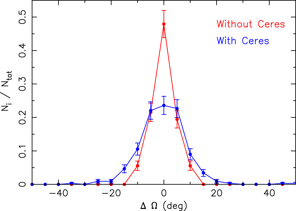
Figure 12 compares the distribution of Ω values obtained for $\tau =5.746$ Myr in our numerical simulations with and without Ceres (results for ϖ are similar). The distribution in the simulation with Ceres is clearly broader. We find that this is mainly a consequence of close encounters with Ceres. Of the 322 clones that converged within $\pm 10^\circ$ in a simulation without Ceres, roughly 80% converge within $\pm 10^\circ$ in a simulation with Ceres. The remaining 20% of the best clones do not converge so well. Of these, roughly 75% suffered close encounters to Ceres (within the Hill sphere or closer). A small fraction of clones suffered a very close Ceres encounter, and had ${\rm{\Delta }}{\rm{\Omega }}\simeq 30^\circ$ at $\tau =5.746$ Myr. On average, Ceres encounters add $\simeq 4^\circ$ to the dispersion of angles at the time of convergence. This limits the precision to which the convergence of angles can be determined, and therefore the accuracy with which the ${\rm{\Delta }}a$ values over the estimated age of the family can be computed: a difference of 4° corresponds to a difference of $7.2\times {10}^{-5}$ au in the ${\rm{\Delta }}a$ computed from the convergence of Ω and of $5.3\times {10}^{-5}$ au for that from ϖ. Including other massive asteroids in the simulation would slightly increase this threshold.

Zoom In Zoom Out Reset image size

The main results of this work can be summarized as follows.

• 1.  
  We revised the Karin family membership using the identification from Nesvorný et al. (2015) and initially including asteroids in the immediate neighborhood of the Karin cluster. The taxonomical and albedo interlopers were eliminated. We numerically integrated the orbits of all selected objects backward in time over 10 Myr. Using the convergence criteria described in the main text, we identified 576 asteroids that are very likely true members of the Karin cluster.
• 2.  
  Using the method of Nesvorný & Bottke (2004), we inferred the drift rates caused by the Yarkovsky effect. By minimizing the difference between two determinations of ${\rm{\Delta }}a$ from ${\rm{\Omega }}$ and $\varpi$, we found that the age of the Karin cluster is $\tau =5.746\pm 0.011$ Myr. This age determination is consistent with and improves on the previous estimate.
• 3.  
  Since the Yarkovsky drift rate depends on obliquity, we interpreted the observed distribution of the drift rates in terms of the obliquity distribution. For small, D = 1–2 km Karin cluster members, the distribution of obliquities is clearly bimodal. The best explanation for such a distribution is that the YORP effect acted to alter the distribution that was initially more uniform.
• 4.  
  We simulated the evolution of obliquities and spin rates with a simple Yarkovsky/YORP model. We found that the magnitude of the obliquity changes required to explain the bimodal distribution is consistent with the YORP effect and inferred age τ. The surface thermal conductivity is inferred to be 0.07–0.2 W m⁻¹ K⁻¹, corresponding to the thermal inertia of $\simeq 300\mbox{--}500$ J m⁻² K⁻¹ ${{\rm{s}}}^{-1/2}$). We find that the strength of the YORP effect is roughly $\simeq 0.7$ of the nominal strength obtained for a collection of random Gaussian spheroids. These results are consistent with a surface composed of rough, rocky regolith.
• 5.  
  We performed additional numerical simulations with the Yarkovsky drift and gravity of (1) Ceres. We found that the close encounters of Karin cluster members with Ceres act to increase the dispersion of angles and does not allow us, even in principle, to obtain a perfect convergence. On average, Ceres increases the dispersion of angles by $\sim 4^\circ$ at $\tau =5.746$ Myr.

Our work motivates new observational efforts. In particular, it would be interesting to verify the obliquity distribution inferred from our work. A decade ago, such a goal would have been a remote possibility, but recent advancements in asteroid shape and rotation state studies can lead to interesting results soon. For example, the obliquities of individual bodies can be obtained from the sparse photometry data of ground-based survey programs (e.g., Ďurech et al. 2016). Even more powerful results are expected from space missions such as Gaia (e.g., Mignard et al. 2007).

We thank the reviewer of this paper, Dr. Bojan Novaković, for comments and suggestions that improved the quality of this work. This paper was written while the first author was a visiting scientist at the Southwest Research Institute (SwRI) in Boulder, CO, USA. We would like to thank the São Paulo State Science Foundation (FAPESP) that supported this work via the grant 14/24071-7. D.N.'s work on this project was supported by NASA's Solar System Workings program, while D.V. was supported by the Czech Grant Agency (grant GA13-01308S). This publication makes use of data products from the Wide-field Infrared Survey Explorer (WISE) and from NEOWISE, which are a joint project of the University of California, Los Angeles, and the Jet Propulsion Laboratory/California Institute of Technology, funded by the National Aeronautics and Space Administration.

In Table 1, we report the list of 480 identified Karin cluster members. The table lists their absolute magnitude, proper elements $({a}_{P},{e}_{P},\mathrm{sin}{i}_{P})$, frequencies g and s, Lyapunov exponents (Lyapunov exponents with values near to $1.5\times {10}^{-6}\;{\mathrm{yr}}^{-1}$ correspond to objects for which the integration time was not long enough to obtain a convergence), estimated mean obliquity ε, and estimated mean Yarkovsky drift speed. Note to observers: the obliquity values listed in Table 1 are historical mean obliquities and may not exactly coincide with the current values. Figure 13 shows the correspondence between the historical obliquity values given in Table 1 and our estimate of the present obliquities.

Table 1.  Karin Cluster Members: Absolute Magnitudes, Proper Elements and Frequencies, Lyapunov Exponents, and Estimated mean Obliquities and Yarkovsky Drift Speed

Number	H	aP	eP	$\mathrm{sin}{i}_{P}$	gP	sP	LCE		Drift Speed
		(au)			($^{\prime\prime}$ yr−1)	($^{\prime\prime}$ yr−1)	(10−6 yr−1)	(deg)	$({10}^{-5}$ au Myr${}^{-1})$
832	11.18	2.86440	0.04390	0.03687	70.639	−65.235	1.49
10783	13.41	2.86480	0.04411	0.03683	70.676	−65.270	1.49	113	−0.84
11728	13.48	2.86555	0.04443	0.03676	70.746	−65.334	1.56	180	−3.10
13765	14.41	2.86967	0.04585	0.03688	71.112	−65.667	1.15	180	−5.33
13807	13.68	2.86885	0.04527	0.03682	71.037	−65.590	1.92	162	−2.54
15649	14.70	2.86418	0.04393	0.03650	70.632	−65.226	1.47	180	−4.50
16706	14.43	2.86200	0.04330	0.03676	70.435	−65.051	1.49	180	−4.86
20089	14.76	2.86170	0.04312	0.03696	70.402	−65.022	1.46	139	−3.10

Only a portion of this table is shown here to demonstrate its form and content. A machine-readable version of the full table is available.

Download table as:  DataTypeset image

Zoom In Zoom Out Reset image size