


ABSTRACT
We describe a new system and method for collecting coordinated occultation observations of trans-Neptunian objects (TNOs). Occultations by objects in the outer solar system are more difficult to predict due to their large distance and limited span of the astrometric data used to determine their orbits and positions. This project brings together the research and educational community into a unique citizen-science partnership to overcome the difficulties of observing these distant objects. The goal of the project is to get sizes and shapes for TNOs with diameters larger than 100 km. As a result of the system design it will also serve as a probe for binary systems with spatial separations as small as contact systems. Traditional occultation efforts strive to get a prediction sufficiently good to place mobile ground stations in the shadow track. Our system takes a new approach of setting up a large number of fixed observing stations and letting the shadows come to the network. The nominal spacing of the stations is 50 km so that we ensure two chords at our limiting size. The spread of the network is roughly 2000 km along a roughly north–south line in the western United States. The network contains 56 stations that are committed to the project and we get additional ad hoc support from International Occultation Timing Association members. At our minimum size, two stations will record an event while the other stations will be probing the inner regions for secondary events. Larger objects will get more chords and will allow determination of shape profiles. The stations are almost exclusively sited and associated with schools, usually at the 9–12 grade level. We present a full description of the system we have developed for the continued exploration of the Kuiper Belt.
Export citation and abstract BibTeX RIS
1. INTRODUCTION
Occultations of stars by solar system objects have long provided important data about sizes and shapes of asteroids and atmospheric structure. One of the first to recognize the power of this technique as applied to atmospheres was Fabry (1929). In this early work Fabry recognizes and describes many of the phenomena present during an observation of an occultation such as diffraction by a solid body edge and refraction by an atmosphere. At the time he was writing a purely theoretical description since the phenomena required high-speed observations that were essentially impossible in that era. In the nearly 100 years since, we have a formidable suite of tools that have been used to observe all of these aspects of occultations and more.
The biggest challenge to occultation-based studies remains the relative scarcity of suitable events. In general, a given object is rarely seen to occult a star. For example, it was not long after the discovery of Pluto that the search was on for occultation opportunities (e.g., Halliday 1963). The first unequivocal and well observed occultation of a star by Pluto was not until 1988 (cf. Elliot et al. 1989). The 58 year wait for the first occultation was due to the paucity of stars along Pluto's path as well as imprecise knowledge of the position of Pluto. In fact, prior to the discovery of Charon in 1978, an occultation was essentially impossible to predict due to the offset of the bodies from their mutual barycenter. That first occultation showed the presence of a substantial atmosphere that has since led to specific instrument designs for the New Horizons mission to Pluto (Stern et al. 2008; Tyler et al. 2008).
The first successful asteroid occultations began to be observed with some regularity in the 1970s (cf. Millis & Elliot 1979). For asteroids, there many bodies to choose from if you do not care which object does the occulting. Even so, the rate of successful measurements was a few per year from then until the late 1990s. In these early days it took a considerable effort to obtain a suitably good prediction of an occultation shadow path with enough warning to deploy ground stations to the right area. This epoch of occultation science was limited to professional astronomers using photoelectric photometers (e.g., Wasserman et al. 1977).
The quality of predictions increased dramatically with the release of a new high-quality star catalogs, eg., Hipparcos and Tycho, and their antecedent catalogs, USNO A/B and UCAC1-4 (Monet et al. 1998, 2003; Zacharias et al. 2004). These catalogs were sufficiently accurate that additional astrometric observations were no longer necessary and the known orbit of the asteroid and catalog position was sufficient to predict the shadow track. At this time, the amateur astronomy community began to seize these opportunities, and the number of asteroid occultations has increased to ∼100 per year. Along with this increase in observation rate, the amateurs have pioneered methods of observation using low-cost equipment that is capable of precise occultation timings (Timerson et al. 2009, 2013).
The discovery of the vast numbers of objects in the outer solar led to an obvious desire to use occultations to probe these objects. Their greater distance and relatively poorly known orbits make their occultation shadow paths at least as difficult to predict as main-belt asteroids were back in the 1970s. To date, almost all of the occultations by outer solar system objects have involved the brightest and largest of these objects. A bright object can easily be observed by modest sized telescopes to permit good orbit knowledge. A large object means the shadow is bigger, and it is easier to locate a telescope within the shadow.
The investigation into this region continues by the determination of physical characteristics of smaller, more numerous objects. The size distribution of the Kuiper Belt provides an important clue that constrains models of the formation of the solar system. Accurate size distributions rely on the ability to convert from apparent magnitude to diameter. So far, we know very little about the distribution of albedo or its variation with size. Additionally, there are a very high fraction of trans-Neptunian objects (TNOs) that are equal-mass binaries (cf. Noll et al. 2008). What we know about the prevalence of binaries comes largely from the Hubble Space Telescope but direct imaging always has a lower bound in resolution. Occultation observations are the perfect method to probe for binaries for smaller objects and for separations down to contact binaries.
Successful observations of occultations by 100 km TNOs using current techniques requires significant effort to obtain high-precision astrometry of every candidate object and star. Given that much of this work requires a 4 m class telescope or larger, this effort is generally practical only for a limited number of objects and then generally only the largest and brightest TNOs. Another method that will work with lower-quality and more infrequent astrometry is to deploy a large number of observing stations over an area much wider than the width of the shadow to be observed. In other words, the probability of success for an occultation observation is proportional to the number of deployed sites and scales inversely with the astrometric uncertainty. Increasing the number of stations by a factor of 10 will permit successful observations with predictions that are 10 times worse. These considerations drove the design of a new type of occultation system described here. With available technology, we designed a system that can probe objects down to D = 100 km in size and counter the relatively poor quality of the occultation event predictions. This system is now operational and the following sections describe system design, how it operates, and provides reference documentation for the observations yet to come. The companion paper Rossi et al. (2015) describes our first successful TNO campaign observation.
2. RECON DESIGN AND IMPLEMENTATION
The majority of the observations in this work were collected by team members of the Research and Education Collaborative Occultation Network (RECON). Additional observations were collected by members of the International Occultation Timing Association (IOTA). Though RECON was still under development at the time of the 2007 UK126 (Rossi et al. 2015), that observational campaign served as the first fully functional TNO occultation campaign for the project. In this section we describe the design and implementation of RECON.
2.1. Design
The normal methodology used for many decades in the occultation community was to strive for a ground-track prediction of the shadow path accurate enough to permit placing mobile stations in the shadow. This method imposes a requirement that the prediction of the relative position of the star and occulting body be known on a scale comparable to the size of the body. Meeting this requirement is not difficult for main-belt asteroids (MBAs). At 1 AU, the scale on the plane of the sky is 725 km arcsec−1. Using a notional size of D = 100 km (roughly HV = 9) at a geocentric distance of 1 AU, a differential astrometric precision of 0.14 arcsec will produce a prediction where the error is equal to the size of the object. The astrometric precision required gets linearly smaller with increasing geocentric distance. Thus, a TNO at 40 AU would require a precision of ∼4 mas to get the same predictive knowledge of the ground-track. Getting such an accurate prediction can be done but is at the level of the best ever done and requires a substantial effort on large telescopes for each prediction.
The core goal of RECON is to obtain occultation diameters on TNOs with D ≥ 100 km. This goal imposes two critical constraints. First, getting sizes of D = 100 km objects requires having a station spacing no greater than 50 km. Second, we must successfully put stations in the shadow track. Putting two mobile stations in the shadow requires requires predictions better than 4 mas predictions. This level of astrometric precision is not possible with current star catalogs without an unrealistic amount of time on a 4 m class telescope. Increasing the number of stations will cover a larger footprint and reduce the astrometric precision needed in proportion to the size of the footprint. Thus if you deploy enough stations to cover a region 10x bigger than the object, the astrometric precision required drops to 40 mas. The width of the network of stations thus sets the astrometric precision needed.
When an object is at opposition, its shadow track across the Earth is generally east–west. Therefore, to get good cross-track coverage it works best to spread out the stations along a north–south line. For mobile stations, telescopes should be spread out perpendicular to the track. For fixed stations a compromise is required and a north–south deployment strategy will, on average, be the optimum direction. For a mobile network there is no constraint on the placement of a station along the shadow track. As long as the object is up and the Sun is down, the data will be equally useful. In the case of a fixed set of stations, the gap between stations and the placement of the station relative to the shadow track will depend on the angle of the shadow track relative to the orientation of the station positions. Arranging the stations along a strict north–south line, with no east–west scatter will provide optimum coverage in all cases. The station spacing will depend only on the angle of the track to the station deployment line. As the amount of east–west scatter increases, sites will begin to duplicate each other and start leaving coverage gaps. This problem manifests if the amount of scatter approaches or exceeds the desired station spacing. Unfortunately, a strictly north–south deployment line for fixed stations is not practical but these considerations still guided the real-life plan for RECON.
Another strong consideration for a fixed network is weather. The network of sites is fiscally limited and is thus finite. To get the most data out of the infrastructure investment it is best to work with sites that have good weather. Our estimates of the number of TNO events per year indicates that we really do need mostly good weather to have a reasonable chance of getting useful data.
The final design consideration concerns the placement of the telescopes. Obviously, mobile stations would be the best for always being deployed cross-track with no coverage gaps and avoiding bad weather on the night of an event. The reality of this strategy is that for a D = 100 km object, only two sites out of the entire deployment will get to see the occultation. All of the other sites will get data but see nothing. For the notional design, this implies a probability of success for each station of 5%. The large spread of stations implies a very widespread, costly, and difficult deployment. Our concern is that even the most dedicated occultation observers will be unwilling to make a long-term commitment of effort for such a low personal chance for success, especially if the effort is considerable. Such high-effort, low-yield endeavors can be made to work in special circumstances but not for routine observations. Fixed-site observations have the advantage of minimizing the effort required and striking a balance with the expected yield. We considered building a network from those already doing occultations such as the members of IOTA. This option was dismissed since the IOTA participants are not numerous enough to be in all the locations we need for the project. To get the coverage required with IOTA resources would force us back to mobile deployments and is not tractable. Instead, the goal is to pick specific communities where a telescope can be permanently located. Thus, when it comes time for an event, the participants only have to take the telescope outside, set it up, and observe the event. We expect that by eliminating the effort to travel to a location and providing a telescope that is very easy to setup, we can minimize the effort and implement a viable network of telescopes.
The system design for occultation measurements of objects with D ≥ 100 km is thus driven by these four considerations: (1) large numbers of telescopes separated by 50 km, (2) establish stations along a north–south line, (3) locate span of telescopes where the weather is good across the network, and (4) place each telescope site in a community.
The weather constraint is best satisfied by a transect that runs along the western United States. Southeastern California and Arizona boast some of the best astronomical weather in the country. Northward from there, the best weather is seen in the rain shadow of coastal mountain ranges. We considered two viable options. Both options included sites along the Colorado River Valley which forms the border between Arizona and California. North of there we considered a track that ran from Kanab up through Salt Lake City and into Idaho. The other track follows the western side of Nevada up through Reno and then eventually through central Oregon and Washington. The eastern option was preferable due to a more regular spacing of cities and town along the path. The more westerly option was preferred, and chosen, for having significantly better weather prospects.
In almost all cases, there was no choice in picking communities. In this largely rural region of the western US, there are just enough locations to meet the needs of this project. However, some locations did require adjustments to ensure coverage. These implementation details will be covered in the next section. The biggest question remaining was where to physically locate the telescopes within the communities. Our focus, from the start, was to involve schools. Almost all of these communities have schools and provide a focal point for the region. We also recognized the potential for involving students and teachers in an authentic scientific investigation.
2.2. Implementation
In 2012 October we received funding from the National Science Foundation for a two-year pilot implementation of RECON. The first phase was to recruit the identified communities. During two separate trips, we met face-to-face with teachers or community members in Tulelake, Alturas, Bishop, Burney, Fall River, Greenville, Quincy, Portola and Susanville (in California), Reno, Carson City, Yerington, Hawthorne, and Tonopah (in Nevada). Everyone contacted was very interested and of these only one declined to take a lead role in the project. We were able to expand our search and recruit the nearby community Cedarville, CA, to fill that slot in the network.
Each community was encouraged to form a leadership team drawn from teachers, amateur astronomers, and community members with a strong emphasis on teachers. The goal of this group is to ensure a known contact for the project and to recruit students for participation in the project. The teams provide the year-to-year stability of the project while the students bring renewed enthusiasm each year. Having multiple team members protects against some people being unavailable for time-critical events as well as providing stability against attrition. We encourage teams of 4–6 people, and this is generally true except for the smallest communities. Once the teams were formed, we began sending equipment to the sites.
In 2013 April, we conducted a 4 day training session in Carson City, NV, at the Jack C. Davis Observatory. Each team sent two representatives to the training and brought their RECON equipment. During the training we provided presentations on the equipment and the scientific background of the project. Lectures were interspersed with daytime and nighttime activities to provide opportunities to practice with the telescopes and cameras. On the last night we conducted a simulated occultation observation to bring together all the project elements. At the completion of the workshop, all of the teams were ready to begin observing within the pilot network.
In 2014 September, we received full funding from NSF to implement and run the full network for five years. The original plan was to have a network of 40 telescopes. Through bulk purchasing arrangements we managed to get the per-station cost down below our original estimate. We also uncovered local resources in a few places to assist with procurement of the necessary equipment. We uncovered a few locations in the network where the spacing of communities led to gaps in coverage. In these locations we found extra communities along separate lines that, when combined, gives the desired coverage. Examples of this strategy can be seen in southern Oregon and south-western Nevada and California. Using these multiple tracks required recruiting and outfitting more stations and we were able to stretch our resources enough to cover the entire network. In north-central Washington we found more communities than we needed but they were all very enthusiastic and were able to contribute to the hardware purchase so we have a denser grid there than in other regions of the network. All together, a total of 56 telescope sites are now committed to the project.
The training for the extensions to the network were split into two regional efforts. The first was held in 2015 March in Kingman, Arizona for all of the sites south of the pilot network (Beatty to Yuma). The second was in 2015 April in Pasco, Washington for all of the sites north of the pilot network (Lakeview and Klamath Falls up to Oroville). We also brought one representative from each of the pilot stations to one of these training workshops. This provided an opportunity to either provide training to new team members of the pilot network or to bring seasoned members from the pilot to share their perspectives during the training and help pass on what they learned to new recruits. The full RECON network reached full operating status in 2015 April with the completion of the final training session.
The full list RECON sites is shown in Table 1 along with a map of the site locations in Figure 1. The first column, "Map ID," matches the number on the map. The name of the community is also given along with the nominal location of the community. The actual placement of the telescope during each event can and will change but not enough to affect the event coverage. In some cases, the site is a collaboration between multiple nearby communities and both sites are listed. The column, "Pop. (k)," gives the population of the community from the 2010 census to the nearest thousand except for the smallest communities where the population is given to the nearest hundred. The column, "System ID," is a permanently assigned code for the equipment in that community. The codes starting with "1" denote the original pilot project sites with the first batch of equipment (green circles in Figure 1). The codes starting with "2" denote the bulk of the new sites (blue circles). These systems are nearly identical to the pilot project. The camera is the same even though it was given a different product name. The IOTA-VTI units for these sites is an updated version from the pilot. The sites codes starting with "3" use the last batch of equipment (magenta circles). In this case, the basic camera design is the same but the sensor is a newer 2x higher efficiency detector. The IOTA-VTI units for these sites are an even more recent version. A few site codes are shown that start with "V," denoting a volunteer organization or individual (red circles). In this case, these teams provide their own equipment but work closely with the project and are full and equal partners in the project. A few of the new sites contributed a telescope but we provided the rest of the hardware. The telescopes for Oroville and Brewster were provided by the Central Washington University Gear Up Program. The telescope for Madras/Culver was provided by the Oregon State University SMILE Program.

Figure 1. Map of the RECON sites. The numbers on the map provide a cross-reference to the Map ID listed in Table 1. Green symbols indicate the pilot network sites. The blue symbols indicate the location of new sites with the standard sensitivity MallinCAM (same as the pilot network). The magenta symbols indicate the sites with the high-sensitivity camera (see Section 3.1). The red symbols indicate volunteer sites that contribute the use of their own facilities to the project (#37 was also part of the pilot network).
Download figure:
Standard image High-resolution imageTable 1. Site Summary
| Map ID | Community | Longitude | Latitude | Elev. (m) | Pop. (k) | System ID | Facilities |
|---|---|---|---|---|---|---|---|
| 1 | Oroville, WA | W119:26:21 | N48:56:04 | 286 | 2 | 3-01a | MS+HS |
| 2 | Tonasket, WA | W119:26:04 | N48:42:05 | 316 | 1 | 2-16 | HS |
| 3 | Okanogan, WA | W119:35:07 | N48:21:54 | 265 | 3 | 3-02 | HS |
| 4 | Brewster, WA | W119:47:15 | N48:05:38 | 242 | 2 | 2-17a | HS |
| 5 | Manson/Chelan, WA | W120:09:24 | N47:53:05 | 350 | 4 | 3-03 | MS+HS |
| 6 | Entiat, WA | W120:13:38 | N47:39:53 | 237 | 1 | 2-18 | MS+HS |
| 7 | Wenatchee, WA | W120:19:37 | N47:24:37 | 253 | 32 | 3-04 | HS |
| 8 | Ellensburg, WA | W120:32:52 | N46:59:47 | 470 | 18 | 2-19 | U/HS |
| 9 | Yakima, WA | W120:33:52 | N46:35:24 | 354 | 91 | 3-05 | HS |
| 10 | Toppenish/White Swan, WA | W120:23:41 | N46:22:26 | 240 | 9 | 2-20 | U/HS |
| 11 | Pasco, WA | W119:07:17 | N46:15:08 | 127 | 60 | V-02b | CC |
| 12 | Whitman College, WA | W118:19:48 | N46:04:18 | 287 | n/a | V-03b | U |
| 13 | Goldendale, WA | W120:49:18 | N45:49:14 | 499 | 3 | 3-06 | MS/SP |
| 14 | The Dalles, OR | W121:11:19 | N45:35:46 | 77 | 14 | 2-21 | HS/CC |
| 15 | Maupin, OR | W121:04:54 | N45:10:38 | 330 | 0.4 | 3-07 | MS+HS |
| 16 | Madras/Culver, OR | W121:07:25 | N44:37:49 | 689 | 6 | 2-22a | HS |
| 17 | Sisters, OR | W121:34:34 | N44:17:46 | 984 | 2 | 2-23a | HS/AC |
| 18 | Redmond, OR | W121:10:26 | N44:16:21 | 914 | 26 | 3-08 | HS |
| 19 | Bend, OR | W121:18:55 | N44:03:29 | 1105 | 77 | 2-24 | K12/HS |
| 20 | Oregon Observatory, OR | W121:26:49 | N43:53:05 | 1268 | 1 | V-04 | SC |
| 21 | LaPine/Gilchrist, OR | W121:30:25 | N43:40:47 | 1290 | 2 | 2-25 | MS/HS |
| 22 | North Lake, OR | W120:54:10 | N43:14:42 | 1345 | 1 | 2-26 | K12 |
| 23 | Paisley, OR | W120:32:34 | N42:41:36 | 1329 | 0.2 | 2-27 | K12 |
| 24 | Chiloquin, OR | W121:51:48 | N42:34:03 | 1277 | 0.7 | 2-28 | MS+HS |
| 25 | Klamath Falls, OR | W121:46:54 | N42:13:30 | 1252 | 21 | 2-29 | HS/CC/U |
| 26 | Lakeview, OR | W120:21:01 | N42:11:09 | 1450 | 2 | 2-30 | MS+HS |
| 27 | Tulelake, CA | W121:28:44 | N41:57:19 | 1232 | 1 | 1-01 | MS+HS |
| 28 | Cedarville, CA | W120:10:24 | N41:31:45 | 1420 | 0.5 | 1-02 | HS |
| 29 | Fall River/Burney, CA | W121:23:56 | N41:02:45 | 1012 | 4 | 1-03 | MS+HS |
| 30 | Susanville, CA | W120:39:19 | N40:24:55 | 1279 | 18 | 1-04a | HS |
| 31 | Greenville, CA | W120:57:04 | N40:08:23 | 1098 | 1 | 1-05 | MS+HS |
| 32 | Quincy, CA | W120:56:50 | N39:56:13 | 1050 | 2 | 1-06 | HS/CC |
| 33 | Portola, CA | W120:28:10 | N39:48:39 | 1492 | 2 | 1-07 | MS+HS |
| 34 | Reno, NV | W119:49:06 | N39:32:42 | 1387 | 225 | 1-08 | U/HS |
| 35 | Carson City, NV | W119:47:47 | N39:11:09 | 1446 | 55 | 1-09b | HS/CC |
| 36 | Yerington, NV | W119:09:39 | N38:59:28 | 1340 | 3 | 1-10 | HS |
| 37 | Gardnerville, NV | W119:44:59 | N38:56:29 | 1449 | 6 | V-01 | AA |
| 38 | Hawthorne, NV | W118:37:49 | N38:31:35 | 1321 | 3 | 1-11 | HS |
| 39 | Lee Vining, CA | W119:07:17 | N37:57:40 | 2060 | 0.2 | 2-01 | HS |
| 40 | Tonopah, NV | W117:12:51 | N38:03:30 | 1880 | 3 | 1-12 | HS |
| 41 | Bishop, CA | W118:23:42 | N37:21:49 | 1264 | 4 | 1-13 | HS |
| 42 | Lone Pine, CA | W118:03:40 | N36:36:08 | 1135 | 2 | 2-02 | HS |
| 43 | Beatty, NV | W116:45:29 | N36:54:04 | 999 | 1 | 2-03 | HS |
| 44 | Indian Springs, NV | W115:40:36 | N36:34:27 | 965 | 0.9 | 2-04 | K12/AC |
| 45 | Henderson, NV | W114:58:54 | N36:02:22 | 569 | 258 | 2-05 | HS/CC/AC |
| 46 | Searchlight/Boulder City, NV | W114:55:11 | N35:27:55 | 1079 | 0.5 | 2-06 | ES/HS/AC |
| 47 | San Luis Obispo, CA | W120:39:45 | N35:18:18 | 97 | 45 | 1-14 | U/HS |
| 48 | Kingman/Dolan Springs, AZ | W114:03:11 | N35:11:22 | 1021 | 28 | 2-07 | K12/MS/HS/AC |
| 49 | Laughlin/Bullhead City, NV | W114:34:23 | N35:10:04 | 163 | 47 | 2-08 | MS+HS |
| 50 | Mohave Valley, AZ | W114:34:00 | N34:53:42 | 144 | 14 | 2-09 | HS |
| 51 | Lake Havasu City, AZ | W114:19:04 | N34:29:39 | 259 | 53 | 2-10 | MS/HS/AC |
| 52 | Parker, AZ | W114:17:19 | N34:08:33 | 127 | 3 | 2-11 | HS |
| 53 | Idyllwild, CA | W116:42:42 | N33:44:03 | 1639 | 4 | 2-12a | SC |
| 54 | Blythe, CA | W114:35:18 | N33:37:04 | 81 | 21 | 2-13 | AC/HS/CC |
| 55 | Calipatria, CA | W115:31:28 | N33:07:30 | −56 | 8 | 2-14 | HS |
| 56 | Yuma, CA | W114:37:40 | N32:41:34 | 62 | 93 | 2-15 | HS/LIB/PR |
Notes.
aSites providing their own telescopes but we provided the rest of the equipment. bSites providing all of their own equipment. Positions are given on the WGS84 datum. See text for additional details.Download table as: ASCIITypeset image
Over time there will be changes in the involved team members and we also hope to attract additional self-funded volunteer stations, particularly in southern Arizona. We already have informal expressions of interest from people in the Tucson area and will specifically target the region from Phoenix down to Nogales for extra coverage to shore up the extreme southern end of the network. Discussions are also underway with astronomers from UNAM about an independent extension of RECON into Mexico tracking down the Baja peninsula. The facility codes in the last column indicate which type of facility or institution is involved in the primary community: AA—amateur astronomer, AC—astronomy club, CC—community college, ES—elementary school, HS—high school, K12—K-12 school, LIB—library, MS+HS—typically a combined 6–12 or 7–12 school, PR—parks and recreation, SC—science center, SP—state park, U—university.
The standard equipment provided is listed in Table 2. The telescope is a computer controlled alt-az mounted system that is very easy to assemble and align to the sky. Once aligned, the system can point to a desired target and generally place the star in the camera field of view (FOV). The choice of a 28 cm aperture size was dictated by cost, size and weight, and ease of setup. Larger sizes are much more difficult to setup and are significantly more expensive. A smaller telescope would have fewer candidate events. The video camera is specially designed to permit integrating on the target up to 2.1 s while maintaining a standard NTSC video signal. An in-depth discussion of the camera and data recording can be found in the next section. All of the equipment, except for the laptop, is powered from an external 12 V battery pack.
Table 2. Equipment List
| Item | Description | Cost |
|---|---|---|
| Celestron CPC110 | Schmidt–Cassegrain f/10 telescope with a 28 cm aperture. Telescope is computer controlled and has a GPS for position and time during setup and is operated in alt-az mode. | $3000 |
| Telrad finder | Unit-power finder for rough acquisition of alignment stars. | $45 |
| Focus mask | A hard-plastic Bahtinov-type focusing mask used for accurate telescope focusing. | $20 |
| Dew shield | Passive plastic dew shield that attaches to the front of the telescope to partially shield the front corrector from radiatively cooling to the night sky. | $40 |
| Storage box | Hard-plastic wheeled container. | $65 |
| MallinCAM RECON 428 or 828 | Special-purpose integrating video camera using a SONY HAD detector (1/3 inch). Provides NTSC video output but allows for setting the integration time in multiples of frames up to 64 (∼2 s). | $700 |
| MallinCAM MFR-5 | 3x focal reducer with extra 5 mm spacer provides an f/3.3 beam. Its outer diameter is 1 1/4 inches and fits in a standard eyepiece holder. | $250 |
| IOTA-VTI | Video timing box. This box includes a GPS receiver that then superimposes the current time on each video field as it passes from the camera to the computer. | $250 |
| Laptop Computer | Small netbook format computer running Windows 7. Used for event planning with OccultWatcher and video data collection with VirtualDub. | $300 |
| USB to Video adapter | Adapter for connecting the video output from the camera to the computer. | $45 |
| Miscellaneous | Various short power and video cables and splitters as well as spare fuses. | $100 |
| Portable Power Pack | Rechargable battery pack. This provides power to the telescope, camera, and video timer. | $50 |
| Storage Box | Water and dust tight plastic storage box to hold everything other than the telescope. | $13 |
| $4878 |
Download table as: ASCIITypeset image
3. CAMERA AND DATA SYSTEM
This section provides detailed information about the performance and operation of the camera and associated data system. Information is also included on how to apply the timing data to return accurately timed light curve observations.
3.1. Camera
The camera chosen for this project is specially made by MallinCAM. This product was an early mainstay of the MallinCAM product line until suitable products were developed for color video imaging. The detectors for color imaging have very complicated pixel structures and lower overall sensitivity. Our occultation observations require the highest absolute sensitivity and a gray-scale system is much preferred. The cameras are assumed to be unfiltered with a quantum efficiency curve of a typical CCD detector. The old design was pulled out of retirement for this project and can be made to order as long as the detectors are available.
The MallinCAM was chosen on the basis of performance test results that compared the sensitivity of cameras popular within the IOTA community. We tested the Watec 120N+, Watec 910HX, MallinCAM Jr, and Super Circuits PC165DNR which are all capable of doing frame-integration. Additionally, we tested the Watec 902H3 and Super Circuits PC104 non-integrating cameras. The non-integrating cameras all had better data quality when compared in a non-integrating mode. However, without frame integration the limiting magnitude is not faint enough for this project.
The MallinCAM Jr and PC165DNR were especially attractive for their significantly lower price. Their sensitivity was actually quite good but the cosmetic quality of the data was noticeable worse. There were strong odd–even row and line noise. Some component of this noise is due to a fixed pattern but light curve data taken with similar integration times had a markedly lower signal-to-noise ratio (S/N) than the chosen camera.
The Watec cameras had essentially identical performance as the MallinCAM under dark-sky conditions. The Watec 120N+ has long been a mainstay of the occultation community despite being the most expensive camera of this type. Unfortunately, this model has been discontinued and has been replaced by the Watec HX. This newer camera is somewhat cheaper and was supposed to have better sensitivity and image cosmetics. Unfortunately, the control interface for the new camera is much more complicated and requires an add-on controller that was doubtful to survive heavy use.
A digital detector normally has a much higher dynamic range and resolution than what can be transmitted in an NTSC video signal. After integrating frames, the dynamic range is even higher. All such digital camera systems must map the intensity from the image onto the range of valid signal levels in the output video. All of the systems have the option of using automatic gain controls but this mode cannot be used when a photometrically accurate signal is desired. In all tests, we set the cameras to manual control and maximum gain.
There is one fundamental difference between the Watec and MallinCAM systems that gave the MallinCAM a strong advantage. For long integration settings, the Watec will nearly saturate with a bright background such as will be seen near a brightly illuminated moon. This difference is how the cameras handle the black level in the image. The Watec cameras have a set black level that depends on the gain and integration time. With no illumination, this level is just enough above zero that you can see the readout and background noise level. In the presence of illumination the background level will vary depending on how bright the illumination is. Therefore, when the moon is down and there is no nearby light pollution, the Watec will show a low black level. If the moon is up or if there are nearby lights making the sky brighter, the background level will increase and will increase in direct proportion to the frame integration length. As this happens, the available dynamic range on the video signal is reduced, limiting the photometric precision possible on the target source. The MallinCAM appears to have a circuit that automatically adjusts the black level. The adjustment is slow, significantly longer than a frame integration length. However, the background level will change from frame to frame, even if the frame is a replication from a long integration. One might assume that adjacent video frames within an integration would be identical and would show up in a simple difference of the DN values between frames. This situation appears to hold for the Watec camera but not for MallinCAM data. Another test is to look at the standard deviation of the difference between adjacent frames. With this metric, a drifting mean is ignored and the frame boundaries are revealed as a change when crossing a frame boundary. Note that this test is also sensitive to the proper frame/field alignment. Unfortunately, this test is not effective on 100% of the data. Sometimes it works perfectly well and other times it completely fails. We will return to this issue in Section 3.2 where we discuss time calibration of occultation data.
Another key aspect of the camera system is matching it to the focal plane of the telescope. The MallinCAM is sold with a barrel adapter that screws into the front face of the camera and fits into a standard 1 25 eyepiece adapter. If used in this manner, the FOV is too small and the light from stars is too spread out, diminishing the overall sensitivity and making target acquisition extremely challenging. With the addition of a focal reducer, the field is increased and the spot size of a star is reduced. The common recommendation from the IOTA community was to use a 3x focal reducer. We tested two such units, one made by Meade Instruments and the other by MallinCAM. If properly mounted, both provided equivalent results however getting a proper mount for the Meade unit required a custom made part. The MallinCAM MFR5 is a very compact assembly that can be reconfigured for differing amounts of focal reduction. The assembly also directly screws into the camera, ensuring the proper back focal position, and is also compatible with standard 125 eyepiece holders. We use the MFR5 with both optical elements with one 5 mm spacer in between the optics and the camera. This combination gives a ∼3x focal reduction and provides good image quality across the field. Adding more spacers further increases the focal reduction but at the expense of ever increasing amounts of aberration in the off-axis images. The final FOV of the camera and focal reducer is 16.9 by 12.7 arcmin with an image scale of 1.585 arcsec pixel−1. This field is reasonably well matched to the pointing accuracy of the CPC 1100. The pointing error from a slew is about the same size as the field. Many times the target star will be in the field after a slew but if not, it will be just outside the initial field. It is standard practice for our project to use a star diagonal to prevent interference of the camera and its cables with the telescope fork when pointed near the zenith. The orientation of the camera is standardized to put the direction to the zenith up in the image.
After most of the equipment was purchased, a new higher-sensitivity version of our MallinCAM became available. Eight of these were purchased and are deployed in the northern tier of the network, starting with Oroville and alternating with the regular camera southward through Redmond. The system IDs in Table 1 starting with "3-" are those with the higher-sensitivity cameras. This newer camera has roughly twice the sensitivity of the older model. We note that the newer camera coupled with a cheaper 20 cm telescope has nearly the same sensitivity as our original camera with a 30 cm telescope.
The MallinCAM with the focal reducer achieves SNR ∼ 10 for a visual magnitude 16 star in 2.1 s. Figure 2 shows a rough estimate of senseup (frame integration) setting as a function of target star brightness along with the SNR to expect under clear conditions. For any given senseup setting, the per-integration SNR ranges from a high of ∼20 at the bright limit to ∼5 at the low limit. Not included in this figure is the influence on spectral type of the star. A red star will lead to higher S/N than a blue star with the same visual magnitude. One of the most difficult tasks with this system on event night is picking the senseup setting to use. Under photometric conditions one can use the pre-determined value from a more careful analysis. If the conditions are variable then one must resort to guesses for a correct value. The risk and the common tendency is to choose a senseup value that is too large. When the integration time is too long the star will be saturated and the event timing is degraded. Unfortunately, tools for video capture do not have any features that permit evaluating the data in real time so that saturation can be avoided.
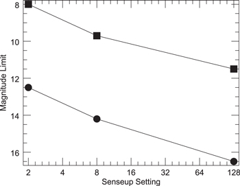
Figure 2. Useful magnitude range vs. senseup. The top curve (with squares) is the saturation limit. The bottom curve (with circles) is the faint limit. All values taken with the standard sensitivity MallinCAM with a CPC1100 telescope (28 cm aperture).
Download figure:
Standard image High-resolution image3.2. Timing
The timing unit we use is the IOTA-VTI, a device that was designed and manufactured by members of IOTA. It is powered using the same 12 V DC power supply as used for the telescope and camera. The timer is built around a GPS receiver that maintains time and position information. The signal from the camera is connected to the input, passed through the timer, and the output is connected to the storage device. In the normal mode of operation the timer will superimpose the current time on each field of the video stream. Also included is a field counter that increments by one for each field since the unit was powered on. This counter provides backup information in case the time were to jump during a recording. The time is given to the nearest 100 microseconds. The time display is placed at the bottom of the image leaving most of the image unobstructed for the actual star field. Alternatively, the VTI can superimpose the observing location on the image. This information is recorded by flipping a switch and is done for a short time once per event, usually before the event during setup.
Another complication for deriving accurate timing is in dealing with the frame integration time, referred to as "sense-up," in the video camera settings. If sense-up is turned off, the video signal is the normal interlaced image data. One consequence of this is you are only recording half of the signal at any given time (odd rows or event rows) with a subsequent loss of sensitivity. When sense-up is enabled, a new mode of imaging is used where the entire detector (odd and even rows) is exposed at the same time for the full duration of the integration. After exposing, the image is read out to memory and then is copied to the video data stream with the interlaced pattern. The image is copied to video for sense-up/2 frames. Thus at a sense-up setting of 2, the image is the result of a full 1/30 s integration and will have twice the integrated signal of a non-sense-up mode. The sense-up mode will also lessen noise caused by image motion that is near the field sampling rate.
There are some significant yet somewhat subtle features of working with video data that are worth a detailed explanation. Figure 3 provides a graphical summary of how the data goes from the imaging device to a file on the computer. To simplify this discussion, we review a few terms related to NTSC video. First, the video signal is a serial data interface where each pixel is transmitted in turn in the form of a DC voltage level during the appropriate time window relative to the sync signal. It takes roughly 1/30 of a second to transmit one image. The actual number is 29.97 (60/1.001/2) frames per second but it is common to round this to an integer 30 frames per second for purposes of discussion. This unit of data is called a frame and is a complete view of the field (orange boxes in Figure 3). However, the format of the signal is interlaced meaning that the even and odd rows of pixels in a frame are transmitted as two separate and alternating groups (green boxes). Each set of either odd or even rows (but not both) is referred to as a field. It takes roughly 1/60 of a second to transmit one field. Thus a frame is made up of two fields.
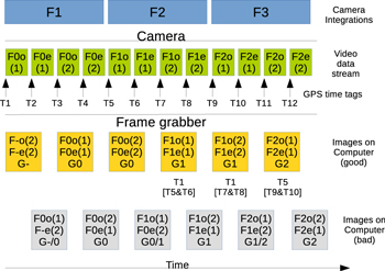
Figure 3. Simple timing diagram of image handling during data collection.
Download figure:
Standard image High-resolution imagePresented in Figure 3 is a timeline of how information flows during the collection of video data. This figure is drawn for a senseup value of 4x. This means the integration time of a frame is 4 fields long as shown in the figure (roughly 1/15 s). As soon as an image is read out it is then transmitted onto the video signal. Here you see F1 coming out as F1o (odd rows of frame 1), followed by F1e (even rows of frame 1). One more copy of F1 is transmitted to fill the time until the current integration F2 complete. The numbers in parentheses indicate which copy of a image is present. At the same time the images are coming out, the signal is passing through the IOTA-VTI. The black arrows mark the time at which the transmission of a field begins and thus each field carries a unique and advancing timetag. As you can see, data from the first image carries four different time tags (T5–T8).
As this point, the images are processed by the frame grabber and computer. Two fields are grabbed and combined to regenerate the original image. The orange boxes indicate a normal acquisition of fields and the resulting images. Inside the box is listed the name (field and copy number) of the fields that were combined. The label G1 indicates the frame-grabbed copy of image F1. As denoted immediately below, the time that F1/G1 started to be acquired is at T1. The image data contains the IOTA-VTI timestamp from T5 and T6. Thus, to get the mid-time of F1, you take the earliest time tag seen on copy 1 of G1 and subtract half of the integration time. In the case of senseup = 4x, the integration time is 1/15 s, so you subtract 1/30 s from T5 to get the mid-time. This sequence of images is what you get when the frame grabbing is done correctly.
The synchronization of the frame grabber to the video signal does not deterministically do this. It is possible for the frame grabber to be off by one field in its assembly of the data. This is shown schematically by the gray boxes. In this case, you alternate between a reasonable copy of the original image interspersed with image where the odd and even components are taken from different images. This stream of images looks nearly the same but if there is an occultation, the edge will appear to have an intermediate point mid-way between the low and high signal level on both sides of the event. Rephasing the fields into frames will eliminate this problem. With care, the need for rephasing can be deduced for 2x and 4x senseup settings. With longer senseup values it becomes very obvious.
This timing diagram implies that you know the starting time for an image. In reality, this is another bit of information that must be deduced form the data. In the case of a successful observation of a sharp occultation edge, these edges are easy to identify. Figure 4 shows some example edges with synthetic data. Panel (B) shows the case illustrated in Figure 3 for sense-up = 4x. The blue squares show the data that results from the frame integrations. The photometry from the transitional point on the light curve establishes the time of the edge of the event, limited only by the S/N in the images. The yellow points show flux from each grabbed image tagged by the time from the GPS timer. These data represent the raw light curve that can be extracted from the video. The raw light curve is adjusted by dropping the second point and subtracting half of the integration time from the time tags on the images. The gray points show the raw light curve in the case where the video interlacing is incorrectly phased. In this case you see three transitional points instead of one.

Figure 4. Synthetic light curve examples. The three panels show example simulated video light curve data. Panel (A) shows the case for SENSEUP = 2X and (B) and (C) show 4X and 8X, respectively. The color coding of the curves matches the diagram in Figure 3. The solid black curve shows the perfect resolution light curve from an occultation assuming no diffraction effects and no angular size to the star. The blue line with tick marks shows the boundaries for the frame integrations. See text for further details.
Download figure:
Standard image High-resolution image
The case shown in panel (C) is for sense-up = 8x and is even more obvious. The correct raw light curve has four identical points for the four copies of the integration. The incorrect phasing gives two extra intermediate points and only 3 identical points.
The case shown in panel (A) using senseup = 2X is the most challenging setting to get precise timing for this system. In this case of perfect SNR, it is still easy to see the swapped case because there are two transitional points. In reality, low SNR or finite stellar angular diameters can create transitional edges that look very similar to this example. In the case of the RECON project, we expect to work with fainter and thus more distant stars that will tend to have very small angular diameters. Upon inspection of the images, swapped fields can sometimes reveal a striped star image while the other case will show a normal image at half the signal as long as the star image is not undersampled. With sufficient effort and SNR, it is possible to figure out the correct phasing. However, a 2X senseup setting is the least likely option we will use as most of our target stars will be much fainter and require more integration.
To summarize, once the field order and frame boundaries are correctly identified, read the time code from the first field of an integration. Assuming negligible time for readout and data handling to get the image to the video data stream, this time code is the start time of the next image that will be seen on the video. Thus, if you have the start time values as read from the video data, the mid-time of each frame is given by

where tm is the mid-time of the integration in seconds, t0 is the time imprinted on the first field of the integration converted to seconds, S is the sense-up setting (ranges from 2 to 128 for the MallinCAM).
3.3. Data Collection
The video signal is then collected with frame grabbing software on the laptop. We use the program VirtualDub with the Lagarith lossless encoder to save the video data to disk. The data rate for this setup is about 200 Mb minute−1. A common problem encountered while collecting data is an inaccurate depiction of the incoming video on the screen. The data often look darker leading to a tendency to choose significantly longer integration times than are desired.
Typical main-belt asteroid occultations have small errors on the predicted times and a few minutes of data is usually sufficient. During the pilot phase of the project we found this to generate very manageable data files and all data were transmitted electronically via the internet. The timing uncertainties are significantly longer for TNOs and a normal data collection window is 20–30 minutes. Single files covering the entire window are quite large (4–6 Gb) and difficult to transmit.
Before we settled on the laptop and video grabbing software, we used low-cost digital video recorders (DVRs). There were some very attractive features of these units: they can automatically break video into user configurable durations (eg., 5 minutes per file), are very simple to operate, have a built-in monitor, cost $45 per unit, have independent battery power, and generate small video data files. This last feature, small file sizes, turned out to be a fatal flaw. To get the small size, the unit has a built-in codec that uses aggressive lossy compression. The DVRs also shifted the video signal to a lower black level. The input signal from the MallinCAM has a well chosen black level within the video range but the DVR shift moved the background to a hard-zero level. Pushing the background below zero means the photometry is significantly compromised since you no longer have any information on where the zero-signal level is in the system. Also, without the sky background, you cannot discover the frame integration boundaries or even figure out what the frame integration time was in those cases where insufficient documentation exists for the data. These units are not completely useless since you can still determine ingress and egress to no worse than the length of the integration time. For the test events in the pilot project we tended to work with brighter stars so the timing errors were not too large. In the case of our Patroclus observations (Buie et al. 2015), a senseup of 2X was used meaning the times could be no worse than 1/30 s. The Patroclus event was the last where we used the DVR after which we switched to the laptop and frame grabber setup.
We tested a number of options for grabbing video data with VirtualDub. The options fall in three broad categories: uncompressed video, lossless video compression, and lossy video compression. The lossy compression results in very small and quite manageable file sizes but unfortunately the data quality suffer significant degradation. In particular, most of the noise in the background is eliminated, similar to the problem with the mini-DVR. Uncompressed video clearly preserves all of the input data but suffers from occasional dropped frames on our computers. Our guess is that the sustained I/O rate is just a little too high for periodic latencies inherent in the Windows operating system used by our systems. By using a lossless video encoder, the data rate to be written to disk is reduced enough that dropouts during a write to disk are eliminated. The resulting files are about a factor of two smaller than uncompressed video. We tested both the Lagarith and UtVideo codecs and got very similar performance from both. The Lagarith codec gave marginally smaller files and we decided to standardize on this option. On our systems, we can record indefinitely with no dropped frames with the Lagrith codec. The recording limit is set only by the size of the hard disk.
The final stage of the data collection process is posting results. The teams are encouraged but not required to process their own data. However, all teams are required to send their data to SwRI for archiving as well as the final data reduction process. During the phase where we used the mini-DVR's a simple internet browser-based system was sufficient for uploading those small files. In the final production system the files were too big for this process. Presently we use an rsync-based data transfer method that is resilient against slow and interrupted network connections. It still takes a long time (many days) to collect all the data from a TNO event but the process eventually works. The data collection system is also setup to permit any team member to download any data from another team. This facilitates classroom exercises that teachers might wish to conduct using actual RECON data sets.
4. PREDICTION SYSTEM
There are many resources available from which to learn about interesting occultation events. Within the RECON project, we have a strong guideline that campaign events must be announced at least one month before the event to give our teams time to coordinate their schedules and prepare for the observation attempt.
4.1. IOTA-NA
The North American chapter of the International Occultation Timing Association (IOTA-NA) maintain lists of asteroid occultation predictions. These are provided through web pages, email notifications, and most importantly as a prediction feed that is used by OccultWatcher (hereafter referred to as OW). This software system, developed by IOTA member Hristo Pavlov from Australia, collects information from any suitable formatted set of predictions and filters them according to the observer's preference such as limiting magnitude and prediction uncertainty. OW also provides a means for observers to sign up for events. A registered user can then see all of the sites that have signed up for an event and see where their location falls relative to the predicted ground track. This serves to show where gaps in coverage exist so that interested observers can easily spread out to provide more complete coverage without unnecessary duplication.
Within RECON, we use OW to keep track of our sites by asking them to sign up for each campaign event. At present, not all of the events we pursue can be found in OW but we are working to improve this situation. Everyone in RECON as well as the greater IOTA community can then see the aggregate coverage for the event. Also, we use this as a tool to ensure that each site is, in fact, engaged for each campaign without the need for extensive effort by direct email or telephone contact. When OW cannot be used we use a simple online form that our teams fill out.
The IOTA feeds, including the ones specially constructed for North America, are usually updated once a month. This lead time is more than sufficient for the normal flow of IOTA activities where decisions tend to be made very close to the time of the event. This amount of lead time has been problematic for RECON and more than a few good opportunities have been passed over due to lack of sufficient warning. However, the focus of IOTA thus far has really been on main-belt asteroid occultations, though Jupiter Trojans are also on their watch list. RECON has pursued main-belt occultations but mostly as a training exercise. The focus for our project, especially with the full network, is on TNO events.
4.2. Rio Group
One active group in the field of TNO occultations is a collaborative effort between Assafin and Braga-Ribas in Brazil and Sicardy in France with considerable observational effort employed from Brazilian facilities. These efforts are aimed at high-precision predictions on the brightest TNOs, basically limited by the data possible from a 2 m class telescope. This group has been very successful in obtaining occultation sizes using the "classical" chase-the-shadow approach. Most of the largest TNOs now have occultation sizes, for example Eris: D = 2326 km (Sicardy et al. 2011), Makemake: 1430 × 1502 km (Ortiz et al. 2012), Quaoar: 1039 × 1138 (Braga-Ribas et al. 2013). Most of their successful observations have been obtained from South America but they do not restrict their prediction efforts based on geographic location of the shadow tracks. More recently, this group has created its own OW feed that covers the TNO prediction work they conduct. One of the most recent examples of such a prediction is described in the companion paper (Rossi et al. 2015) which is the first successful RECON TNO event. Within the RECON project, we monitor and consider all events from the "Rio feed" for potential campaigns. This feed usually provides ample warning on events but so far is limited in only working on the brighter TNOs. This sample is usually significantly larger than the 100 km size we wish to measure.
4.3. SwRI/Lowell System
Within RECON, we must also do our own prediction work to ensure sufficient opportunities of objects at the minimum targetable size of D = 100 km. For the purposes of choosing potential targets we consider anything with  to be a candidate for observation. This limit includes a significant fraction of the objects in the cold-classical TNO population—a group that is under-represented in TNO occultations thus far. As of 2015 February there were 1694 designated TNOs (including Centaurs). Of these, 1458 have
  . Some of those objects are effectively lost at this point. The 910 objects with uncertainties less than 4 arcmin are the sample of objects to search for occultation events. Table 3 shows a summary of the known TNOs and the effective sample size that is under consideration. Shown is the rough breakdown of objects according to dynamical class using the Deep Ecliptic Survey system (Elliot et al. 2005; Gulbis et al. 2010; Adams et al. 2014). Here the tabulation breaks down the sample into three bins by astrometric uncertainty. The numbers in parentheses indicate the percent of the objects in that bin are fainter than
  . This tabulation clearly shows the under-representation of the smaller and fainter objects in the pool needed for successful occultations.
Table 3. Occultation Event Candidates
| Type | Total |

|

|

|
|---|---|---|---|---|
| Centaur | 69(20%) | 13(0%) | 40(15%) | 16(50%) |
| Resonant | 250(50%) | 11(18%) | 163(45%) | 76(66%) |
| Classical | 355(72%) | 16(38%) | 227(67%) | 112(87%) |
| Scattered | 232(45%) | 18(17%) | 147(42%) | 67(60%) |
| Total | 910(55%) | 58(19%) | 578(51%) | 274(72%) |
Download table as: ASCIITypeset image
We have constructed a prediction system with an associated observing protocol for continued astrometric observations with 4 m class telescopes ensuring a good sample down to D = 100 km. One goal is to eliminate the large error objects to make them searchable for events. Prior to the start of the pilot project, this was the largest category. Our efforts in the past two years, together with L. Wasserman at Lowell Observatory, have moved most into the middle category. For any object with σ ≤ 2, we search for candidate appulses that pass with 5''. Those objects with no appulses are dropped from the astrometric observational program. Those with appulses are targeted for additional astrometry to get the positional uncertainties to σ ≤ 0.2 and these are then considered for observational campaigns.
The prediction system is an augmentation of the orbit classification system from the Deep Ecliptic Survey (Millis et al. 2002). This system runs once a day to look for TNOs with new or updated astrometry. The orbits are refit for any object with updates and then they are newly classified. A notification is distributed for any object whose classification changed. We have added a new layer to this system that identifies objects that have improved orbits and then updates the prediction for their occultations. The calculations performed depend on the observational history of the object and the current and future uncertainties in position.
A coarse search is run on low-error objects (σ ≤ 2 arcsec at 2 years) to find all appulses less than 5 arcsec with V > 17 stars in the next two years. This coarse list is updated on the first of each month by adding the time not yet searched in the next two years as long as the 2 year uncertainty remains below 2 arcsec.
Occultation event predictions are then generated for all appulses where the TNO positional uncertainty is less than 4000 km. Events observable from Earth are then saved while noting those relevant to RECON. In the case where an object already has identified events and there is an updated orbit, the prediction is updated.
A key element of this appulse list processing and selection of campaign events is the estimated uncertainty in the ground-track location. We have the ephemeris uncertainty for all TNOs that can be computed for the time of event. We actually compute a error ellipse for the position, but for the class of objects that we can predict occultations, the ellipse has collapsed down to a line. This line is known as the line of variations (LOV). The direction of the LOV is computed by taking the nominal position and then recomputing a new position with a very small change to the mean anomaly of the object's orbit. For a well constrained orbit, this characterization of the positional error is a very good approximation. The LOV can be, but is not usually, parallel to the object's motion on the plane of the sky, though they are roughly in the same direction most of the time. The LOV error can thus be broken into two components, parallel to the target motion and perpendicular to the target motion. The parallel component will manifest as an error in the time of the occultation. The perpendicular component is an error in the location of the ground track. We use this procedure to compute these two components of error for every prediction. At the end we add a uniform component of error to both that is ascribed to the uncertainty in the position of the star. This latter error is certainly not zero but in most cases is very difficult to determine with any accuracy. Note that this treatment does not make any attempt to quantify the inevitable systematic errors in both the TNO orbits and the star catalog positions. As long as these errors do not exceed 0.1 arcsec, it is possible to predict events that are within reach of RECON. For the purposes of our prediction system we add 50 mas of error for the star to each event unless there are actual measurement errors. Our estimate is that we need a minimum success rate of about 30% per event, not counting weather, for RECON to be successful. This rate sets the minimum success probability for an event we will choose for a full campaign.
Predictions for all events are automatically maintained on a publicly accessible web site3 and email notifications are sent for any notable changes in the prediction list. Note that the system is built to automatically process any astrometry that is published by the Minor Planet Center, augmented by any astrometry we have or have been provided to us that is not yet published by the MPC. Routine observations from the community are thus automatically included and affect predictions.
5. SAMPLE OBSERVATIONS
Observations by the pilot RECON sites began in 2013 May. Table 4 shows a summary of the events attempted and their results to date. There are three types of attempts described here. The first is an official campaign where the entire network is expected to be on the field taking data. Moving forward, this will only happen for TNO events. Regional campaigns are a sub-category where a specific set of sites is expected to observe an event. This would be used for an event with a sufficiently small ground-track uncertainty that not all sites are needed. This sub-category is not expected to be very common. Another category is an optional activity where we identify an interesting main-belt or perhaps Jupiter Trojan object that can be done with some or all of RECON (usually a subset of the sites). In this case, team members are merely encouraged to make a best effort to observe the event with no requirement that they do so. This type of event is particularly useful as training and practice in between the official campaigns. The third category contain events that are identified by RECON team members on their own. These events are usually main-belt asteroids. In this case, it is then left up to the RECON teams to promote regional campaigns with nearby sites. It is recognized, though, that official campaigns have priority over all other categories of event.
Table 4. Pilot Network Campaign Summary
| UT of Event | Object | Star mag | Size (km) | Comment |
|---|---|---|---|---|
| 2013 Feb 11 06:48 | (451) Patientia | 11.2 | 234 | pre-training activity |
| 2013 Apr 18 05:40 | (211) Isolda | 12.2 | 154 | optional |
| 2013 May 04 08:22 | Pluto | 14.4 | 2320 | first full campaign |
| 2013 May 06 11:10 | (225) Henrietta | 12.5 | 149 | optional |
| 2013 Jul 03 09:22 | (83982) Crantor | 14.6 | 60 | optional |
| 2013 Jul 11 07:30 | (1910) Mikhailov | 11.1 | 37 | regional campaign |
| 2013 Jul 16 05:15 | (25) Phocaea | 11.2 | 83 | regional campaign |
| 2013 Jul 30 06:45 | (387) Aquitania | 12.3 | 123.4x89.3 | regional campaign |
| 2013 Aug 03 04:48 | (2258) Viipuri | 9.5 | 27 | self-organized campaign |
| 2013 Aug 24 06:13 | (489) Comacina | 11.5 | 168.5 × 111.0 | full campaign |
| 2013 Sep 01 03:49 | (7) Iris | 11.3 | 200 | self-organized campaign |
| 2013 Oct 06 09:53 | (227) Philosphia | 11.1 | 87 | self-organized campaign |
| 2013 Oct 17 11:49 | (339) Dorothea | 11.4 | 46 | self-organized campaign |
| 2013 Oct 21 06:46 | (617) Patroclus | 9.6 | 124.6 × 98.2,117.2 × 93.0 | optional |
| 2013 Nov 09 06:07 | (176) Iduna | 11.9 | 142.5 × 113.1 | full campaign |
| 2013 Nov 17 05:26 | (607) Jenny | 11.3 | 63 | self-organized campaign |
| 2014 Jan 15 04:10 | (16368) Citta di Alba | 10.3 | 17 | self-organized campaign |
| 2014 Feb 16 14:05 | (976) Benjamina | 12.4 | 85 | optional |
| 2014 Mar 03 09:10 | 2001 XR254 | 14.0 | 230 | optional |
| 2014 Apr 06 03:26 | (56) Melete | 13.2 | 134 | optional |
| 2014 Apr 26 04:43 | (1332) Marconia | 12.2 | 50 | full campaign |
| 2014 Jun 13 05:50 | (471) Papagena | 13.6 | 157 | self-organized campaign |
| 2014 Jul 15 06:33 | (1177) Gonnessia | 13.0 | 93 | full campaign |
| 2014 Jul 16 06:38 | (240) Vanadis | 13.5 | 107 | optional |
| 2014 Jul 27 05:30 | (429) Lotis | 13.1 | 73 | full campaign |
| 2014 Sep 14 11:58 | (404) Arsinoe | 12.3 | 117 | self-organized campaign |
| 2014 Sep 18 06:41 | (82) Alkmene | 7.7 | 64 | self-organized campaign |
| 2014 Oct 12 12:23 | (598) Octavia | 10.4 | 78 | self-organized campaign |
| 2014 Oct 21 04:22 | (225) Henrietta | 11.3 | 113.5 | optional |
| 2014 Nov 15 10:43 | (229762) 2007 UK126 | 15.8 | 600 | full campaign |
| 2014 Nov 16 02:44 | (230) Athamantis | 10.8 | 108 | self-organized campaign |
| 2015 Jan 20 03:54 | (702) Alauda | 11.3 | 219 | self-organized campaign |
Download table as: ASCIITypeset image
Most of the campaigns shown in Table 4 involve relatively bright stars. These events are typical of main-belt asteroids. In the case of main-belt asteroids, the asteroids themselves are often bright enough to be easily detected with our systems. As the brightness difference decreases between target and star, it becomes more difficult to make an accurate measurement since the target only adds to the background noise. The target brightness is never an issue for TNOs and Centaurs allowing us to work with much fainter stars.
The first full campaign we attempted was the 2013 May 04 Pluto occultation. The early predictions still had the ground track near our stations but later refinements showed the track running over South America. This event was unlikely to yield a positive observations but we felt it would be a good first practice event. This event was also very challenging for being a pre-dawn event with Pluto rising low in the southeast. This is among the most difficult events we have thus far attempted. The success rate for this first event was not 100% nor was it expected to be so. Our teams gained valuable experience and insight that left them better prepared for events yet to come.
The strategy behind regional campaigns is to provide an experience where the outcome is likely to be a positive occultation for as many participating sites as possible. Since most of our TNO campaigns will result in misses for most sites, it is important to provide opportunities to gain experience with positive results. Main-belt asteroids, in collaboration with IOTA can provide useful training exercises where an actual event is seen. These opportunities will usually engage a small fraction of the network per event. Another strategy for these main-belt events comes with observations of objects nearer to quadrature. In these cases the shadow tracks can have a large north–south component, reducing the projected spacing between sites and yielding a higher spatial resolution across the objects. The events with (387) Aquitania, (489) Comacina, and (176) Iduna are particularly good examples of this strategy which led to the determination of an elliptical limb profile.
The (617) Patroclus event would have been an excellent campaign had the full network been ready at that time. As it was, most of the sites were north of the ground-track and only a special mobile effort put RECON gear in the shadow. A complete analysis and discussion of the Patroclus event can be found in Buie et al. (2015). This event is an excellent proto-type for the TNO binaries we hope to measure over the course of the project.
Many of the events in 2014 were identified and used to maintain proficiency and engagement of the pilot network. As the full network was developed our attentions turned toward TNO events. Fortuitously, a TNO event was identified by the Rio group that was expected to be near the RECON pilot sites. The last full campaign listed in Table 4 is much more like the events RECON is designed to observe, except for the larger target size. The prediction was better than we expect for normal RECON events and was practical for the pilot network sites. A more complete description of those observations are in the companion paper Rossi et al. (2015).
6. CONCLUSIONS
RECON is a new project for probing TNOs and is now fully functional. The description of the project provides our initial baseline of procedures and practices to help document future work. However, this is a living project and system and will likely evolve and grow as we better learn to use this novel scientific and observational resource.
Thanks to Gordon Hudson for the Meade focal reducer test mount. Thanks to Chris Cotter, John Zannini, and Don McCarthy for very early discussions about the project design. At CalPoly, thanks are due to Belyn Grant for her enthusiastic support, especially during the first wave of recruiting, Andrew Parker and Jeralyn Gibbs during the development of the full network, Kaylene Wakeman and Rosa Jones for logistical and other support, and Steve Pompea for early discussions about the project. We also thank Columbia Basin College Robert & Elisabeth Moore Observatory, Sisters Astronomy Club, The Bateson Observatory, Western Nevada College Jack C. Davis Observatory, and Guided Discoveries Astrocamp for their support of this project. Finally, this project would not be possible without all of the support from our community teams: teachers, students, and community members. This work is was funded by NSF grants 1212159 and 1413287.