


ABSTRACT
The solar magnetic activity is governed by a complex dynamo mechanism and exhibits a nonlinear dissipation behavior in nature. The chaotic and fractal properties of solar time series are of great importance to understanding the solar dynamo actions, especially with regard to the nonlinear dynamo theories. In the present work, several nonlinear analysis approaches are proposed to investigate the nonlinear dynamical behavior of the polar faculae and sunspot activity for the time interval from 1951 August to 1998 December. The following prominent results are found: (1) both the high- and the low-latitude solar activity are governed by a three-dimensional chaotic attractor, and the chaotic behavior of polar faculae is the most complex, followed by that of the sunspot areas, and then the sunspot numbers; (2) both the high- and low-latitude solar activity exhibit a high degree of persistent behavior, and their fractal nature is due to such long-range correlation; (3) the solar magnetic activity cycle is predictable in nature, but the high-accuracy prediction should only be done for short- to mid-term due to its intrinsically dynamical complexity. With the help of the Babcock–Leighton dynamo model, we suggest that the nonlinear coupling of the polar magnetic fields with strong active-region fields exhibits a complex manner, causing the statistical similarities and differences between the polar faculae and the sunspot-related indicators.
Export citation and abstract BibTeX RIS
1. INTRODUCTION
Solar magnetic activity, most apparent by the coming and going of dark sunspots and bright faculae in the photosphere and the eruptive phenomena (e.g., flares, prominences, filaments, and coronal mass ejections) in the upper solar atmosphere, exhibits a cyclic regeneration of the appearance of the Sun that occurs with a dominant periodicity of about 11 years (Sheeley 2008; Yan et al. 2009; Feng et al. 2013; Charbonneau 2014; Clette et al. 2014). The long-term variation of the solar cycle can be described by many solar activity indicators, such as sunspot number, sunspot areas, polar faculae, Hα flare index, total and spectral solar irradiance, Mg ii index, Ca ii K plage index, filament counts, 10.7 cm radio flux, coronal index, coronal holes, coronal mass ejections, and so on (Frohlich 2012; Solanki et al. 2013; Tlatov et al. 2014; Lefevre & Clette 2014; Yeo et al. 2014). Most of them are highly correlated with each other as they are intrinsically inter-linked through solar magnetism and its dominant 11-year Schwabe cycle. Apart from many common features, they also show obvious differences, as well as on short- and long-term trends. This is because the compared indicators are related in various ways to different aspects of physical processes operating in the Sun. Hathaway (2010), Usoskin (2013), and Ermolli et al. (2014) reviewed the physical and synthetic indicators that are utilized to describe the solar magnetic activity cycle, moving from the ones referring to direct observations of the inner solar atmosphere (photosphere and chromosphere), to those deriving from measurements of the transition region and solar corona. The availability of solar time series has a large potential impact not only on solar physics research, but also on space weather and studies of the Earth's climate. Therefore, the statistical properties (e.g., quasi-periodic variation, hemispheric coupling, phase relationship) of different solar time series have become a topic of great interest and research in recent years.
The solar activity cycle is modulated by several quasi-periodic cycles showing period-doubling characteristics and aperiodic grant minima with a characteristic timescale exceeding several tens of periods (Barnhart & Eichinger 2011). Schwabe (1844) described an irregular behavior with fluctuations in the cycle duration as well as in the individual shape and maximum intensity. Feynman & Gabriel (1990) suggested that the solar dynamo exhibits chaotic behavior and is very close to the bifurcation between period-doubling behavior and chaos, because the Maunder-type minima have reoccurred irregularly for millennia and the 88-year Gleissberg cycle of the solar magnetic activity disappeared from the Maunder minimum. Based on the reconstructed phase spaces of the solar magnetic activity cycle, Rozelot (2007) interpreted the disappearance of this prolonged periodicity in terms of phase changes of the solar magnetic activity cycle. The author also depicted the phase catastrophe during the Dalton minimum (1790–1820), likely leading to a lost numbered cycle. Usoskin & Mursula (2003) pointed out that the solar activity cycle is not perfectly regular: the cycle length and amplitude, the ascending and descending durations, and the shape of the maxima vary from cycle to cycle. The global aspects of the solar activity cycle are well explained by the solar dynamo theories, but it is not clear whether the solar dynamo behaves like a chaotic or a stochastic system, that is, whether the irregularities of the solar activity cycle can be explained as deterministic dynamics or stochastic processes (Letellier et al. 2006). There are several reasons intrinsic to solar physics why the irregular behavior of the solar activity is of interest. First, it has implications for the solar dynamo theories, which, according to the present ideas, should characterize the physical processes that control the observed manifestations of the solar magnetic activity (Hanslmeier et al. 2013). Second, it is important both for procedures predicting the solar activity cycle and for reconstructing solar time series on different temporal scales (Hanslmeier & Brajsa 2010). Finally, the spatio-temporal irregularity, or the dynamical complexity, is an intrinsic property of the solar magnetic activity (Consolini et al. 2009). Understanding the intrinsic properties of different solar time series helps to better characterize the different aspects of magnetic processes taking place on the Sun, but presently it is either unknown or not comprehensively known. Although the chaotic and fractal properties of solar magnetic activity have been studied and observed extensively in the past few years using a variety of solar activity indicators, including sunspot number, sunspot areas, Hα flare activity, facular numbers, 10.7 cm radio flux, and cosmogenic radionuclide 10Be and 14C data (Watari 1996; Lepreti et al. 2000; Hanslmeier & Brajsa 2010; Hanslmeier et al. 2013; Ghosh et al. 2014; Zhou et al. 2014), sometimes the analysis results derived from different approaches are completely opposite. For an unambiguous detection of a low-dimensional chaotic behavior of solar magnetic activity, we need to wait for longer and more reliable time series to be available (Carbonell et al. 1994; Panchev & Tsekov 2007). Mininni et al. (2002, 2004) suggested that the spatio-temporal irregularity observed in the solar magnetic activity is not a plain manifestation of a low-dimensional chaos, due to the interaction of two superposed antisymmetric modes with a stochastic background. Consolini et al. (2009) found that the emergence of dynamical complexity excludes the hypothesis that the solar magnetic activity is caused by a low-dimensional chaos or purely stochastic process. They proposed that the observations of a low-dimensional chaos in the sunspot time series could be the consequence of the use of coarse-grained descriptors, which are unable to convey all of the information contained in spatio-temporal diagrams. However, Letellier et al. (2006) showed that the 22-year solar magnetic cycle, as reconstructed by sunspot time series, is in agreement with a low-dimensional chaotic behavior. In detail, they show that the phase-space diagram of the sunspot time series resembles a Rossler dynamical system. They concluded that using the appropriate cover of the sunspot cycle could help to unfold the dynamics and provide a better observability of the dynamics. Similar analysis results were found by Li & Li (2007), who investigated the group sunspot number during the time interval from 1825 January to 1995 December, and by Zhou et al. (2014), who studied the chaotic and fractal properties of the sunspot numbers and sunspot areas from 1874 November to 2012 December, and by Zou et al. (2014), who measured the correlation dimension and K2 entropy of full-disc, low-latitude, and high-latitude solar filament numbers from 1919 March to 1989 December. Moreover, Aurell et al. (1997) studied the predictability problem in dynamical systems with many degrees of freedom and a wide spectrum of temporal scales. They found that the intermittency correlations do not change the scaling law of predictability, and they also discussed the relation between the finite-size Lyapunov exponent and information entropy.
The magnetic fields of the Sun's poles are thought to be the direct manifestation of the global poloidal fields. They are the seed fields of the global dynamo model and produce the toroidal fields that result in the formation of sunspot and active regions (Jin & Wang 2011; Jiang et al. 2013). The study of the polar magnetic field is important for understanding the mechanism of the solar activity cycle and the origin of the solar wind acceleration, and the latter's extension to the interplanetary magnetic field. Information from the polar magnetic fields is also used to predict the strength of the next solar cycle (Schatten et al. 1978; Choudhuri et al. 2007). Polar faculae are bright, small-scale structures visible in white-light observations and in chromospheric lines. They populate higher heliographic latitude  above 60° or 70°. The number of polar faculae is considered to be an ideal proxy for the polar magnetic fields (Sheeley 2008). Similar to the sunspot-related indicators (sunspot numbers or sunspot areas), the polar faculae take part in the solar activity cycle and follow a periodicity of 11-year Schwabe cycle (Erofeev & Erofeeva 2000; Tlatov 2009), with a phase shift by 5–6 years, with respect to the sunspot-related indicators (Makarov & Makarova 1996; Deng et al. 2013). The faculae become visible after the reversal of the polar magnetic fields around the sunspot maximum, and their numbers reach a maximum at the sunspot minimum (Makarov et al. 2003). The relationship between the polar faculae and sunspot activity, i.e., the nonlinear coupling of the polar magnetic fields with the active-region fields described in Babcock–Leighton models, makes the faculae as valuable for studying the poloidal part of the solar activity cycle as the sunspots are for studying the toroidal aspect of the solar activity cycle (Munoz-Jaramillo et al. 2012). To better understand the statistical similarities and distinctions between the polar faculae and sunspot activity, it is necessary to compare their temporal properties from different points of view. Studies on the interconnection of the polar faculae with sunspot activity are of great importance to understanding the solar dynamo actions, especially with regard to the nonlinear dynamo models. This motivates us to compare the chaotic and fractal properties of the polar faculae with sunspot activity by means of nonlinear analysis techniques such as the phase portrait reconstruction, the rescaled range (R/S) analysis, and the largest Lyapunov exponent.
Since the Sun exhibits nonlinear dissipative behavior, traditional linear analysis techniques are inappropriate for determining the dynamical complexity of the solar time series. To investigate the irregular behavior of the polar faculae and sunspot activity, both the qualitative and quantitative analysis approaches are utilized to investigate their chaotic and fractal properties. The remainder of the present work is organized as follows. Section 2 provides a brief description of the time series used in this paper. Subsequently, the analysis approaches and the obtained results are revealed in Section 3. Finally, we summarize our findings and draw our conclusions in Section 4.
2. OBSERVATIONAL DATA
The three different time series analyzed in this work are as follows.
(1). Polar faculae were recorded on the sunspot sketches made with the Zeiss 20 cm refractor at Mitaka of the National Astronomical Observatory of Japan (NAOJ). The monthly counts of polar faculae can be publicly downloaded from NAOJ's website5 (Irie et al. 1993; Hagino et al. 2004; Hanaoka 2013). The time series covers the time interval from 1951 August to 1998 December at three latitudinal bands on both hemispheres: 50°–60°, 60°–70°, and 70°–90°. Sakurai (1998) stressed that the faculae observed at the latitudinal band 50°–60° are comprised of two components: one belonging to the low-latitude activity cycle and the other to the high-latitude activity cycle. Therefore, we only take into account the facular counts at the latitudinal bands 60°–70° and 70°–90°. We believe that by combining the facular counts at these two latitudinal bands and on both hemispheres the reliability and accuracy of the time series may increase (Deng et al. 2014).
(2). Sunspots are the most commonly known of the many manifestations of solar magnetic fields, which structure the Sun's atmosphere and make it variable (Solanki et al. 2006). The sunspot number is used mainly as proxies of solar activity and as tracers of the dynamo processes responsible for the build-up of large-scale magnetic fields into the solar atmosphere (Charbonneau 2014). Sunspot numbers indicate a weighted estimate of individual sunspots and sunspot groups derived from visual inspection of the solar photosphere in white-light integrated radiation. As the number of sunspots increases, the total sunspot area naturally increases and free magnetic energy within sunspots and their magnetic complexity usually grow as well; consequently, both small-scale and large-scale eruptive events increase (Xiang et al. 2014; Xiang & Kong 2015). The production, preservation, and dissemination of sunspot numbers are provided by the World Data Center-Sunspot Index and Long-term Solar Observations (WDC-SILSO) at the Royal Observatory of Belgium (Berghmans et al. 2002). Monthly reports of the sunspot numbers and the online catalog can be downloaded from their website.6 The time series of sunspot numbers is from 1874 May to 2015 August and is routinely updated every month. We extract the time interval from 1951 August to 1998 December, the common period of the polar faculae.
(3). The sunspot areas are given in units of millionths of a solar hemisphere. The monthly counts of the sunspot areas can be taken from the Royal Greenwich Observatory (RGO) archive and the National Aeronautics and Space Administration (NASA) website.7 The RGO compiled sunspot observations from a small network of observations to produce a time series of daily observations beginning in 1874 May. Sunspot areas are considered to have more physical significance than sunspot numbers or group sunspot numbers (Preminger & Walton 2007; Ermolli et al. 2014) due to the linear relation between sunspot areas and the total magnetic flux of a sunspot. Additionally, the time series of sunspot areas have additional information on the position (latitude and longitude) of the observed features, with respect to the time series of the sunspot numbers (Hathaway 2010). Moreover, the measurements of sunspot areas are the main input data to models of total magnetic flux and solar irradiance variations (Preminger & Walton 2006; Krivova et al. 2010).
To remove the short-term fluctuations and to reveal the long-term trends, the above three time series are smoothed with a 13-point running average method. In Figure 1, we plot the monthly counts of polar faculae (left panel), sunspot numbers (middle panel), and sunspot areas (right panel), respectively.
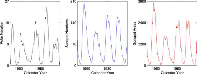
Figure 1. Monthly counts of polar faculae (left panel), sunspot numbers (middle panel), and sunspot areas (right panel) during the time interval from 1951 August to 1998 December.
Download figure:
Standard image High-resolution image3. METHODS AND RESULTS
The nonlinear effects in the solar activity cycle have been extensively studied in theoretical models and reviewed by several authors (Panchev & Tsekov 2007; Spiegel 2009; Arlt & Weiss 2014). Besides, nonlinear analysis techniques have been applied to predict the next solar activity cycle (Ghosh et al. 2014). In principle, it is still an open question whether the solar activity cycle can be explained as a chaotic or a stochastic system (Hanslmeier & Brajsa 2010; Hanslmeier et al. 2013). In the present paper, we first apply qualitative analysis methods to determine whether the solar time series is chaotic or random, and then quantitative analysis methods are utilized to calculate their complexity indicators, including the Hurst exponent, the fractal dimension, the predictability indicator, and the largest Lyapunov exponent.
3.1. Qualitative Analysis Methods
3.1.1. Phase Space Reconstruction
To investigate the nonlinear behavior underlying a scalar time series  the first step is to reconstruct an m-dimensional phase space (Packard et al. 1980). Two different coordinate sets can be used, i.e., the delay and the derivative coordinates (Takens et al. 1981). According to Takens' theory, the reconstructed phase space y, constructed mathematically from the time series x, can be defined as:
where τ is the time delay and m is the embedding dimension. It is necessary to calculate the appropriate values of these two parameters before reconstructing the phase space. As pointed out by Takens et al. (1981) and Sauer et al. (1991), if the sequence x consists of the scalar measurements of the state of a dynamical system, then the time delay provides a one-to-one image of the original time series x. It should be emphasized that this technique deals with the infinite, noise-free trajectories of a dynamical system, but is not guaranteed to hold for the finite series of the measured data (Schreiber 1999). Therefore, we have to assume that the results of the analysis in this paper are valid for the limited, and not the noise-free, time series.
In this paper, we apply the mutual information method (Fraser & Swinney 1986) to calculate the time delay of each time series. To estimate the embedding dimension, we use an algorithm written by Cao (1997) based on the false nearest neighbor method.
3.1.2. Mutual Information Method
The mutual information metod, which was first proposed by Fraser & Swinney (1986), is used to estimate the time delay of a chaotic time series. According to the information theory, the mutual information of two variables X and Y can be defined as

where fXY (x, y) is the joint probability density function of X and Y , and fX (x), fY (y) are the probability density functions of X and Y, respectively. Assuming a partition of the domain of X and Y, the double integral becomes a sum over the cells (Kantz & Schreiber 1997). For a scalar time series  sampled at equal distant interval τs, the mutual information between x(i) and x(i + τs) is defined as a function of the time delay τ. It can be described as
where P[x(i)] and P[x(i + τs] are the probability density functions of the time series x(i) and x(i + τs), respectively. An appropriate choice of the time delay for the embedding is one such that the mutual information is at a minimum. That is to say, if the mutual information exhibits a marked minimum at a certain value of τ, then it is a good candidate for a reasonable time delay. More information can be found in the papers of Fraser & Swinney (1986), Kantz & Schreiber (1997), and Hegger et al. (1999).
Figure 2 displays the results of the mutual information method as a function of time delay. The graphs are given for polar faculae (left panel), sunspot numbers (middle panel), and sunspot areas (right panel). From this figure, one can see that the profiles of the mutual information method for three time series slightly differ from each other. The reasonable time delays are found to be 31 months for polar faculae, 29 months for sunspot number, and 31 months for sunspot areas.

Figure 2. Variations of the mutual information method as a function of the time delay for polar faculae (left panel), sunspot numbers (middle panel), and sunspot areas (right panel).
Download figure:
Standard image High-resolution image3.1.3. False Nearest Neighbor Method
As the original attractor of the considered system is unknown, one should attempt to reconstruct an attractor that preserves the invariant characteristics of the original attractor. Based on Taken's theorem, an m-dimensional phase space can completely capture the nonlinear behavior of a given time series under the condition m ≥ d, where d is the embedding dimension of the original attractor (Karakasidis & Charakopoulos 2009). For an infinite and noise-free time series, the embedding dimension m can be determined by Takens' theorem. As proved by Takens' theorem, it is sufficiently to reconstruct the attractor under the condition m ≥ 2d + 1. However, it should be emphasized that the condition m ≥ 2d + 1 is sufficient but not necessary, because an original attractor may sometimes be reconstructed triumphantly with an embedding dimension as low as d + 1. If the embedding dimension m is too low compared to the dimension d of the attractor, the attractor displays self intersections, spatially nearby points on the attractor are either real neighbors due to the system's dynamics or false neighbors due to the self intersections. In a higher dimension, where the self intersections are resolved, the false neighbors are revealed as they become more remote. One tries to find a threshold value for m where no false neighbors are identified as one moves to increased dimensions. Here, we used the false nearest neighbor method, which was proposed by Kennel et al. (1992), to determine the minimal sufficient embedding dimension m. Using Takens' theorem one can estimate the dimension of a possible attractor.
The fundamental principle of the false nearest neighbor method is to increase the dimension of the phase space up to the point where there are no longer any self intersections of the trajectory. Based on Takens' theorem, Cao (1997) defined a parameter E1(d)—the relative change in the average distance between the two contiguous points—when the dimension is increased from d to d + 1. If the relative changes in the average distance saturate around 1, then the embedding dimension is equal to the minimal dimension. Moreover, another parameter E2(d) was proposed to discriminate the deterministic system from the stochastic process. For a random process, the future values are independent of the past values, so the values of E2(d) are equal to one for any dimensions. For a chaotic system, the values of E2(d) are not constants for all dimensions and they are related to the embedding dimension of the considered system. It should be pointed out that different time delays may bring out different embedding dimensions, especially for the time series from continuous temporal–spatial systems (Cao et al. 1998). An appropriate choice of the time delay will decrease the embedding dimension, which is necessary for phase-space reconstruction, as suggested by Letellier et al. (2006). That is to say, choosing a range of the time delays for which the embedding dimension does not change constitutes a suitable parameter that actual properties of the dynamical behavior are identified (Rhodes & Morari 1997). For more details of the false nearest neighbor method, the interested reader is referred to Kennel et al. (1992), Cao (1997), and Cao et al. (1998).
Figure 3 displays the variations of the parameters E1(d) and E2(d) as a function of the dimensions for polar faculae (left panel), sunspot numbers (middle panel), and sunspot areas (right panel). From this figure one can see that the profiles of E2(d) for three time series are not straight lines, providing strong evidence that the three solar time series analyzed in this paper exhibit a chaotic behavior. Moreover, their embedding dimensions are all equal to three, implying that both the high- and low-latitude solar activity are governed by a low-dimensional chaotic attractor, i.e., a three-dimensional phase space should be sufficient to properly unfold the underlying nonlinear behavior of the Sun. Previous studies have shown that the attractor dimension (D2) of the low-latitude solar activity (e.g., sunspot numbers and sunspot areas) is around 3, such as  (Mundt et al. 1991), D2 = 2.4 ± 0.2 (Kremliovsky 1994) and D2≈3 (Letellier et al. 2006). Therefore, the embedding dimension of sunspot activity is consistent with that reported by previous authors. Furthermore, our result provides convincing evidence that the chaotic behavior of the high-latitude solar activity should also be low-dimensional.
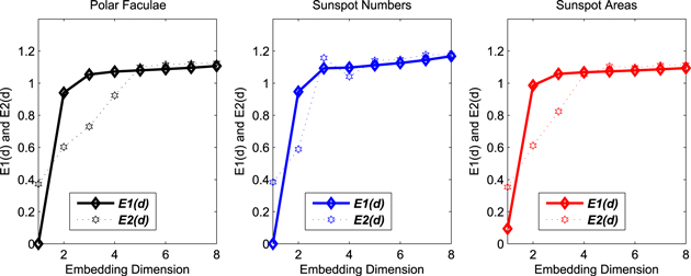
Figure 3. Variations of the parameters E1(d) and E2(d) as a function of the dimensions for polar faculae (left panel), sunspot numbers (middle panel), and sunspot areas (right panel).
Download figure:
Standard image High-resolution imageAfter estimating the time delay and embedding dimension of each time series, in Figure 4 we plot the reconstructed phase spaces for polar faculae (left panel), sunspot numbers (middle panel), and sunspot areas (right panel). From this figure, one can see that the phase portraits for the three time series are not like "balls of wool" (i.e., totally unfolded), and there seem to be some intrinsic structures underlying the considered systems. Here, we must keep in mind that the smoothing procedure can remove part of the original dynamics (the ideal situation is to remove only the stochastic component), but it cannot inject the nonlinear dynamics into the time series (Letellier et al. 2006). The stranger attractors characterized by the infinite self-similarity structures are clearly revealed, which are the one of the typical properties of the chaotic system. By comparing their complexities shown in the reconstructed phase spaces, we find that the chaotic dynamics of polar faculae are the most complicated, followed by that of the sunspot areas, and then the sunspot numbers. This is the first clue to support the hypothesis that the chaotic dynamics of high-latitude solar activity is more complicated than low-latitude solar activity.

Figure 4. Reconstructed phase spaces with the estimated parameters (time delay and embedding dimension) for polar faculae (left panel), sunspot numbers (middle panel), and sunspot areas (right panel).
Download figure:
Standard image High-resolution image3.2. Quantitative Analysis Methods
3.2.1. R/S Analysis
Historically, the first approach to quantify the long-range persistence of a time series was proposed by Hurst (1951), who spent his life studying the hydrology of the Nile River, in particular, the record of floods and droughts. To better reveal the long-term correlation of his empirical data, he introduced R/S analysis. This approach is based on the random-walk theory. Its predominant concept was developed at a time (1) when computers were in their early stages, so calculations had to be done manually, and (2) before fractional noises or motions were introduced. Currently, the use of R/S analysis is still popular and often applied. In this section we apply R/S analysis to investigate the long-range correlation and the fractal property of the above three time series.
R/S analysis is a simple but a strong nonparametric method for fast fractal analysis (Das et al. 2009). It is performed on the discrete time series X(i) of dimension N by calculating three factors: first the mean  second, R, which is the range of commutative difference of X(t, s) at discrete time t over a time span s, and third, the standard deviation S(i), estimated from the observed values of X(t, s), where

and
The range of cumulative difference of the time series is given by

where Y(i) is defined as

Hurst found that the ratio (R/S) is well described for the long-term time series of natural phenomena by the following experimental relationship (Hurst 1951):

where s and H are the time span and the Hurst exponent, respectively. The slope of the plot of R/S versus the time span s on log–log plot gives rise to H. The value of H indicates whether a time series is random or successive increments in time series are not independent. For H equals to 0.5, the time series represents a random walk, or is uncorrelated, and each observation is fully independent of all prior observations. The value of 0 < H < 0.5 indicates that it exhibits an anti-persistence behavior, i.e., its trend will likely reverse in the future. The value of H lying between 0.5 and 1 implies persistent time series characterized by long-range effects. The successive increments are positively correlated with the preceding observations (Kilic & Golbasi 2011).
To characterize the type of the self-affinity and the fractal property of solar time series, the Hurst exponents of the polar faculae, the sunspot numbers, and the sunspot areas are calculated by R/S analysis. Figure 5 shows the log–log plots of R/S as a function of the time span s, which estimates the values of the Hurst exponent H = 0.7692 ± 0.0525 for polar faculae, H = 0.7400 ± 0.0684 for sunspot numbers, and H = 0.7729 ± 0.0672 for sunspot areas, respectively. Since the H values of the three time series are larger than 0.5, this indicates that both the high- and low-latitude solar activity show persistence on large scales. The Hurst exponents of the three time series analyzed in this paper are agreement with those reported by previous authors, whose studies focused on the sunspot numbers (H = 0.86 ± 0.05; Mandelbrot & Wallis 1969; H = 0.8033; Zhou et al. 2014), the sunspot areas (H = 0.7834; Zhou et al. 2014), the solar radius (H = 0.72; Kilic & Golbasi 2011), Hα flare activity (H = 0.73 ± 0.01; Lepreti et al. 2000), and the cosmogenic radiocarbon data (H = 0.84; Ruzmaikin et al. 1994).
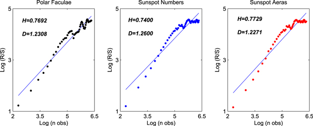
Figure 5. Log–log plots of R/S as a function of s for polar faculae (left panel), sunspot numbers (middle panel), and sunspot areas (right panel).
Download figure:
Standard image High-resolution imageMore importantly, the Hurst exponent H of a time series is directly related to its fractal dimension D, and the mathematical relationship between these two parameters is D = 2 − H (Das et al. 2009). The fractal dimension D is a statistical quantity that measures the dynamical complexity of the chaotic time series. Using this equation, the fractal dimensions are found to be 1.2308 ± 0.0525 for polar faculae, 1.2600 ± 0.0684 for sunspot numbers, and 1.2271 ± 0.0672 for sunspot areas. Our results suggest that both the high- and the low-latitude solar activity have distinctly fractal natures. Furthermore, the values of D show that the fractal nature of the solar activity is due to its long-range correlation.
After calculating the fractal dimensions D of the three time series, their corresponding predictability indicators P can be determined from the statistical relationship  If the value of P of a time series is close to zero, the considered system will be unpredictable. However, if the value of P becomes close to one, the dynamical system can be taken as a highly predictable process (Ghosh et al. 2014). Using this equation, the predictability indicators can be evaluated as 0.5384 ± 0.1050 for polar faculae, 0.4800 ± 0.1368 for sunspot numbers, and 0.5458 ± 0.1344 for sunspot areas, respectively. The P values of the three time series are around 0.5, indicating that the solar activity cycle is predictable in nature. It should be emphasized that the analysis results do not provide any concept on the predictable timescale. Subsequently, the method named the largest Lyapunov exponent is utilized to describe the dynamical complexity and to calculate the predictability timescale of the three time series.
3.2.2. Largest Lyapunov Exponent
A chaotic system is a deterministic system that is usually characterized by the fractal structure and sensitivity to small changes in initial conditions. The chaotic property of an attractor can be quantitatively described by many chaotic variables, such as the largest Lyapunov exponent, the correlation dimension, the Kolmogorov entropy, and so on (Hegger et al. 1999). In the Lyapunov exponent analysis (Eckmann et al. 1986), the quantities investigated are assumed to follow a set of differential equations in a high-dimensional phase space. These unknown equations are usually nonlinear and the apparent randomness of the generated series may reflect chaotic solutions of this set of nonlinear equations. The distance between two initially close orbits evolves exponentially, with a characteristic exponent λ, known as the Lyapunov exponent. The Lyapunov exponent is a measure of the rate at which nearby trajectories in phase space diverge. Moreover, it measures how predictable or unpredictable the system is. For chaotic orbits, there is at least one positive Lyapunov exponent. The positive Lyapunov exponent is a necessary condition for deterministic chaos but not sufficient. For periodic orbits, all Lyapunov exponents are negative. The Lyapunov exponent is zero near a bifurcation, which reflects the fact that the orbits evolve slower than exponentially.
The largest Lyapunov exponent, defined as the divergence of nearby trajectories in the phase space, is a convincing indicator to characterize the chaotic behavior and the dynamical complexity of a time series. Rosenstein et al. (1993) proposed an algorithm to calculate the largest Lyapunov exponent: after reconstructing the phase space, choose a point xno and all neighbor points xn, then calculate their average distance from that point, and finally estimate the average quantity S (stretching factor) by repeating the above procedures for N numbers of those points along the orbits:

where  is the number of neighbor points around xno. The plot of the stretching factors S versus the number of points N (or time interval t = NΔ t) will produce a curve with a rapid increase at the beginning and followed by a relatively flat region. Hegger et al. (1999) described the implementation of methods of nonlinear time series analysis, which are based on the paradigm of deterministic chaos and fractal behavior. A range of these algorithms has been made available in the form of computer programs by the TISEAN package8
(for details, see Hegger et al. 1999).
is the number of neighbor points around xno. The plot of the stretching factors S versus the number of points N (or time interval t = NΔ t) will produce a curve with a rapid increase at the beginning and followed by a relatively flat region. Hegger et al. (1999) described the implementation of methods of nonlinear time series analysis, which are based on the paradigm of deterministic chaos and fractal behavior. A range of these algorithms has been made available in the form of computer programs by the TISEAN package8
(for details, see Hegger et al. 1999).
In Figure 6, we plot the variations of the divergence as a function of the time interval for polar faculae (left panel), sunspot numbers (middle panel), and sunspot areas (right panel), respectively. From this figure, one can see that the profiles of the three curves display expected linear increases and relatively flat regions with some fluctuations superimposed on the part of the curves. The slopes (corresponding to the largest Lyapunov exponent for the three time series) are estimated through the least-squares line fitting method. We find that reasonable values of the largest Lyapunov exponent are 0.1429 ± 0.0304 month−1 for polar faculae, 0.0654 ± 0.0151 month−1 for sunspot numbers, and 0.1198 ± 0.0054 month−1 for sunspot areas. These positive values indicate the possible existence of chaotic behavior in the solar activity. This result is consistent with the estimation of a low-dimensional chaotic attractor from the phase-space reconstruction and the false nearest neighbor method, as already discussed above. According to the information theory method, the larger the largest Lyapunov exponent, the more complex the dynamical behavior of the system. Our results suggest that the dynamic behavior or the chaotic degree of the polar faculae and the sunspot areas is more complex than that of the sunspot numbers. The predictability timescale, defined as the inverse of the largest Lyapunov exponent, is taken as the length of the strange attractor. In this sense, the predictability timescales are calculated to be 0.6108 ± 0.1299 year for polar faculae, 1.3443 ± 0.3091 year for sunspot numbers, and 0.6996 ± 0.0.0552 years for sunspot areas. Therefore, the effective timescale used for forecasting the solar activity cycle is smaller than three years, i.e., the high-accuracy prediction of the solar magnetic activity should only be done for short- to mid-term due to its intrinsically dynamical complexity.

Figure 6. Variations of the divergence as a function of time interval for polar faculae (left panel), sunspot numbers (middle panel), and sunspot areas (right panel).
Download figure:
Standard image High-resolution image
3.2.3. Statistical Significance Test: Surrogate Data
Understanding the nonlinear behavior of a time series plays an integral role in the detection of deterministic chaos in physical systems (Schreiber & Schmitz 2000). One approach is to formulate a null hypothesis for a specific class of processes and compare the system output to this hypothesis. The surrogate data method is a classical way to establish such a null hypothesis and can be undertaken in two distinct ways. Typical realizations are Monte Carlo generated surrogate time series from a model that provides a suitable fit to the data; constrained realizations are surrogate time series generated from the data values to conform the certain properties of the data (Suzuki et al. 2007). The latter approach is more suitable for hypothesis testing as it does not require the definition of a pivotal test statistic (Theiler & Prichard 1996). Theiler et al. (1992) suggested some algorithms for generating surrogate data, such as the Fourier transform (FT) algorithm, the windowed Fourier transform algorithm, the amplitude-adjusted Fourier transform (AAFT) algorithm, and so on. In this paper, we generate 30 surrogate time series, using the AAFT algorithm, that have the same mean, variance, and autocorrelation function as the original time series. The AAFT algorithm can be described by the following three steps:
(1). We produce Gaussian random time series η(t) ∼ N(0,1) and shuffle the temporal order to obtain the same rank order as with the original time series X(i). Here, the rank order is defined as an order of state values of a time series (Suzuki et al. 2007). In this process, the shuffled time series ω(i) corresponds to a linear stochastic process and X(i) is considered to be a realization of a transformation of ω(i) through a static monotonic nonlinear function h( · ). That is, X(i) = h(ω(i)).
(2). Since the shuffled time series ω(i) is a realization that can be characterized by its power spectrum, we apply the FT algorithm to ω(i). The FT algorithm is as follows: the FT is applied to a target time series, in this case ω(i), and its power spectrum is obtained. Next, preserving a symmetry of phase components of the FT, the phase components are randomized. Then, the inverse FT generates an FT surrogate, which preserves the power spectrum of the target time series ω(i). Namely, in this process, we make an FT surrogate  of ω(i), which has exactly the same power spectrum as ω(i).
(3). We shuffle the original time series X(i) to obtain the same rank order as the FT surrogate time series  of ω(i) given in the previous step. Here, we again consider a static monotonic nonlinear function h( · ). Namely,
  =h(
=h( ), and
  is called the AAFT surrogate data version of X(i).
Based on the AAFT algorithm, we generate 30 surrogate time series each of polar faculae, sunspot numbers, and sunspot areas. We then calculate the Hurst exponents and the largest Lyapunov exponents of each time series, as shown in Tables 1 and 2. From Table 1, the average values of the 30 Hurst exponents are H = 0.7765 ± 0.0444 for polar faculae, H = 0.7786 ± 0.0496 for sunspot numbers, and H = 0.7945 ± 0.0491 for sunspot areas. Using the mathematical relationship among the Hurst exponent, the fractal dimension, and the predictability indicator, the fractal dimensions and the predictability indicators are calculated to be D = 1.2235 ± 0.0444 and P = 0.5530 ± 0.0888 for polar faculae, D = 1.2214 ± 0.0496 and P = 0.5572 ± 0.0992 for sunspot numbers, and D = 1.2054 ± 0.0491 and P = 0.5891 ± 0.0982 for sunspot areas. From Table 2 aj521731t2, the average values of the 30 largest Lyapunov xponents are 0.1148 ± 0.0292 month−1 for polar faculae, 0.0675 ± 0.0236 month−1 for sunspot numbers, and 0.0950 ± 0.0225 month−1 for sunspot areas. The predictability timescales are calculated to be 0.7761 ± 0.1974 year for polar faculae, 1.4065 ± 0.4918 year for sunspot numbers, and 0.9293 ± 0.2201 year for sunspot areas.
Table 1. Hurst Exponents of the 30 Surrogate Time Series Obtained Through the AAFT Algorithm of Polar Faculae, Sunspot Numbers, and Sunspot Areas
| No. | Polar Faculae | Sunspot Numbers | Sunspot Areas |
|---|---|---|---|
| 1 | 0.7161 ± 0.0562 | 0.7635 ± 0.0395 | 0.8205 ± 0.0397 |
| 2 | 0.7789 ± 0.0513 | 0.8945 ± 0.0388 | 0.7561 ± 0.0594 |
| 3 | 0.8039 ± 0.0297 | 0.7358 ± 0.0523 | 0.6639 ± 0.0753 |
| 4 | 0.8303 ± 0.0393 | 0.7523 ± 0.0470 | 0.7327 ± 0.0562 |
| 5 | 0.8402 ± 0.0290 | 0.8572 ± 0.0367 | 0.8537 ± 0.0372 |
| 6 | 0.7999 ± 0.0474 | 0.7083 ± 0.0603 | 0.8476 ± 0.0503 |
| 7 | 0.7884 ± 0.0422 | 0.7805 ± 0.0529 | 0.8534 ± 0.0333 |
| 8 | 0.8063 ± 0.0474 | 0.7722 ± 0.0539 | 0.7736 ± 0.0538 |
| 9 | 0.8217 ± 0.0307 | 0.8305 ± 0.0495 | 0.8133 ± 0.0562 |
| 10 | 0.6975 ± 0.0478 | 0.7089 ± 0.0693 | 0.8506 ± 0.0432 |
| 11 | 0.8117 ± 0.0360 | 0.6437 ± 0.0759 | 0.7230 ± 0.0494 |
| 12 | 0.7776 ± 0.0437 | 0.7404 ± 0.0584 | 0.8081 ± 0.0558 |
| 13 | 0.8131 ± 0.0456 | 0.7857 ± 0.0489 | 0.8155 ± 0.0438 |
| 14 | 0.8364 ± 0.0272 | 0.8376 ± 0.0414 | 0.8037 ± 0.0475 |
| 15 | 0.8535 ± 0.0354 | 0.7886 ± 0.0450 | 0.8067 ± 0.0417 |
| 16 | 0.7350 ± 0.0522 | 0.7855 ± 0.0427 | 0.8119 ± 0.0583 |
| 17 | 0.8213 ± 0.0371 | 0.7431 ± 0.0675 | 0.7442 ± 0.0724 |
| 18 | 0.7570 ± 0.0404 | 0.7892 ± 0.0473 | 0.8211 ± 0.0526 |
| 19 | 0.7907 ± 0.0406 | 0.7918 ± 0.0475 | 0.7686 ± 0.0524 |
| 20 | 0.7494 ± 0.0545 | 0.7513 ± 0.0614 | 0.7933 ± 0.0605 |
| 21 | 0.7163 ± 0.0587 | 0.7911 ± 0.0455 | 0.8384 ± 0.0436 |
| 22 | 0.7721 ± 0.0455 | 0.8309 ± 0.0476 | 0.7000 ± 0.0526 |
| 23 | 0.7686 ± 0.0416 | 0.7943 ± 0.0625 | 0.8122 ± 0.0479 |
| 24 | 0.7114 ± 0.0638 | 0.7447 ± 0.0575 | 0.8206 ± 0.0413 |
| 25 | 0.7624 ± 0.0529 | 0.7551 ± 0.0645 | 0.7436 ± 0.0594 |
| 26 | 0.7902 ± 0.0326 | 0.8079 ± 0.0500 | 0.8653 ± 0.0429 |
| 27 | 0.6836 ± 0.0570 | 0.8222 ± 0.0573 | 0.8072 ± 0.0458 |
| 28 | 0.7424 ± 0.0569 | 0.7821 ± 0.0489 | 0.7517 ± 0.0609 |
| 29 | 0.7658 ± 0.0450 | 0.8243 ± 0.0458 | 0.8042 ± 0.0410 |
| 30 | 0.7539 ± 0.0530 | 0.7449 ± 0.0652 | 0.8318 ± 0.0457 |
| Average | 0.7765 ± 0.0444 | 0.7786 ± 0.0496 | 0.7945 ± 0.0491 |
Download table as: ASCIITypeset image
Table 2. Largest Lyapunov Exponents of the 30 Surrogate Time Series Obtained Through the AAFT Algorithm of Polar Faculae, Sunspot Numbers, and Sunspot Areas
| No. | Polar Faculae | Sunspot Numbers | Sunspot Areas |
|---|---|---|---|
| 1 | 0.1107 ± 0.0080 | 0.0379 ± 0.0031 | 0.1027 ± 0.0076 |
| 2 | 0.0591 ± 0.0082 | 0.0333 ± 0.0025 | 0.0915 ± 0.0096 |
| 3 | 0.1277 ± 0.0311 | 0.0827 ± 0.0204 | 0.1094 ± 0.0037 |
| 4 | 0.0684 ± 0.0151 | 0.0587 ± 0.0080 | 0.0934 ± 0.0105 |
| 5 | 0.0692 ± 0.0033 | 0.0689 ± 0.0080 | 0.1071 ± 0.0022 |
| 6 | 0.0768 ± 0.0049 | 0.0609 ± 0.0072 | 0.0908 ± 0.0209 |
| 7 | 0.1146 ± 0.0135 | 0.0525 ± 0.0080 | 0.1108 ± 0.0020 |
| 8 | 0.1256 ± 0.0148 | 0.0694 ± 0.0033 | 0.1119 ± 0.0158 |
| 9 | 0.1340 ± 0.0197 | 0.0601 ± 0.0092 | 0.0685 ± 0.0128 |
| 10 | 0.1593 ± 0.0350 | 0.0545 ± 0.0046 | 0.0666 ± 0.0021 |
| 11 | 0.0988 ± 0.0027 | 0.0701 ± 0.0072 | 0.1196 ± 0.0317 |
| 12 | 0.0823 ± 0.0088 | 0.0623 ± 0.0089 | 0.1095 ± 0.0061 |
| 13 | 0.1159 ± 0.0093 | 0.0767 ± 0.0046 | 0.1192 ± 0.0048 |
| 14 | 0.1290 ± 0.0026 | 0.0814 ± 0.0113 | 0.0784 ± 0.0077 |
| 15 | 0.1314 ± 0.0326 | 0.0621 ± 0.0068 | 0.1282 ± 0.0077 |
| 16 | 0.1266 ± 0.0239 | 0.0379 ± 0.0035 | 0.1011 ± 0.0172 |
| 17 | 0.1077 ± 0.0233 | 0.0632 ± 0.0036 | 0.0979 ± 0.0054 |
| 18 | 0.1456 ± 0.0265 | 0.0654 ± 0.0071 | 0.1198 ± 0.0059 |
| 19 | 0.1502 ± 0.0356 | 0.0584 ± 0.0090 | 0.0646 ± 0.0031 |
| 20 | 0.1141 ± 0.0051 | 0.0913 ± 0.0033 | 0.0983 ± 0.0120 |
| 21 | 0.1686 ± 0.0157 | 0.1054 ± 0.0073 | 0.0700 ± 0.0136 |
| 22 | 0.1325 ± 0.0110 | 0.0767 ± 0.0088 | 0.1418 ± 0.0157 |
| 23 | 0.1207 ± 0.0106 | 0.0605 ± 0.0069 | 0.0689 ± 0.0031 |
| 24 | 0.1604 ± 0.0330 | 0.0450 ± 0.0068 | 0.0836 ± 0.0101 |
| 25 | 0.1089 ± 0.0082 | 0.0854 ± 0.0049 | 0.1024 ± 0.0185 |
| 26 | 0.0879 ± 0.0101 | 0.1411 ± 0.0108 | 0.0658 ± 0.0063 |
| 27 | 0.1207 ± 0.0067 | 0.0969 ± 0.0078 | 0.0745 ± 0.0071 |
| 28 | 0.1202 ± 0.0011 | 0.0463 ± 0.0058 | 0.1152 ± 0.0117 |
| 29 | 0.1137 ± 0.0151 | 0.0926 ± 0.0138 | 0.0929 ± 0.0073 |
| 30 | 0.0619 ± 0.0014 | 0.0272 ± 0.0038 | 0.0458 ± 0.0032 |
| Average | 0.1148 ± 0.0292 | 0.0675 ± 0.0236 | 0.0950 ± 0.0225 |
Download table as: ASCIITypeset image
All analysis results are summarized in Table 3. From this table, one can see that the analysis results obtained by the surrogate data method are very similar to those given by the above sections. Therefore, it is safe to say that the quantitative analysis results through the nonlinear time series analysis techniques used in this paper have a high degree of credibility. Based on the analysis results shown in Table 3, we make the following conclusions: (1) both the high- and the low-latitude solar activity show persistence on large scales and have distinctly fractal natures. Moreover, the fractal nature of the solar activity is due to its long-range correlation; (2) the solar magnetic activity cycle is predictable in nature, but the high-accuracy prediction should only be done for short- to mid-term due to its intrinsically dynamical complexity; and (3) the dynamical behavior or the chaotic degree of polar faculae is the most complicated, followed by sunspot areas, and then sunspot numbers because the largest Lyapunov exponent of polar faculae is the largest, which is in agreement with the results shown in the reconstructed phase spaces (Figure 4).
Table 3. Summary of Chaotic and Fractal Properties of Polar Faculae, Sunspot Numbers, and Sunspot Areas
| H | D | P | LLE | PTS | |
| SPF | 0.7692 ± 0.0525 | 1.2308 ± 0.0525 | 0.5384 ± 0.1050 | 0.1429 ± 0.0304 | 0.6108 ± 0.1299 |
| SSN | 0.7400 ± 0.0684 | 1.2600 ± 0.0684 | 0.4800 ± 0.1368 | 0.0654 ± 0.0151 | 1.3443 ± 0.3091 |
| SSA | 0.7729 ± 0.0672 | 1.2271 ± 0.0672 | 0.5458 ± 0.1344 | 0.1198 ± 0.0054 | 0.6996 ± 0.0552 |
| SSPF | 0.7765 ± 0.0444 | 1.2235 ± 0.0444 | 0.5530 ± 0.0888 | 0.1148 ± 0.0292 | 0.7761 ± 0.1974 |
| SSSN | 0.7786 ± 0.0496 | 1.2214 ± 0.0496 | 0.5572 ± 0.0992 | 0.0675 ± 0.0236 | 1.4065 ± 0.4918 |
| SSSA | 0.7945 ± 0.0491 | 1.2054 ± 0.0491 | 0.5891 ± 0.0982 | 0.0950 ± 0.0225 | 0.9293 ± 0.2201 |
Note. SPF: smoothed polar faculae; SSN: smoothed sunspot numbers; SSA: smoothed sunspot areas; SSPF: surrogate polar faculae; SSSN: surrogate sunspot numbers; SSSN: surrogate sunspot areas; H: Hurst exponent; D: fractal dimension; P: predictability indicator; LLE: largest Lyapunov exponent (in month−1); PTS: predictability timescale (in years).
Download table as: ASCIITypeset image
4. CONCLUSION AND DISCUSSION
Nonlinear analysis approaches enable us to learn more about the irregular behavior of the solar magnetic activity cycle. On the basis of the time series of polar faculae, sunspot numbers, and sunspot areas, we investigate the chaotic and fractal properties of both the high- and the low-latitude solar activity. First, we reconstruct the phase spaces of the three time series with the estimated parameters, i.e., the time delays and the embedding dimensions, which are calculated by the mutual information and the false nearest neighbor methods. Second, R/S analysis and the largest Lyapunov exponent are used to calculate the complexity indicators of each time series, including the Hurst exponents, the fractal dimensions, the predictability indicators, the largest Lyapunov exponents, and the predictability timescales. Finally, we apply the surrogate data method to generate 30 surrogate time series for each time series and re-calculate the above-mentioned statistical parameters. By means of the qualitative and quantitative analysis approaches, it is safe to say that the chaotic and fractal fractal properties of solar time series analyzed in this paper have a high degree of credibility. The remarkable conclusions are outlined as follows:
(1). The nonlinear dynamics underlying the solar magnetic activity (both the high- and low-latitude solar activity) should be governed by a three-dimensional chaotic attractor, and the chaotic behavior of polar faculae is the most complex, followed by sunspot areas, and then sunspot numbers.
(2). Both the high- and low-latitude solar activity could show a high degree of persistent behavior on large scales. Moreover, the fractal nature of the solar magnetic activity cycle is due to the long-range correlation.
(3). Although the solar magnetic activity cycle is predictable in nature, the high-accuracy forecast should only be done for a short- to mid-term timescale due to its intrinsically dynamical complexity.
Based on the Babcock–Leighton dynamo model, the solar magnetic fields with opposite polarity (Charbonneau 2014). The generation of toroidal magnetic fields is probably a rather deterministic and orderly process, whereas the generation of poloidal magnetic fields seems to be a complex process, as only a very small fraction (1%–2%) of the toroidal magnetic fields are converted to polar magnetic fields by turbulent diffusion and/or meridional circulation. Choudhuri (1992) argued that the stochastic fluctuations around the averages of various quantities in the dynamo process can be contributed to the irregularities of the solar magnetic activity cycle. Later, Jiang et al. (2007) and Choudhuri et al. (2007) identified the production of poloidal magnetic fields as the main source of randomness in the dynamo process because the convective buffeting on rising flux tubes causes a scatter in the tilt angles, whereas the other aspects of the dynamo process are assumed to be deterministic. Therefore, the nonlinear coupling of polar magnetic fields with the strong active-region fields exhibits a complex manner, causing the statistical similarities and differences (i.e., globally similar, but different in detail) between polar faculae and sunspot-related indices. More observations and/or theories of the nonlinear effect presented in the solar dynamo processes, including the stochastic fluctuations of the α−ω effect, the variation in the turbulent diffusion and/or the meridional circulation, the nonlinear back-reaction of the differential rotation, and the on–off intermittency of the nonlinear dynamo actions, are called for to address the physics of the nonlinear dynamical behavior precisely. These will improve the knowledge on the origin of the solar magnetic activity cycle and the temporal variation of solar magnetic fields.
The observational data of polar faculae were recorded on the sunspot sketches made with the Zeiss 20 cm refractor at Mitaka of the National Astronomical Observatory of Japan (http://solarwww.mtk.nao.ac.jp/en/db_faculae.html). The time series of sunspot numbers are downloaded from WDC-SILSO (World Data Center-Sunspot Index and Long-term Solar Observations) at the Royal Observatory of Belgium (http://www.sidc.be/silso). The time series of sunspot areas are taken from the Royal Greenwich Observatory (RGO) archive and the National Aeronautics and Space Administration (NASA) website (http://solarscience.msfc.nasa.gov/greenwch.shtml). This work is supported by the Specialized Research Fund for State Key Laboratories, the Chinese Academy of Sciences "Light of West China" Program, the Yunnan Science Foundation of China under grant No. 2015FB192, and the National Natural Science Foundation of China (NSFC) under grant Nos. U1531140, 41274176, 11503082, and 11463003. Last, but not least, the authors wish to express their gratitude to the anonymous referee(s) and the editor for meaningful suggestions and requests that greatly improved the original draft.
Footnotes
- 5
- 6
- 7
- 8