

Abstract
Concentrator photovoltaics (CPV) can efficiently convert light into electricity; however, conventional CPVs require large and heavy tracking systems. Microtracking CPVs (MTCPVs) can solve this significant problem. Most MTCPV systems have a limited angle of incidence (AOI). If diffuse light was used, MTCPV required traveling light from top to bottom. In this study, a spherical-lens-based microtracking CPV (SMTCPV) with a pin-type second optical element (SOE) was developed. In SMTCPV, the light travel light from above to below. Pin-type SOEs were inserted between the spherical lenses, thus increasing the acceptable wide AOI. Optical analysis and calculations of the interaction between overlapping spherical lenses and pin-type SOEs were performed. An optical efficiency of 59% was maintained at any angle when the gap was considered. The maximum AOI was 64.7° in the direction of adjacent spherical lenses and 90° in the gap direction.
Export citation and abstract BibTeX RIS
1. Introduction
Fossil fuels will be exhausted within 200 years; however, the Earth receives 170 billion MW of solar energy in every year. Photovoltaics can convert this enormous amount of solar energy into usable electrical energy. 1) Single-junction solar cells approach the Shockley–Kuisser limit of 32%–33%, but multijunction solar cells can exceed this limit because of the stacking of photovoltaic materials with an appropriate bandgap. 2) Concentrator photovoltaics (CPVs) increase the conversion efficiency by several hundred times with a metal grid geometry 3) and reduce the cost of smaller solar cells. A cell efficiency of 47.1% has been achieved. 4) Using lens focusing and field measurements, a module efficiency of 36.7% has been achieved. 5) High concentrations can achieve a high conversion efficiency.
However, three problems are associated with high-concentrator photovoltaics: (i) High-concentrator photovoltaics can only convert direct light, (ii) solar tracking is required to concentrate the light, and (iii) an acceptably wide angle of incidence (AOI) is required. Two solutions have been proposed to solve this problem, in which only direct light can be converted: (1) diffuse light, which is not direct light, is transmitted to the concentrator photovoltaic (transmitted CPV) and used for other purposes, such as agriculture. 6) (2) Hybrid multijunction solar cells (hybrid CPV) are hybrids of multi-junction solar cells with concentrator and Si solar cells without concentrator. Direct light is concentrated and converted using the multijunction solar cells. Diffuse light is converted using Si solar cells. 7) Solutions using (1) transmitted CPVs and (2) hybrid-type CPVs require a structure in which light travels from top to bottom within the CPV.
Conventional solar-tracking systems are large and heavy. Several microtracking CPV (MTCPV) systems have been proposed to address this significant problem. 8) Previous MTCPV studies have investigated the following: (A) waveguide and lens structures on top of multijunction solar cells; (B) upper and lower mirrors on a multijunction solar cell structure; 9,10) and (C) a three-dimensional controlled structure of a solar cell stage and an acceptably wide AOI lens.
Type (A) structures were studied in the following ways: (a) modifying the lower waveguide shape (e.g. horizontally tapered waveguide, 11) branched planar waveguide, 12) horizontally staggered light guide, 13) lens-channel waveguide, 14) staggered-tapered light guide 15)); (b) modifying the waveguide reflector (e.g. small lateral shifts of the waveguide, 16) horizontally spectrally separated waveguides 17)); (c) combining an external seasonal tracker; 18) (d) adding optical elements between the lens and the waveguide (e.g. bio-inspired curved light guide 19)); and (e) adding two-lens structures in the upper structure of a multijunction solar cell. 20,21) As light travels from top to bottom in the (A)-type tracker, this tracker can be applied as (1) a transmitted CPV and (2) a hybrid-type CPV. However, the AOI is restricted by the waveguide and lens conditions.
Type (B) structures have an acceptably wide AOI. However, this type of structure cannot be applied as a (1) transmitted CPV or (2) hybrid-type CPV because it uses an undermirror and light does not travel from top to bottom.
Type (C) structures use acceptably wide AOI lenses and movement mechanisms (e.g. horizontal and vertical displacement, 22) molded glass array lens, 23) ball guide support microtracking 24)). Theoretically, a spherical gradient index lens 25) and solar cell stage 26) have been proposed. Hybrid-type CPVs 27) and transmitted CPVs 28) have been proposed because of their structure, in which light travels from top to bottom. However, the AOI is limited by the interference between the spherical lens and the solar cells.
In this study, a structure consisting of a spherical lens MTCPV (SMTCPV) and pin-type second optical element (SOE) was adopted as Type (C). The spherical lens had a focal point from any AOI without rotation 29) and an acceptably wide AOI lens. Our SMTCPV is applicable to transmitted and hybrid CPVs, where light travels from top to bottom. Solar tracking can only be performed with horizontal and vertical movements without rotation using a spherical lens. The overlap radius of the spherical lenses can be adjusted to achieve a wider maximum AOI and higher optical efficiency. The distance between the spherical lenses was varied and analyzed to resolve the interaction between the spherical lenses and the pin-type SOEs.
2. Concept of SMTCPV with pin-type SOEs
Figures 1(a) and 1(b) show the light incident on the SMTCPV without pin-type SOEs in the vertical direction (AOI = 0°) and inclined direction, respectively. Figures 1(c) and 1(d) show light incident on the SMTCPV with pin-type SOEs in the vertical direction (AOI = 0°) and inclined direction, respectively. A spherical lens has a focal point at all AOIs. The solar cells were placed at the focal point below the lens when the Sun was directly above it (AOI = 0°). When light was incident from an inclined direction, as shown in Fig. 1(b), the lens moved vertically and the solar cells moved horizontally, placing the solar cells at the focal point. These relative movements enabled the SMTCPV to perform solar tracking without lens rotation. However, interference between the spherical lens and the solar cell stage restricts the maximum AOI  We added pin-type SOEs to the SMTCPV as shown in Figs. 1(c) and 1(d). Solar cells were placed at the bottom of the SOEs. The SOEs were placed at the focal point below the lens when the Sun was directly above the lens (AOI = 0°). When light was incident from an inclination angle, the cones of the SOEs were placed at a focal point. In particular, when the tilt angle was large, the upper SOEs were positioned between the lenses.
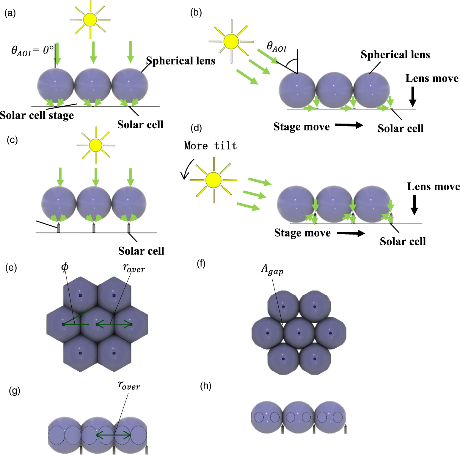
Fig. 1. Tracking motion and lens array. (a) SMTCPV without pin-type SOE at  (b) SMTCPV without pin-type SOE, irradiated from an inclined direction. (c) SMTCPV with pin-type SOE at
  (d) SMTCPV with pin-type SOE, irradiated from an inclined direction. (e) Lens array of
  top view. (f) Lens array of
  side view. (g) Lens array of
  top view. (h) Lens array of
  side view.
Download figure:
Standard image High-resolution imageTwo methods were proposed for three-dimensional (3D) mechanical control. (1) The solar cell stage moves laterally (XY-direction) and the spherical lens array moves vertically (Z-direction). 29) (2) Long-hole guides/pins on gears enable the lateral (XY-direction) movement of solar cells, whereas ball feet/guides passively enable the vertical (Z-direction) movement of solar cells. 24)
Thus, even when the focal point is between the spherical lenses, the maximum AOI can be increased by guiding Sunlight to the solar cells via the pin-type SOEs.
Figure 1(e) shows the top view of the lens array showing the closest packed state. Figure 1(f) shows the top view of the lens array with less overlap. Figure 1(g) shows a side view of the lens array showing the closest packed state. Figure 1(h) shows a side view of the lens array with minimal overlap. An overlap radius  was introduced to explain the overlap of the spherical lenses. The distance between the center of the spherical lens and the adjacent center is the overlap radius
  normalized by the spherical lens radius.
  is the director angle.
  is the direction from the spherical lens center to the adjacent spherical lens center, and
  is the direction from the spherical lens center to the gap between the three spherical lenses.
  is the gap between the three spherical lenses. The overlap radius at the closest packing is
  in Figs. 1(e) and 1(g), and the nonoverlapping but contacting condition is
  The overlap radii in Figs. 1(g) and 1(h) are
  Figure 1(g) shows that the maximum AOI is reduced when the overlap radius is small because pin-type SOEs are not inserted between the spherical lenses. However, as shown in Fig. 1(h), with an overlap radius
  pin-type SOEs can be inserted between spherical lenses, resulting in fewer overlapping spherical lenses and a wider maximum AOI.
3. Optical efficiency when the angle of incidence and shape of SOE are varied
Figure 2(a) illustrates the spherical lens and the upper part of the pin-type SOE at the top of the simulation model. Table I presents the simulation conditions. A spherical lens with a lens radius  mm is on the upper side, and a receiver and SOE are on the lower side. The SOE is cone-shaped with a height
  mm and the receiver bottom radius is
  mm. The material used is high RI epoxy considering a previous study.
30) The receiver varied the focusing distance along the z-axis, the x-axis was perpendicular to the focusing distance direction, and the rotation angle was perpendicular to the y-axis. A 3D ray-tracing analysis was performed using the commercial software from BestMedia Inc. The 3D ray-tracing analysis was performed by considering the Fresnel reflection losses and neglecting the volume absorption of the lens.
mm. The material used is high RI epoxy considering a previous study.
30) The receiver varied the focusing distance along the z-axis, the x-axis was perpendicular to the focusing distance direction, and the rotation angle was perpendicular to the y-axis. A 3D ray-tracing analysis was performed using the commercial software from BestMedia Inc. The 3D ray-tracing analysis was performed by considering the Fresnel reflection losses and neglecting the volume absorption of the lens.
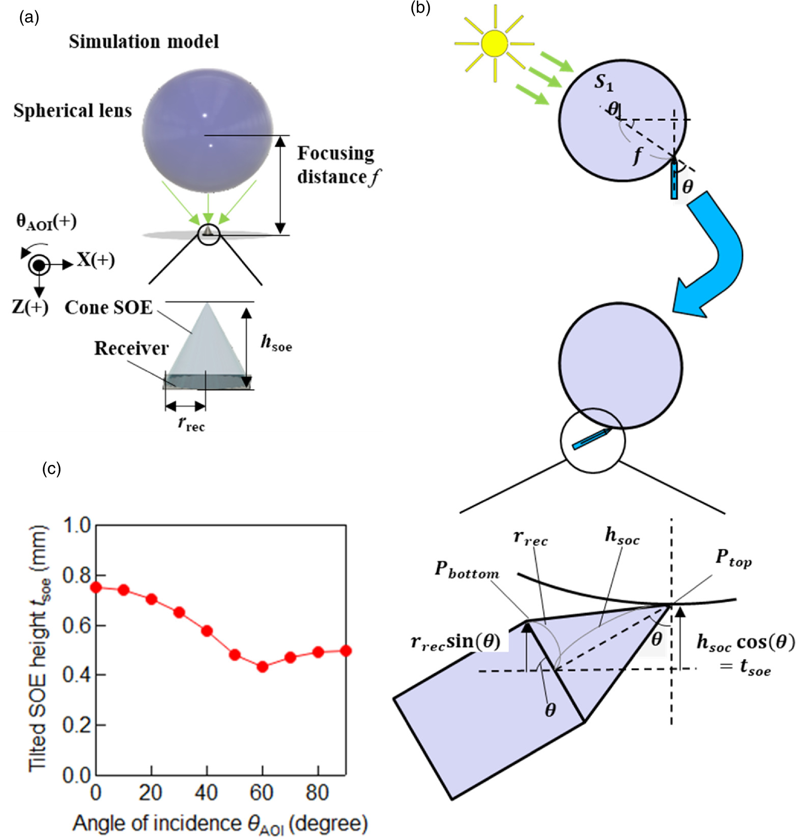
Fig. 2. Spherical lens and cone SOE. (a) Simulation model of spherical lens and cone SOE. (b) Schematic of cone SOE thickness  (c) Calculated tilted SOE height
  .
.
Download figure:
Standard image High-resolution imageTable I. Simulation conditions I.
| Spherical lens RI (PMMA) | 1.491 @ 587.6 nm 31) |
| SOE RI (Epoxy) | 1.589 @ 589 nm 32) |
| Lens radius rlens | 5 mm |
| Receiver bottom radius rrec | 0.5 mm |
| Receiver bottom shape | Rectangle 1 × 1 mm |
| Focusing distance f | 5–8 mm |
| SOE height hsoe | 0.75 mm, no SOE |
AOI 
| 0°–90° |
| Geometrical concentration ratio C | 78.5× |
| Ray spectrum | 750–949 nm (middle junction wavelength of the triple-junction solar cells) |
As pin-type SOEs are inserted between spherical lenses, SMTCPVs with pin-type SOEs are preferred because of their short focal distances. However, the spherical lens RI should consider the interference between the spherical lenses and the pin-type SOEs. In other simulations, The spherical lens in  which similar to RI of polymethyl methacrylate (PMMA) has the highest optical efficiency at
  mm which means
  Thus the PMMA lens is not interfere with the SOE. Therefore, PMMA was used for the spherical lens.
Figure 2(b) illustrates the thickness  of the cone SOE. The cone SOE has two ends: the cone SOE top end
  and the cone SOE bottom end
  The top end of the cone SOE is rotated from the receiver center as follows:
  The bottom end of the cone SOE is rotated from the receiver center as follows:
  The larger value between
  and
and  is the thickness of the cone SOE
  Figure 2(c) shows the relationship between
  and
and  with
with  mm and
  mm.
mm.
Figure 3 shows the optical efficiency maps with a cone SOE with  mm and without an SOE at each AOI; Z = 5 mm indicates that the receiver is placed on the surface of a spherical lens. The yellow line indicates the closest line that allows a cone SOE considering the cone SOE thickness
  as shown in Fig. 2(c).
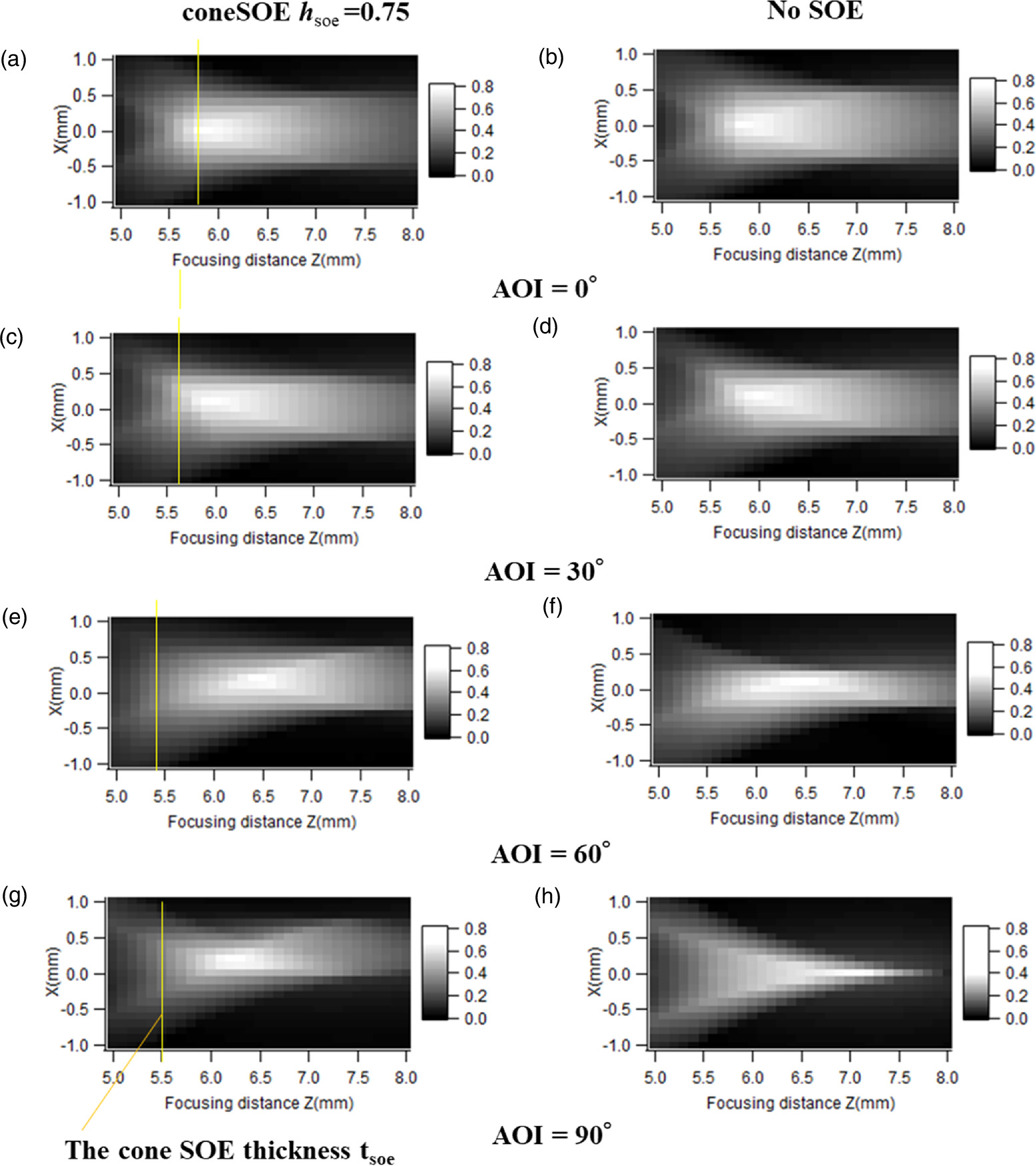
Fig. 3. Optical efficiency maps under the simulation conditions I. (a)  mm cone SOE and AOI = 0°, (b) no SOE and AOI = 0°, (c)
  mm cone SOE and AOI = 30
 (d) no SOE and AOI = 30°, (e)
  mm cone SOE and AOI = 60°, (f) no SOE and AOI = 60°, (g)
  mm cone SOE and AOI = 90
 (h) no SOE and AOI = 90°.
Download figure:
Standard image High-resolution imageTable II lists the optical efficiency of the point with the highest optical efficiency with an SOE and the optical efficiency of the same point without an SOE. The optical efficiency with an SOE is higher than that without an SOE; for  and
and  as the AOI is increased, the optical efficiency with the SOE is higher than that without the SOE. As shown in the optical efficiency map in Fig. 3, the white area, which indicates a high optical efficiency, is reduced under high-AOI conditions without the SOE.
Table II. Optical efficiency under the simulation conditions I.
| AOI | Z (mm) | X (mm) | With SOE optical efficiency (%) | Without SOE optical efficiency (%) |
|---|---|---|---|---|
| 0 | 5.8 | 0 | 77.5 | 75.0 |
| 10 | 5.9 | 0 | 75.1 | 73.9 |
| 20 | 5.9 | 0.1 | 74.0 | 72.3 |
| 30 | 6.0 | 0.1 | 71.3 | 70.9 |
| 40 | 6.2 | 0.1 | 67.0 | 66.3 |
| 50 | 6.4 | 0.1 | 66.5 | 60.7 |
| 60 | 6.4 | 0.2 | 62.3 | 45.5 |
| 70 | 6.4 | 0.2 | 59.8 | 26.8 |
| 80 | 6.4 | 0.2 | 61.6 | 22.3 |
| 90 | 6.2 | 0.2 | 66.4 | 30.0 |
Figure 4 shows the ray distribution points with and without the SOE in Table II. Figures 4(a) and 4(b) show the ray distributions at  Figures 4(c) and 4(d) shows the ray distributions at
  Figures 4(e) and 4(f) show the ray distributions at
  Figures 4(a), 4(c), and 4(e) show the ray distributions with the SOE. Figures 4(b), 4(d), and 4(f) shows the ray distributions without the SOE. Figures 4(a) and 4(b) show the circular ray distributions. Figure 4(d) shows the ray distribution at
  without the SOE. The ray distribution is elliptical owing to spherical aberration. Figure 4(c) shows the ray distribution at
  with the SOE. The ray distribution is also elliptical, and the light ray distribution is caused by reflections from the SOE walls. Figure 4(f) shows the ray distribution for
  without the SOE. The optical efficiency was reduced because the elliptical rays exceeded the measurement area. Figure 4(e) shows the ray distribution at
  with the SOE. The number of reflected rays increased, covering the area. Hence, the optical efficiency increased compared with that without the SOE. Simulations were performed at the bottom of the cone SOE. When a pole was added, the ray was dispersed at the bottom of the pole.
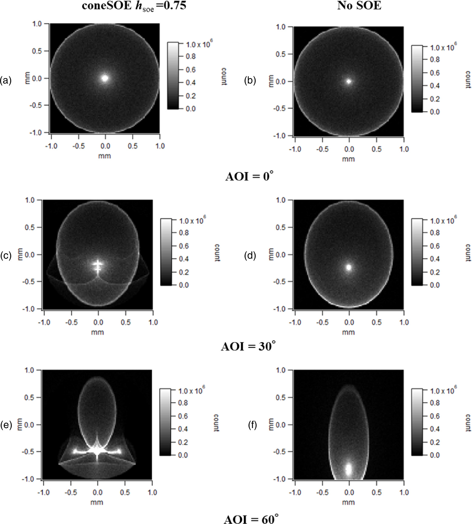
Fig. 4. Ray distributions under the simulation conditions I. (a)  mm cone SOE and AOI = 0
 (b) no SOE and AOI = 0°, (c)
  mm cone SOE and AOI = 30
 (d) no SOE and AOI = 30°, (e)
  mm cone SOE and AOI = 60°, (f) no SOE and AOI = 60°, (g)
  mm cone SOE and AOI = 90
 (h) no SOE and AOI = 90°.
Download figure:
Standard image High-resolution imageTable III lists the simulation condition considering the light ray spectrum of the multijunction solar cell. The energy generation by multijunction solar cells requires the consideration of the spectrum match between each subcell. The optical efficiency maps of each subcell at  and
and  are shown in Fig. 5. Figures 5(a) and 5(b) show the optical efficiency maps of the top subcell. Figures 5(c) and 5(d) show the optical efficiency maps of the middle subcell. Figures 5(e) and 5(f) shows the optical efficiency maps of the bottom subcell. Figures 5(a), 5(c), and 5(e) show the optical efficiency maps for
  Figures 5(b), 5(d), and 5(f) show the optical efficiency maps for
  Table IV presents the optical efficiency at the point with the highest optical efficiency for the middle subcell. Figure 5 shows that the focusing distance difference between the top, middle, bottom subcells is less than 0.2 mm. Table IV shows that the difference in the optical efficiency at the highest optical efficiency point in middle sub-cell is less than 1%. In this study, spherical lenses were used and the focusing distance of the spherical lenses was short. Therefore, the effect of chromatic aberration was smaller.
Table III. Simulation conditions II.
| Spherical lens RI (PMMA) | 1.491 @ 587.6 nm 31) |
| SOE RI (Epoxy) | 1.589 @ 589 nm 32) |
| Lens radius rlens | 5 mm |
| Receiver bottom radius rrec | 0.5 mm |
| Receiver bottom shape | Rectangle 1 × 1 mm |
| Focusing distance f | 5–8 mm |
| SOE height hsoe | 0.75 mm |
AOI 
| 0°–90° |
| Geometrical concentration ratio C | 78.5× |
| Ray spectrum | 280–749 nm (top junction) |
| 750–949 nm (middle junction) | |
| 950–2000 nm (bottom junction) | |
| (In triple-junction solar cells) |
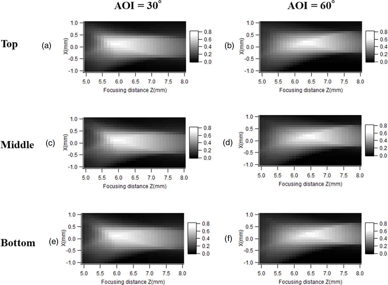
Fig. 5. Optical efficiency maps with different junctions in the triple-junction cell. (a) Top junction (280–749 nm) and AOI = 30 (b) Top junction and AOI = 60°, (c) Middle junction (750–949 nm) and AOI = 30
 (d) Middle junction and AOI = 60°, (e) Bottom junction (950–2000 nm) and AOI = 30
 (f) Bottom junction and AOI = 60°.
Download figure:
Standard image High-resolution imageTable IV. Optical efficiency under the simulation conditions II.
| AOI | Z (mm) | X (mm) | Top junction optical efficiency (%) | Middle junction optical efficiency (%) | Bottom junction optical efficiency (%) |
|---|---|---|---|---|---|
| 0 | 5.8 | 0 | 77.0 | 77.5 | 77.4 |
| 10 | 5.9 | 0 | 74.9 | 75.1 | 75.3 |
| 20 | 5.9 | 0.1 | 73.4 | 74.0 | 73.9 |
| 30 | 6.0 | 0.1 | 70.7 | 71.3 | 71.6 |
| 40 | 6.2 | 0.1 | 66.5 | 67.0 | 67.5 |
| 50 | 6.4 | 0.1 | 64.0 | 66.5 | 65.0 |
| 60 | 6.4 | 0.2 | 61.6 | 62.3 | 62.2 |
| 70 | 6.4 | 0.2 | 59.6 | 59.8 | 56.6 |
| 80 | 6.4 | 0.2 | 61.7 | 61.6 | 61.3 |
| 90 | 6.2 | 0.2 | 66.4 | 66.4 | 66.3 |
4. Overlapping radius and angle limit
We introduce numerical equations for the maximum AOI. Figures 6(a)–6(c) show a schematic of a spherical lens and a pin-type SOE when expanded to an angle other than  Figure 6(a) presents an overview. Figure 6(b) illustrates the angular schematic in the horizontal plane through the center
  of spherical lens S1 and the center
  of spherical lens S2. Figure 6(c) shows the angular schematic in the vertical plane between
  and the
  direction. The center of the spherical lens S2, when cut in the
  direction plane, is
  The slice overlap radius of S2 is
  The distance
  between
  and
and  is given by

The vertical distance  from
from  to
to  is given by

The sliced circle radius  is the radius cut in the
  direction of the spherical lens S2, and is given as follows. The radius of the spherical lens
  was 1.

[In Fig. 6(c), the focusing distance projection, where  is projected onto the line connecting
  and
and  is as follows.
These formulas use the normalized focal length  which is the focal length
  normalized by the lens radius
  The complementary maximum AOI
  of the sliced circle cut in the
  direction is given by
The maximum AOI  when the sliced circle is cut in the
  direction is given by

Fig. 6. Interference between the spherical lenses and the SOE. (a) Overview of the lens array. (b) Top view of the lens array. (c) Side view of the lens array. (d) Maximum AOI  with varying overlap radius
  at
at  (e) Maximum AOI
  with varying director angle
  for
for  .
.
Download figure:
Standard image High-resolution imageFigure 6(d) shows the relationship between the overlap radius and the maximum AOI at  The maximum AOI
  was
was  at the overlap radius
  at
at  However, at
  = 1.1, the maximum AOI was
  The maximum AOI can be increased by shortening the focusing distance. When the spherical lens overlap was reduced and the overlap radius was set to
  at
at  = 1.1, the maximum AOI was
  Figure 4(e) shows the maximum AOI
  when the directional angle
  and the overlap radius
  are varied. The closest focusing distance
  mm for a spherical lens radius
  mm and SOE thickness
  mm, which gives the closest normalized focusing distance
  There was interference between the spherical lenses and the pin-type SOEs, limiting the maximum AOI with the closest packing to
 at
at  and
and  at
at 
The shorter the overlap between the spherical lenses, the larger the  and the wider the distance between the spherical lenses. A gap occurred between the three spherical lenses centered at
  As the distance increased and gaps appeared, the maximum AOI also increased. At overlap radius
  = 1.9,
  at
at  and
and  at
at 
 indicates that a pin-type SOE can be inserted into the horizontal plane of the lens array. Therefore, the maximum AOI can be increased by reducing the spherical lens overlap and using a pin-type SOE. However, the shortening of the overlap of the
The gap area  and cover area ratio
  in the horizontal plane of the lens array are illustrated in Figs. 4(a)–4(c).
Figure 7(a) shows a schematic of the three spherical lenses. The three spherical lenses are denoted as S1, S2, and S3. S1, S2, and S3 are named Si or Sj or Sk using iterators i = 1, 2, 3 or j = 1, 2, 3 or k = 1, 2, 3. The centers of these lenses are 
 and
and  respectively. The horizontal plane of the lens array was rotated about the
  axis, and the state of the lens array was calculated with varying AOI.
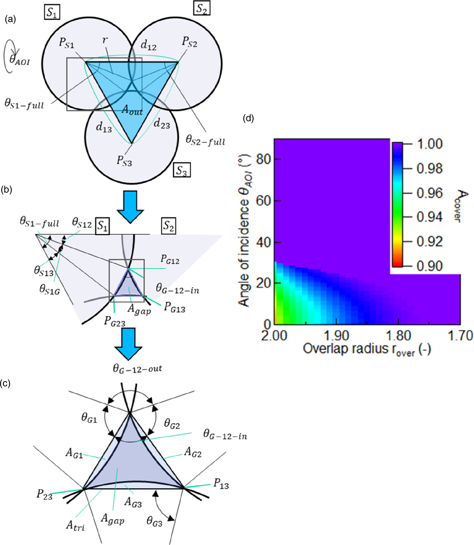
Fig. 7. Three spherical lenses and the gap. (a) Schematic of the three spherical lenses. (b) Schematic of the spherical lens S1 and gap. (c) Gap schematic (d) cover area ratio.
Download figure:
Standard image High-resolution imageThe distance between  and
and  is
is  which is given as follows:

The distance between  and
and  is
is  and that between
  and
and  is
is  which are given as follows:

The distance between other centers of these lense are named  using iterators i = 1, 2, 3 or j = 1, 2, 3. The same also applied to
  The Si full angle
  consists of the lines
  and
and  as follows.
The area of the triangle with  connected to
  is expressed below.

Figure 7(b) shows a schematic of the spherical lens S1 and the gap. This figure illustrates S1 as i = 1; however, S2 can also be discussed with i = 2 and S3 with i = 3.  is the gap vertex point between the spherical
  and
and  sides. The Si side angle
  consisting of the lines
  and
and  is given as follows.
The gap target angle  consists of
  and
and  as follows.

Figure 7(c) shows a schematic of the gap between the three spherical lenses. The gap outside angle  consists of
  and
and  as follows.

The gap side angle  consists of
  and
and  as follows.

The gap inside angle  consists of
  and
and  as follows.

Next, we describe this area. Subtracting the three fan sections  from the gap triangle area
  which consists of
  yields
The fan section area  is given as follows.

The gap triangle area  is given as follows.

The gap area  is given as follows.

The cover area ratio  is given as follows.
Figure 7(d) shows the cover area ratio  for varying overlap radius
  and AOI
 is smallest at
  = 2 when the spherical lenses do not overlap. On the other hand,
  is 1 at
  when the lens is the closest packed.
5. Optical efficiency considering SOE and overlapping radius
The modified optical efficiency  is calculated using the optical efficiency
  and cover area ratio
  as follows.

The optical efficiency  is obtained from Table II. The cover area ratio
  was selected from the overlap radius
  = 1.9 in Fig. 7(d).
The cover area ratio  was obtained from Fig. 7(d) for the overlap radius
  = 1.9.
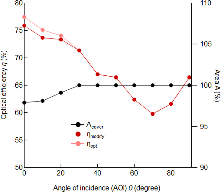
Figure 8 shows the optical efficiency with varying AOI for the overlap radius  and
and  The optical efficiency was 59.8% at the lowest
  indicating that the SMTCPV maintains a high efficiency over a wide range of AOI. Thus, a wide AOI
  and high optical efficiency can be achieved by introducing pin-type SOEs and adjusting the overlap radius
  After preparing the suitable samples, the actual conversion efficiencies were measured.
Fig. 8. Optical efficiency with varying AOI for overlap radius  and
and  .
.
Download figure:
Standard image High-resolution image
6. Conclusions
A spherical lens can focus light from any AOI to any point and can contribute to an SMTCPV system. We introduced a pin-type SOE and adjusted the spherical lens overlap radius to achieve a maximum AOI and high optical efficiency. Formulas were developed to calculate the maximum AOI considering the interference between the pin-type SOE and the solar cell stage. We also calculated the loss equation owing to the gap when the overlap radius of the spherical lens was varied to increase the maximum AOI. When the spherical lens overlap was adjusted to the overlap radius  = 1.9, the optical efficiency
  was maintained at 62.2% at
  Therefore, a larger maximum AOI and higher optical efficiency at wide angles can be achieved by introducing pin-type SOEs and varying the spherical lens overlap. In this study, the concentration ratio was maintained constant at 78.5 times. Previous studies have shown that core–shell spherical lenses have acceptable focusing distances and high optical efficiency.
29) Changing the light concentration ratio and using core–shell spherical lenses may improve the optical efficiency at all angles. In the future, all energy flow rates and conversion efficiencies will be calculated and realized as modules.
Therefore, a larger maximum AOI and higher optical efficiency at wide angles can be achieved by introducing pin-type SOEs and varying the spherical lens overlap. In this study, the concentration ratio was maintained constant at 78.5 times. Previous studies have shown that core–shell spherical lenses have acceptable focusing distances and high optical efficiency.
29) Changing the light concentration ratio and using core–shell spherical lenses may improve the optical efficiency at all angles. In the future, all energy flow rates and conversion efficiencies will be calculated and realized as modules.
Acknowledgments
The authors would like to thank Professor Hideo Fujikake of Tohoku University for insightful discussions.