Abstract
The most-studied classes of exact solutions to Vlasov–Maxwell equations for stationary neutral current structures in a collisionless relativistic plasma, which allow the particle distribution functions (PDFs) to be chosen at will, are reviewed. A general classification is presented of the current sheets and filaments described by the method of invariants of motion of particles whose PDF is symmetric in a certain way in coordinate and momentum spaces. The possibility is discussed of using these explicit solutions to model the observed and/or expected features of current structures in cosmic and laboratory plasmas. Also addressed are how the magnetic field forms and the analytical description of the so-called Weibel instability in a plasma with an arbitrary PDF.
Export citation and abstract BibTeX RIS
| V V Kocharovsky Institute of Applied Physics, Russian Academy of Sciences, ul. Ul'yanova 46, 603950 Nizhny Novgorod, Russian Federation; Department of Physics and Astronomy, Texas A&M University, College Station, TX 77843-4242, USA |
| E-mail: kochar@appl.sci-nnov.ru |
| Vl V Kocharovsky, V Yu Martyanov, S V Tarasov Institute of Applied Physics, Russian Academy of Sciences, ul. Ul'yanova 46, 603950 Nizhny Novgorod, Russian Federation |
1. Introduction. Magnetic fields in a collisionless plasma and Weibel instability
1.1. Objective of this review
Quasistationary magnetic fields maintained by intrinsic currents in a plasma determine to a large extent its kinetic, dynamic, and radiative properties. This phenomenon is especially apparent in collisionless neutral structures, where such fields are responsible for interactions between particles and are correlated with the local anisotropy of particle distribution. The energy distribution of particles may be far from a Maxwellian one in different physical conditions prevailing in both, cosmic and laboratory (including laser) plasmas. Despite the lack of quantitative data, results of in situ observations, laboratory experiments, and numerical simulations have one thing in common: they all suggest the existence in a collisional plasma of various long-lived (quasistationary) current structures considerably different in terms of particle distribution anisotropy, energy distribution of particles, spatial configuration of the current density, and magnetic fields generated by the current.
Numerous publications report attempts to kinetically describe magnetostatic self-consistent structures in a collisionless plasma [1–36]. Most of them refer to analytical studies, because numerical simulation does not yet provide a general approach to the solution to this complicated nonlinear problem. Unfortunately, many authors confine themselves to considering a very limited set of anisotropic particle distributions (usually a shifted Maxwellian distribution), which leaves only a narrow choice of spatial current density distributions. The few studies that allow an arbitrary particle distribution over energies and/or arbitrary spatial current profiles fail to provide a clear understanding of possible types of self-consistent current structures and their characteristic properties [14, 22, 27, 37].
A consistent analytical theory of self-consistent current structures in a collisionless plasma with arbitrary energy distribution of particles has only recently attracted the serious attention of researchers, with the most interesting results obtained by our method based on the invariants of particle motion and allowing the general case of relativistic multicomponent strongly anisotropic plasma to be analyzed [38].
The present review is the first one in this area of plasma physics; it encompasses the majority of the currently known classes of stationary analytical solutions of self-consistent Maxwell equations and kinetic equations of particle motion. It includes planar layered, cylindrically symmetric, and two-dimensional structures with a variety of current and magnetic field profiles, both localized and nonlocalized, rigorously taking into account the complicated motion of trapped and transit particles and the spatial nonuniformity of the anisotropy of their distribution function. An analytical description of a number of possible current structures at the boundary between a nonmagnetized plasma and a plasma in a strong external magnetic field is presented. The large number of exact solutions for special particle distribution functions (PDFs) makes practically impossible a detailed discussion of all available solutions in the framework of a single review. We rely on the understanding of those authors whose data remained beyond the scope of this review; moreover, it does not include all our own results.
The review is focused on the comparative analysis of the most representative solutions with reference to their application for the construction of analytical models of various current configurations in cosmic and laboratory plasmas, and for the interpretation of results of numerical simulations of collisionless plasma dynamics. To make the picture complete, the Introduction includes a concise analysis of Weibel type instability that strongly depends on PDFs and may be responsible for the formation or destruction of current structures. In addition, Section 4.4 contains data on certain specific features of the anisotropy of synchrotron radiation spectra from self-consistent current sheets that have recently been clarified due to exact solutions for structures with the polynomial PDFs.
1.2. Magnetic field problem in a collisionless plasma
The problem of the formation and prolonged occurrence of the magnetic field in a nonequilibrium weakly collisional plasma has remained in the focus of attention over decades (see, for instance, reviews [39–46]).
This problem includes, besides an analysis of the development and saturation of Weibel type instabilities responsible for generating a magnetic field, the solution to the complicated nonlinear problem of possible quasistationary current structures consistent with their inherent and/or external magnetic field. Such structures can qualitatively alter the particle and field dynamics in a plasma and thereby its kinetic and dynamic properties at large. Investigations in this area are especially topical for the study of strongly nonequilibrium plasmas, e.g., explosive phenomena in astrophysical objects, active regions of solar and planetary magnetospheres, or the ejection of matter from targets irradiated by strong laser beams.
Considerable progress in solving this problem has thus far been achieved only in the magnetohydrodynamic approximation that holds true for a sufficiently dense plasma and structures with scales much larger than the mean free path of a particle [43, 47, 48]. For smaller-scale structures, i.e., rarefied or so-called collisionless plasma, only scattered data are available [9, 40–42, 49–54], which do not provide a complete understanding of the mechanisms underlying collective interactions among particles via the intricately structured magnetic field they generate. This field is involved in practically all essential phenomena occurring in a collisionless plasma, such as the formation of collisionless shock waves, the reconnection of magnetic tubes of force, particle acceleration in various stratified plasma flows, the formation of mutually consistent radiation spectra and PDFs. Solving such problems inevitably requires an analysis of the structure of a self-consistent magnetic field in the plasma with a rather arbitrary energy distribution of particles.
A description of the possible diversity of the types and properties of quasistationary current structures is of special importance, bearing in mind that information yielded by experiments with laboratory (e.g., laser) and cosmic (geo- and heliospheric) plasmas virtually reduces to the characteristic of such structures. This problem has acquired special significance in recent years [34, 42, 45, 46, 55] with the advent of powerful lasers and laser plasma diagnostic systems, as well as the launching of specialized spacecraft providing information on the structure of magnetic fields and PDFs. Results of such experiments and observations of self-consistent current configurations, as well as numerical calculations, suggest a great diversity of PDFs that may be quite different from Maxwellian ones and give evidence that current and magnetic field profiles are multiscale, split, and even indented [34, 44, 52, 56]. Such current structures maintaining the presence of a long-lived quasistationary magnetic field in a nonequilibrium collisionless plasma are known to be important for the description of large-scale regular structures, e.g., current sheets in Earth's magnetosphere [34, 45], on the Sun [47], in the equatorial region of the magnetospheres of neutron stars with a pulsar wind [57, 58], in small-scale turbulent structures, e.g., chaotic current structures in the turbulent part of the current sheet in Earth's magnetosphere [59], and in current filaments of plasma jets or in the vicinity of a collisionless shock wave front [51, 53, 54, 60].
Let us apply the collisionless plasma approximation, i.e., we are interested in l-scales much smaller than the mean free path of charged particles lsc:

The most important structural elements of such a plasma responsible for the dynamics of the particles and the electromagnetic field are self-consistent quasistatic configurations of currents and magnetic fields, whose lifetimes are significantly longer than time l/υT of the free particle expansion with a mean speed υT, both in nonrelativistic (where υT ⪡ c) and relativistic (where υT ∼ c) plasmas. The existence of such structures is confirmed not only by direct observations, first of all in the regions of reconnection of magnetic lines of force in laboratory (especially laser) plasma [46, 55, 61–71] and solar and planetary magnetospheres [14, 17, 45, 47, 72–78], but also by indirect observations in plasma jets, accretion disks, and interstellar and intergalactic space [43, 44, 57, 79–83], by numerical calculations of Weibel instability evolution [40, 48, 52, 54, 56, 60, 84–91], by the formation of collisionless shock waves [90, 92–98], and by observations of synchrotron radiation emission from the nonequilibrium plasma of remote space objects [58, 99–104]. Interpretation of the last, given that the energy of these objects is known, implies the assumption of long-lived magnetic fields with high energy density up to a magnetic equipartition density comparable to the kinetic energy density of particles.
If the nonuniformity scale of a magnetic field and the currents generating it did not satisfy inequality (1), decay of the field would be determined, in accordance with the magnetohydrodynamic (MHD) approximation, by the following decay rate [47, 105]:
where the simplest estimate for ohmic conductivity σ0 ∼ lscNe2/γmeυT of electron plasma with the number density N is used, and electron plasma frequency ωp = (4πNe2/me)1/2 (e and me are electron charge and mass) was introduced in the last relation, with c being the speed of light in a vacuum, and γ the characteristic Lorentz factor of the particles. This means that decay of magnetic fields with a characteristic spatial scale l in the magnetohydrodynamics takes more time than the formal time l/υT of free particle expansion, provided that
i.e., only when scale l is sufficiently large and exceeds the plasma scale  .
.
However, in the collisionless case (1), the MHD approximation is inapplicable to large spatial scales greater than the plasma scale and, therefore, does not explain the durable existence of current structures at times longer than the particle expansion time l/υT. At the same time, the formally calculated time of MHD decay for current structures smaller than or equal by order of magnitude to the plasma scale turns to be shorter than the particle expansion time, which implies that the prolonged existence of such structures must be accounted for in kinetic terms (cf., e.g., Refs [70, 74, 82]).
In what follows, it will be shown that in general and specifically for  , i.e., when inequalities (3) are violated, there is a large variety of small-scale magnetostatic structures created by self-consistent currents in an inhomogeneous anisotropic—generally speaking, non-equilibrium—plasma that can exist for times much longer than the free particle expansion time; in other words, they can be long-lived entities like large-scale MHD fields. This inference, which needs to be substantiated based on the solution of a rather complicated nonlinear problem, had until recently been put into question by many authors [95, 99].
For simplicity, we shall confine ourselves to neutral current structures for which spatial separation of charges is either unessential or nonexistent (as is natural for scales greater than the Debye radius) and show that self-consistent (quasi-)stationary current configurations in a collisionless plasma may have an arbitrary scale and exist practically for arbitrary (in terms of energy) PDFs. True, the stability of such configurations not surprisingly remains unclear, because the known Weibel instability, its criterion, saturation conditions, and dependence on the PDF are still poorly explored even in the absence of a magnetic field (see Section 1.3).
We shall also present a wide class of exact (mostly one-dimensional) solutions of the above nonlinear problem and demonstrate the possibility of a detailed analytical study of rather complicated self-consistent stationary current configurations with different parameters, profiles, and even PDFs.
The main focus will be on currently available efficient methods for the analytical description of self-consistent magnetostatic neutral structures with the use of special expansions of the PDFs in terms of the invariants of their motion, and classification of solutions to the nonlinear Grad–Shafranov type equation, discovered by these methods. We shall also present examples illustrating the analytical description of structures and possibilities of their use for interpreting observations of current configurations in cosmic and laser plasma and for the analysis of results of their numerical simulations. For reasons of space, we do not consider such issues as structure formation in real plasmas, stability, accounting for fluctuations, violation of quasineutrality, and possible slow dynamic evolution under the influence of external factors.
The majority of the known exact solutions have been obtained by the method of invariants of particle motion, leaning upon a degree of problem symmetry and having a century-old history of applications in theoretical physics, starting from Jeans's seminal work [106]. In connection with the analytical description of the stationary solution to the Vlasov–Maxwell equations, this method, briefly summarized in Section 2.1, makes it possible to find the explicit functional expression of current density using the vector potential. The key role of a magnetic field should be emphasized, for it considerably complicates the problem in comparison with known problems for noninteracting particles, e.g., dark matter particles and galactic stars.
Magnetostatic structures described with the employment of three invariants of particle motion and including an important case of the magnetic field shear involving two components of the vector potential are considered in Sections 2.2 and 2.3. Section 2.4 deals with solution to two-dimensional problems limited by the presence of a single vector potential component and the use of two invariants of particle motion; it also contains a brief discussion of axially symmetric current filaments, the description of which is unidimensional in the cylindrical system of coordinates. Various one-dimensional solutions are qualitatively described in Section 2.5, where the complete classification of the respective neutral planar layered current structures—including those in the presence of an external magnetic field—is presented. Admissible nonlinear superpositions of such planar layered structures with orthogonal magnetic fields, giving rise to current configurations with the shear of magnetic field lines, are considered in Section 2.6.
Section 3 presents typical exact solutions for planar layered current structures with a shearless magnetic field for those cases when it is possible to find the explicit functional relationship between the effective potential in the Grad–Shafranov equation and the particle distribution that are functions of the vector potential. In particular, power-law (Section 3.1), exponential (Section 3.2), polynomially exponential (Section 3.3), and nonsmooth (Section 3.4) expansions of PDFs in terms of the projection of the generalized momentum onto the current direction are considered.
Section 4 is designed to discuss the expected applications of the exact solutions to the interpretation of modern observations and diagnostics of current structures, in the first place in the near-Earth, solar, and laser plasmas, as well as to the proper treatment of the results of numerical simulations of the corresponding plasma processes with the involvement of magnetic fields. The concluding section summarizes results and unresolved problems of the theoretical analysis of self-consistent current structures.
1.3. Weibel instability and its relation to the particle distribution function
1.3.1. Dispersion equation for relativistic plasma
Let a plasma consist of particles of different types denoted by the subscript α. Speed distribution and dynamics of α type particles will be described using the respective distribution function fα(r, p, t), with p momentums acquiring relativistic values. Certain and even all arguments at fα will be omitted where they may not be a source of misunderstanding. The charge of α type particles that can be either positive or negative is denoted by eα, and their mass by mα.
The kinetic equation in the absence of collisions has the form [107]

where E and B are electric and magnetic (self-consistent) fields (at point r and time moment t), vα = p/mαγα is the particle velocity, and  is the Lorentz factor.
The electromagnetic field will be described by Maxwell equations in the differential form taking explicit account of charges and currents, i.e., without attaching the role of a 'medium' to the plasma and introducing the corresponding vectors of electric and magnetic inductions [107]:


where ρ and j are total charge and current densities, respectively, of all plasma particles at a given point, described by the expressions
Here, Nα are constants related to normalization of functions fα [formally arbitrary by virtue of the linearity of equation (4)]. For an analysis of problems in unbounded spatial regions, the following normalization is convenient:
where angle brackets 〈...〉r denote averaging over space (the entire plasma volume). In this case, constant Nα has a physical sense of α type particle concentration averaged over space. In the description of certain inhomogeneous structures, such averaging is either impossible or inappropriate; a different (specially specified) normalization is then applied. The local concentration of α type particles is denoted by nα.
The analysis of instability and dispersion characteristics is performed by the method of complex amplitudes based on certain additional assumptions. Let an unperturbed plasma be homogeneous, and electric and magnetic fields absent. This, in particular, mean that the plasma is in equilibrium (possibly unstable) and distribution functions of all sorts of particles are independent of time. Let us denote them by f0α(p). The condition of absence of macroscopic magnetic fields implies the absence of macroscopic current density, j = 0. In the discussion below, the word 'macroscopic' will be omitted, because we are not interested in fluctuating fields and currents.
In the presence of perturbations of the state described in the preceding paragraph, the distribution functions are written out in the form of sums:

Let us consider the initial problem and, linearizing kinetic equation (4) as usual, analyze harmonic perturbations in the form of exp (−iωt + ikr) with the actual wave vector k and frequency ω, possibly having an imaginary part (for simplicity, the complex amplitudes are denoted by the same subscripts that denote time- and coordinate-dependent quantities). Such a procedure, i.e., the application of the Fourier transform over spatial variables and the Laplace transform over time, allows us to get rid of differential operators and obtain the following algebraic relations:
Whence, one finds
and charge and current densities take the form

It is evident from the Maxwell equations (14) that the following relation holds true:

Substituting the current density from formula (17) into this expression yields
where all the terms are proportional to the magnitude of an electric field. Consistency condition (19) as a system of three scalar linear equations for components of the electric field is the well-known dispersion relation for minor wave perturbations being considered.
Expression (19) in the tensor form can be written out as [108, 109]
where δij is the Kronecker symbol, and summation over repeating indices (i, j = 1, 2, 3) is implied everywhere. The dielectric permittivity tensor is introduced in the form
usually used in the kinetic theory of plasma [105]. The general dispersion relation takes then the form
where the symbol ∥...∥ stands for the determinant of the matrix.
It is convenient to write out the expression for the components εij of the dielectric permittivity tensor (21) in the form containing no derivatives of distribution functions. Integration of expression (21) by parts, bearing in mind that distribution functions f0α tend toward zero as p → ∞, yields, after cumbersome calculations, the expression
showing explicitly that tensor εij is symmetric: εij = εji.
Although expression (21) does not contain in the explicit form the speed of light c, one of the terms in Eqn (23) includes the factor (k2 c2 − ω2). This apparent discrepancy can be accounted for by the fact that the speed of light is involved in the relationship between the momentum p and the Lorentz factor γα. Integration by parts requires taking derivatives of the Lorentz factor γα, among others, and the speed of light explicitly appears in the resulting expression.
1.3.2. General criterion for Weibel instability as soft mode instability
The analysis of the Weibel, purely aperiodic, instability for the distribution function of any general form encounters serious mathematical difficulties, and the explicit criterion for its existence remains to be found [110]. We shall consider in general terms one case of practical importance, in which the distribution function exhibits mirror symmetry with respect to a certain plane, and vector k is parallel to this plane. Since we are interested in a situation where an unperturbed plasma carries no current, the assumption of a mirrory symmetric distribution function looks very natural. Instability of asymmetric distributions accompanied by the generation of an electric field with the nonzero projection of Ex onto the wave vector due to the nonzero magnitude of component εxz is considered in Refs [111, 112], as exemplified by shifted Maxwellian distributions with anisotropic temperature. These studies give evidence that the presence of the longitudinal field component Ex decreases the increment for the above distributions, in comparison with the increment of Weibel instability that would develop for distributions that are analogous, but symmetric with respect to plane pz = 0, and allow only transverse field Ez.
Let a coordinate system be oriented so that the above plane is perpendicular to the z-axis, i.e., kz = 0 and f0α(px, py, pz) = f0α(px, py, −pz). Then, it follows from expression (23) that only εxy and εyx can be the nondiagonal components of tensor εij differing from zero, and system (20) loses one equation describing so-called ordinary waves:
Substituting the expression for εzz from Eqn (23) into Eqn (24) yields the dispersion relation
Under certain conditions, this equation describes Weibel type instability with the well-known formation mechanism [109, 113, 114] [Weibel instability of an extraordinary wave is equally possible, but its dispersion equation is much more complicated and therefore has thus far been explored for the most part numerically (see, for instance, paper [115])].
The instability is aperiodic in character: its increment (growth rate) increases initially with wave number k but thereafter vanishes; therefore, there is a point in the dispersion curve at which ω = 0 and k > 0. Let us pass to the limit ω → 0 in equation (25):
Note, leaving aside regularization of this expression with respect to Cherenkov's singularity of the integrand function at pk = 0 (see below), that the right-hand side of this equation depends on the direction of vector k but not its modulus, because  is the modulus squared of the projection of momentum p onto the direction of vector k. Accordingly, the point with ω = 0, k ≠ 0 can exist in the dispersion curve at the chosen direction of the wave vector if the right-hand side of Eqn (26) is positive. This equation defines the boundary of the region of wave numbers in which instability is realized, and the condition for its existence takes the form
The integrand in expression (27) has a singularity requiring a detour in the complex plane. It accounts for the possible negative value of the integral in which the integrand is nowhere negative at real p values. However, this singularity does not preclude the application of criterion (27), because the value of the integral is independent of the way of its detour if the distribution function turns to be smooth in the vicinity of pk = 0.
Inequality (27) defines a sufficient condition for the existence of instability if quantity k2 has a finite value given by formula (26) for which ω2 = 0. Such an instability is realized at least in the vicinity of this k value; generally speaking, it may not be aperiodic and may be accompanied by instability in other wave number ranges to which criterion (27) bears no relation.
The informative value of the sufficient criterion of instability becomes higher and is related to purely aperiodic instability (such as a soft mode with Reω = 0) when the particle distribution functions fα also exhibit central symmetry fα(p) = fα(−p), which, in particular, guarantees the fulfillment of the aforementioned equality of current density to zero. Indeed, multiplication of the numerator and denominator of the fraction in the dispersion relation (25) by (ω + kvα)2 gives
The central symmetry of the distribution functions fα implies that the integral of the term containing kvα in the first power equals zero, and the dispersion relation takes the form
The term added to integrand becomes zero upon integration but regularizes the subintegral function, i.e., explicitly neutralizes its singularity.
The frequency enters the latter equation only via ω2 which allows, after fixing the k values, formally considering the left-hand side of relation (29) to be the function of ω2 on the real axis. Let us denote this function by Lk(ω2). It is finite at ω2 = (kvα)2, despite the vanishing of its denominators. It follows from the explicit inequality 0 ≤ (kvα)2 < c2k2 that function Lk(ω2) is continuous on the rays ω2 ∈ (−∞, 0) and ω2 ∈ (c2k2, ∞). As ω2 → ±∞, the sign of function Lk(ω2) is determined by the sign of the term ω2/c2, i.e., Lk(−∞) < 0, Lk(+∞) > 0. Substituting ω2 = c2k2 gives
which means that there is a value of ω2 > c2k2 for each k value, such that the pair (ω2, k) satisfies dispersion equation (29), i.e., there is a stable branch of fast waves with the phase velocity exceeding the speed of light for each PDF satisfying the aforesaid symmetry conditions. Substitution of ω2 = 0 yields
which suggests the existence of a finite value of the wave number squared (26) for which the dispersion equation has a zero solution.
It can be concluded that there is a value of ω2 < 0 satisfying dispersion equation (29) at any k smaller than that given by formula (26). If 'self-sufficient' condition (27) is satisfied, instability exists within the entire range of wave numbers from zero to the maximum value (26), wherein it must be aperiodic, i.e., a soft-mode type instability. To recall, if PDFs possess axial symmetry with respect to the direction of the current being generated, the instability increment will be the same for any linear superposition of perturbations with identical values of wave vectors directed across the distinguished current direction.
To have a rough idea of the physical sense of the above-derived criterion for Weibel instability (27), let us consider one sort of particles α responsible for instability. To this end, assume that ky = 0, i.e., direct k along the x-axis and denote  . Subtracting the zero-value integral
from the left-hand side of expression (27) and following the aforementioned regularization procedure gives the condition
Assuming that F as a function of px has a maximum at px = 0, characteristic value F0, and characteristic width  , while expression
  has characteristic value
  and the same characteristic width
  allows the instability condition to be approximately rewritten in the form
This inequality can be conventionally interpreted as the condition for the root-mean-square components of particle momenta:  . In this case, the maximum wave number, i.e., the boundary of the instability region, is estimated as
where the tilde denotes the characteristic values of the respective quantities. It will be clear from a thorough analysis of the example below that this rough estimate fairly well describes the instability region boundary. It becomes actually exact for a bi-Maxwellian distribution function with weak anisotropy (see Refs [116, 117]).
Results of this general analysis agree with the known numerical and analytical solutions (see, e.g., Refs [40, 41, 53, 118–144]), and indicate that the scales of perturbations with the maximum increment of developing the Weibel type instability and optimal for magnetic field generation in a collisionless relativistic plasma are either consistent with the plasma scale (in the case of strong threshold exceedance and strong anisotropy of particle distribution) or much greater scales (weak exceedance and/or weak anisotropy).
Then, the most favorable anisotropy corresponds to the elongation of the distribution function across the perturbation wave vector k = kx0 and its flattening along it. In general, instability is not aperiodic (Reω ≠ 0) and exists for the entire cone of wave vectors, encompassing the distinguished direction x0 of plasma anisotropy.
It follows from general dispersion relation (25) that the description of Weibel instability as an instability of the long-wave soft mode for which |εzz| ⪢ 1 makes the search for the increment as a function of wave number easier; it was implicitly used above. Such situations are well known from solid state physics and account for the appearance of various structures incommensurate with the crystal lattice period, e.g., ferroelectric and magnetostatic ones (see Refs [145–148]).
It is worthwhile to note that the difference between Weibel instabilities in relativistic and nonrelativistic plasmas is largely due to different effective particle masses, because their dynamic properties in the relativistic case are determined by quantity γm dependent on the Lorentz factor γ. It results, among other things, in an overall decrease in the increment and suppression of instability of short-wave perturbations under the effect of the rising mean energy of particles in the plasma with a given particle distribution anisotropy. The same factor is responsible for different contributions to instability from various plasma components with a similar anisotropy but different particle masses. For a strongly anisotropic electron–positron plasma in which electrons and positrons play a similar role, the longest-wave perturbations with a close-to-maximum increment correspond to the wave number  . The maximum value of increment Γ when PDF anisotropy responsible for developing instability is strong enough, on the order of their relativistic plasma frequency (to be precise,
  , where υ and γ = (1 − υ2/c2)−1/2 are the characteristic velocity and Lorentz factor of these particles). The maximum reduces with decreasing the degree of anisotropy, while the range of the wave numbers corresponding to instability narrows till it disappears.
The Weibel instability threshold may be due to limitations on the PDF shape, particle collisions, and the presence of a uniform magnetic field or plasma components with distribution functions suppressing instability [111, 120, 131]. All these factors can disturb the aperiodicity of instability; in their absence, isotropic PDFs may be so deformed in a collisionless nonmagnetized plasma that Weibel type instability starts to develop at any arbitrarily small degree of anisotropy. This inference follows from the general criterion for instability (27) in the case of an ellipsoidal distribution function, as exemplified by the bi-Maxwellian (two-temperature) distribution [116].
1.3.3. Analysis of Weibel instability for special particle distributions
The above general assertions agree with the available results of Weibel instability studies for certain special particle distributions, including bi-Maxwellian [53, 116, 117, 125, 127, 128], power-law [40], and parallelepipedic [149], as well as various variants of so-called waterbag distributions [40, 50, 85, 114]. Specifically, for the relativistic bi-Maxwellian distribution considered in Ref. [116] and the ultra-relativistic power-law distribution [40], the maximum increment behaves as Γmax ∼ ωpγ−1/2(T⊥/T∥ − 1)3/2 at a small degree of anisotropy T⊥/T∥ − 1, and its ratio to the quantity koptυT obeys the linear law Γmax/koptυT ∼ T⊥/T∥ − 1, where kopt is the wave number of the most unstable perturbations, and υT is the characteristic thermal velocity of particles in the case of transverse T⊥ (normal to k) and longitudinal T∥ (along k) temperatures close to each other.
A characteristic example of Weibel instability is presented by a plasma with the electron distribution function in the form
having the symmetry axis px ∥ k and allowing a variation of their energy distribution due to an arbitrary nonnegative function  of a transverse momentum (with ions assumed to be motionless and compensating electron charge in equilibrium). Here, H(...) is the Heaviside function, i.e., a step function equaling unity and zero at positive and negative argument values, respectively.
The distribution function is homogeneous with regard to longitudinal momentum and, generally speaking, has the form of a radially inhomogeneous cylinder bounded by hyperbolic surfaces  corresponding to the fixed longitudinal velocity υ2 ≡ cβ2 = const. In the nonrelativistic case, it can really be a cylinder defined by conditions |px| ≤ mecβ2, p⊥ ≤ p0, if function
  vanishes for p⊥ > p0. In the relativistic case, the bases of the cylinder are no longer flat in the momentum space.
Dispersion equation (25) proves to be quadratic with respect to ω2:
Its solution
demonstrates instability (ω2 < 0) for
in excellent agreement with the general expression for the upper boundary (26) of the interval of wave numbers responsible for instabilities. The maximum increment can be found by solving the system of equations involving Eqn (37) and the condition for the zero discriminant (37) as a quadratic equation with respect to k2. The result is the simple expression
This maximum increment is achieved at
In the simplest case of uniform filling of the 'cylinder', one has
for  , where
  is the maximum Lorentz factor of particles:
Let us denote the transverse velocity of the fastest particles from the distribution normalized to the speed of light as
instability region (41) in variables β2, β⊥ can be depicted graphically (Fig. 1). In the nonrelativistic case, when β2, β⊥ ⪡ 1, the condition for the existence of instability turns into the inequality β⊥ > 2 β2. It is easy to check that the cylindrical distribution is more stable with respect to Weibel instability than the hollow tubular distribution of the same dimension in which all particles have identical transverse momenta p⊥ = p0 (cf. Ref. [114]).
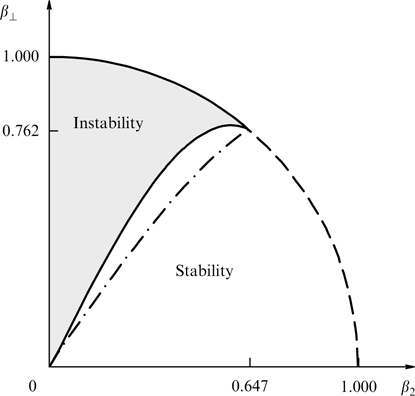
Figure 1. Regions of parameters β2, β⊥ at which plasma with the electron distribution function (36), (44) in the form of a uniformly filled cylinder is subjected or not to Weibel instability with the wave vector parallel to the symmetry axis of the distribution. The dashed curve corresponds to equation  . The ion-to-electron mass ratio mi/me = 1837. For comparison, the dashed-dotted curve shows the boundary of instability for the tubular distribution.
Download figure:
Standard imageThe dispersion curves for γm = 10 and various ratios β⊥/β2 between maximum transverse and longitudinal velocities are plotted in Fig. 2. Specifically, the maximum (relative to  ) increment is achieved for β2 ⪡ 1, γm ⪢ 1 and tends toward
  . It is easy to show that in the relativistic case the range of the wave numbers subjected to instability for the uniformly filled cylindrical distribution under consideration is wider and the growth rates higher than the respective values for the tubular distribution, where the maximum increment amounts to
  .
.
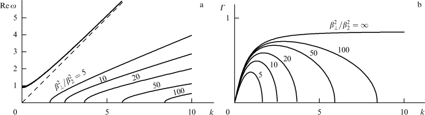
Figure 2. Dispersion curves (39) with substitution of expressions (45) and (46) at γm = 10, mi/me = 1837 and different  values. Frequency Reω and instability increment Γ are normalized to (4πNe2/meγm)1/2, and wave number k = kx is normalized to (1/c)(4πNe2/meγm)1/2. The dashed line corresponds to the straight line ω = ck over which the dispersion curve of the electromagnetic (stable) wave of no interest to us is depicted.
Download figure:
Standard image1.3.4. Estimates of a saturating magnetic field
The nonlinear dynamics of relativistic Weibel instability, unlike the linear ones, elude such strict mathematical analysis. The available occasional numerical studies [40, 51, 52, 56, 60, 87, 96, 144, 150–152] give evidence that instability is saturated as the degree of PDF anisotropy decreases and spatially quasichaotic current structures are formed, part of them having a long-lived magnetic field due to adequate self-consistency with the spatially inhomogeneous anisotropic PDF. This section is confined to the simple qualitative estimation of magnetic fields saturating instability. For certainty, we consider a single sort of particles. Specific features of instability saturation related to the multicomponent plasma composition are discussed in Refs [50, 54, 153].
The linear stage of instability development definitely terminates when the newly formed electromagnetic perturbations markedly alter the momentum distribution of the particles responsible for instability and radically mix their trajectories on the field nonuniformity scale, if harmonics are generated within a wide enough wave number range Δk.
Various estimates of a saturating magnetic field are discussed in Refs [33, 40, 41, 50, 153]. The simplest estimates of the saturation level are obtained on the assumption that the rotation angle of a particle's velocity in the magnetic field Bsat being generated becomes close to unity during the time on the order of the reverse increment time. Then, the cyclotron frequency in the quasi-uniform saturating magnetic field becomes equal to the instability increment Γ:

Substituting the maximum increment in the form of  and taking into consideration that such a growth rate is realized for the wave numbers
  yield
yield
This means that the energy of a magnetic field saturating Weibel type instability can be of the same order of magnitude as the particle kinetic energy in both relativistic and nonrelativistic plasmas at Γ ∼ kυ. If inequalities Γ ⪢ kυ or Γ ⪡ kυ are satisfied for the wave numbers of harmonics growing with an increment on the order of Γ, the saturating (quasiuniform) magnetic field will be weaker and will not reach the 'equipartition' magnitude.
In the difficult-to-realize hypothetical case of Γ ⪢ kυ, saturation takes place when the change in particle momentum over inverse increment time under the effect of the inductive electric field Esat = ΓBsat/kc accompanying the appearance of a magnetic field becomes equal to the characteristic particle momentum mυγ, i.e., eEsat/Γ ∼ mυγ. In this case, the saturating magnetic field is thus independent of the growth rate: Bsat ∼ mcγkυ/e. This estimate of the onset of the nonlinear stage corresponds to 'magnetization' of plasma particles when their gyroradius becomes equal to the scale of growing large-scale perturbation.
In the case of a small exceedance of the Weibel instability threshold (or in the case of weak anisotropy), when Γ ⪡ kυ, a relatively large-scale magnetic field with the wave numbers  is generated and most particles have time to undergo displacements over the distance equaling many harmonic wavelengths of this field in the inverse increment time, as they move in the magnetic field of alternating signs and change their velocity direction much more slowly, on average, than in the magnetic field of constant signs. As a result, the deflection angle for a harmonic in space perturbation is estimated as (eB/mcγΓ)(Γ/kυ); in the case of generation of a large number of independent random harmonics in a wide wave number range Δk ∼ k, the particles' velocity deflection angle varies in accordance with the diffusive transport and reaches a value on the order of
  in the inverse increment time. In the last most realistic case, the energy density of the magnetic field at the time of saturation approaches a value around
if the saturation condition relies on the equality between the characteristic magnetic field scale 1/k and the root-mean-square of the additional particle displacement occurring in the inverse increment time due to diffusive velocity fluctuations on the order of ϕυ.
Both coefficients in parentheses in relation (50) are smaller than unity and define the difference between this estimate and the maximally possible value (49). Naturally, maximum energy density is achieved in magnetic fields with scales around 2π/k corresponding to the maximum increment. These scales are small compared with the gyroradius of free particles. For weak-anisotropy PDFs with Γ ⪡ kυ, the known estimate of energy density in a saturating magnetic field, corresponding to the approximate equality of increment Γ to the bounce-oscillation frequency  of the particles in the vicinity of zero magnetic field regions [5, 33, 50, 150], is likely to underestimate the true value by a factor of kυ/Γ, since, in general, only a small number of particles are subject to bounce-oscillations. Certainly, these estimates of the magnitude of a saturating magnetic field for Weibel instability of this sort of particles and the role of particles trapped by the magnetic field should change under special conditions or geometric restrictions imposed by external influences, the selection of some unstable spatial harmonics or the contribution from other plasma fractions, etc.
In what follows, we consider various current structures formed by the self-consistent motion of both transit particles and those trapped by the magnetic field. The latter are always present in some number, at least in association with certain directions of motion corresponding to bounce-oscillations in the vicinity of the magnetic field minimum. However, the self-consistent current structures under consideration, generally speaking, allow an arbitrary relationship between the particle gyroradius and structure period, including the possibility of situation with rH ⪡ 1/k, when practically all particles become trapped ('magnetized'). Because the saturation of Weibel instability occurs earlier, for krH ≳ 1 (see above), the formation of such current structures with strongly magnetized particles is possible only due to essentially nonlinear plasma dynamics or under the influence of external factors. To recall, of primary importance (see Section 1.2) is the description of a self-consistent magnetic field and current configurations on scales greater than or equal to plasma ones, when charge separation can be disregarded, at least in the absence of external factors.
2. Analytical description of magnetostatic neutral structures in a plasma with arbitrary energy distribution of particles
2.1. Method of invariants of particle motion
The description of stationary configurations of the magnetic field in a collisionless plasma is based on Vlasov's kinetic equations (4) for the distribution functions fα(r, p) of particles over momenta p = γαmαvα of all sorts of particles α and magneto- and electrostatics equations. Certainly, only solutions bounded in the entire space are considered in the absence of boundaries.
Equations div B = 0 and rot E = 0 are satisfied automatically when moving to a description of fields B = rot A, E = −∇φ by vector and scalar potentials, A and φ, the equations for which have the form

Because the phase space of a single particle is hexadimensional, the trajectory of each particle in stationary fields is chosen unambiguously based on a set of five coordinates, bearing in mind that there is such a set of five independent functions ( α1(r, p), α2(r, p), α3(r, p), α4(r, p), α5(r, p)), the values of which are constant along particle trajectories. In the stationary state, the distribution function has a constant value at the phase trajectory of each particle [106, 154] and thus it can be expressed via functions 1, ..., 5: fα(r, p) = fα(α1, α2, α3, α4, α5). In this case, kinetic equation (4) is satisfied automatically for any dependence of fα on α1, ..., α5. Such a substitution of variables is of highest practical interest when several first functions α1(r, p), α2(r, p), ... can be written out analytically, i.e., in the form of explicit integrals of motion, while the remaining ones (α) are unrelated to the distribution function fα [155, 156].
One of the integrals of motion in stationary fields is the particle energy  (its existence is due to the absence of explicit time dependence in all starting equations).
In what follows, we confine ourselves to the analysis of stationary configurations homogeneous along a certain z-axis to preserve for each particle the projection of its generalized momentum onto this axis: α2 ≡ Pz = pz + (eα/c)Az.
If, in addition, a system is uniform along the y-axis, as everywhere below except Section 2.4, the projection of the generalized momentum on this axis: α3 ≡ Py = py + (eα/c)Ay is also an integral of motion (see Sections 2.2 and 2.3).
The integral of motion for a system cylindrically symmetric with respect to the z-axis (pinch-like configuration) is the projection of the generalized momentum onto this axis: α3 ≡ Lz = xpy − ypx + (eα/c)(xAy − yAx). In such a case, it is convenient to use a cylindrical coordinate system. In the case of z-pinch, when the current is parallel to the z-axis and does not depend on z (according to the law of charge conservation), there is actually a single azimuthal component Bφ of the magnetic field, and the problem reduces to an unidimensional magnetostatic equation having very few known exact solutions. Therefore, we only briefly mention the problem of cylindrically symmetric filaments (see Section 2.4), even though it is of importance for cosmic plasma physics, e.g., in the collisionless shock wave theory. In the case of θ-pinch with only the azimuthal current component depending in the general case on z, the magnetic field is essentially two-dimensional and the exact solution of the respective two-dimensional magnetostatic equation is even more difficult to find. There are examples of such a solution for Maxwellian and κ-distributions. It is a self-similar structure defined by the unidimensional equations for a magnetic flux; for the κ-distribution with parameter κ = 7/2, it is described by a simple analytical formula [157]. Such solutions can be helpful for modeling global magnetospheric planetary and stellar structures.
When distribution functions depend only on the integrals of motion, fixation of the shape of these dependences immediately after integration on the right-hand sides of equation (51) turns the integral system into an ordinary set of partial differential equations, with one notable subtlety being that different regions of space may contain particles having identical values of all integrals of motion with mismatched trajectories in the phase space [158–160] (e.g., two particles with equal energies oscillate in the periodic electrostatic potential near two different minima of this potential). The fact that the values of the distribution function at these two trajectories may be different is not in conflict with a stationary kinetic equation. To construct distributions of this type, it is necessary to solve the equations separately in different parts of space and thereafter join the solutions together at the boundary. An example of this procedure for an electrostatic problem is presented in Ref. [161]. We confine ourselves to the construction of solutions with universal dependences fα(α1, ..., α5), identical for all points in space.
Note also that, for certain magnetic field configurations with frequent particle oscillations on the field nonuniformity scale, the particle motion can be described based on additional approximate (quasiadiabatic) invariants. Examples of such quasiadiabatic invariants are well known for trapping configurations, such as the first (magnetic moment-related) and the second (longitudinal) adiabatic invariants [162]. Other examples of importance for describing particle motion in the tail of Earth's magnetosphere are invariants Iz = (2π)−1 ∮ pz dz and Iχ = (2π)−1 ∮ pχ dχ [34, 35, 163, 164]. However, unlike exact invariants, they lead in general only to the integral relation of current and charge densities to vector and scalar potentials, and allow only an approximate description of the contribution from various particle fractions to the self-consistent current sheet. For this reason, they will not be used in the present review, which is confined to exact solutions (an example of the approximate solution for the Harris sheet with a weak external transverse magnetic field is presented in Ref. [165]).
Options for an exact solution of stationary Vlasov–Maxwell equations with nonzero charge density and scalar potential are very limited and were discussed largely in connection with a narrow class of cylindrically symmetric rotating plasma configurations [36, 166] (analogous to the known MHD configurations [79, 167]), in which particles have 'shifted' Maxwellian or κ-distributions. (We are not interested here in the well-known currentless stationary charge density distributions in the plasma [161, 168, 169], the search for which is also based on the method of invariants of particle motion.) As a rule, electrostatic structures with nonzero charge density inside the plasma prove to be unstable, at least on scales much greater than the Debye scale, as a consequence of Debye screening [166, 169, 170]. The presence of quasi-stationary charge separation cannot be ruled out in narrow layers with substantially changed plasma properties, e.g., at the plasma border determined by the external magnetic field or in the region of contact between plasma structures with markedly different parameters, which is stabilized by the magnetic field. Today, however, there are no generally accepted concepts of such current structures and the more so their stability [171]. The authors of Refs [36, 160, 165] took account of nonzero charge density in the presence of an external magnetic field and external forces, e.g., gravity, or other invariants of motion in PDFs, such as angular momentum in cylindrically symmetric current structures.
In what follows, we confine ourselves to neutral current configurations with φ ≈ 0 and ρ ≈ 0. The frames of reference in which this condition is fulfilled are sometimes called De Hoffmann–Teller systems [34, 172, 173]. Certainly, such a condition fulfilled in one frame of reference (being used) is not necessarily satisfied in other inertial frames of reference moving at an angle to the magnetic field. The stationarity of the whole structure remains intact in such frames, as is well known for the Harris sheet with shifted Maxwellian distributions of electrons and ions that contains a nonuniform electric field and charge density correlated with it in frames of reference moving along the current density [174]. The same is true of relativistic self-consistent current structures [30, 175–178], e.g., with Juttner particle distribution, but is not always taken into consideration when estimating the role of electrostatic fields and violation of quasineutrality in analytically sought self-consistent current structures; such an incorrect statement of nonfulfillment of the condition of plasma quasineutrality can be found in Ref. [26].
Because of the difficulty of the magnetostatic problem in question, some of the solutions obtained explicitly or implicitly apply only to part of the particle fractions present in the plasma but allow the inclusion of other fractions or background plasma to ensure fulfillment of some natural conditions, e.g., nonnegativity of the concentrations of all fractions or general electroneutrality of the plasma. For example, the last condition can be satisfied by assuming that currents are produced by electrons alone, solving problem (51) for electrons, and adding the resting positive particles (ions or positrons) with the same spatial density distribution to the final solution. Another way to ensure plasma electroneutrality consists of using charge inversion of the particle distribution function, i.e., by setting f+(p) = f−(−p) = f(p), N+ = N− = N/2 at each point, with '+' and '−' standing for the quantities related to positively and negatively charged particles, respectively.
Certainly, the application of the exact solutions thus obtained describing neutral current configurations to the interpretation of plasma structures in real experiments or numerical calculations implies the possibility of neglecting overall charge density or taking account of disturbed electroneutrality in the solutions being used by any expansion of PDFs modeling the structure of the magnetic fields and currents using equations (51). As regards the nonstationary solutions of the Vlasov–Maxwell equations describing the transition of a nonequilibrium plasma to the magnetostatic configurations of interest and, in particular, the formation of nonlinear Weibel waves or solitons [33, 171], there is no clear analytical picture of the situation due to a number of complicating circumstances, e.g., it is impossible, in general, to satisfy the kinetic equation with the use of PDFs depending only on invariants of particle motion; the equations for the scalar and vector potentials prove to be related, generally speaking, nonlinearly; obtaining physically meaningful solutions requires consideration of external forces and/or certain boundary conditions, etc. These matters are beyond the scope of the discussion below.
2.2. Self-consistent distributions dependent on three invariants of particle motion and current sheets with magnetic field shear
Let all quantities depend only on a single spatial coordinate x, and the magnetic field be perpendicular to the x-axis. Then, it can be described with the use of the vector potential having two components, Ay(x) and Az(x):

The magnetic lines of force of such a field are by necessity straight lines orthogonal to the x-axis, and integrals of particle motion are the total momentum and two components of the generalized momentum:
while any distribution function of the form fα = fα(p, Pz, Py) identically satisfies the kinetic equation [106, 179]. The second equation in system (51) gives the condition of plasma neutrality
In general, current sheets with the shear of the magnetic field (52) are described by two coupled equations
in which current is expressed through the xx component of the tension tensor depending on the components of the vector potential (see, e.g., papers [24, 159]):

with plasma pressure nonuniformity being totally determined by the spatial dependence of the vector potential in accordance with the known balance relation

In the specific case of Maxwellian distribution functions for which the energy dependence is exponential, this component of a tension tensor reduces to the sum of products of concentrations by temperature for the particles of all fractions [156, 173, 180]. Generally, the same profile of the xx component can be provided by different anisotropic distribution functions, and unambiguous restoration of their dependence on generalized momenta Py and Pz through a given profile pxx(x) is impossible, in contrast to the special case of Maxwell distribution functions [3, 7, 13, 159, 181].
It is worthwhile to note that, according to Refs [7, 24, 155, 159, 160, 170, 173, 182], it is possible to take account of weak disturbances of plasma quasineutrality for self-consistent magnetostatic structures described by equation (55) without using the Poisson equation for the electrostatic potential φ, when its presence in the particles' distribution functions by virtue of energy invariant  alters the dependence of the xx component of the tension tensor pxx on the Ay, z components of the vector potential mediated through the φ = φ(Ay, z) bond imposed by the condition ρ ≡ −∂pxx/∂φ ≈ 0. The first attempts to apply this condition in the analytical and numerical searches for self-consistent structures with violated quasineutrality were reported in Refs [155] and [159], respectively, but hopes to obtain physically meaningful analytical solutions in such a form remain unjustified.
The solution of the system of coupled equations (55) is known only for very special cases that can hardly be regarded as representative, including those related to PDFs, particularly taking into account the functional freedom in distributions correlated with fixed configurations of the magnetic field and current (see, e.g., Refs [7, 13]). The first example of such a solution with a shear in the form of a combination of a uniform magnetic field and two sheets having identical Harris current profiles tracing tanh x [2] and orthogonal magnetic fields was found in Ref [3] for 'shifted' Maxwellian distributions of electrons and ions having similar temperatures. In this example, the profile of the current directed along the uniform magnetic field is determined by the Harris current sheet in which distributions of particles of all types contain the same exponential dependence on the vector potential, and the orthogonal current corresponds to the generalized Harris sheet in which particle distributions contain a linear superposition of two exponential dependences on the vector potential differing by a factor of 2 (see Section 3.2.1).
A simpler example discussed in Refs [7, 13, 24] concerns with an elliptical rotation of the magnetic field vector according to the harmonic law with the displacement along the inhomogeneity x-axis for a nonrelativistic plasma with distribution functions whose anisotropic part is the product of the Maxwellian distribution of particles over energy and their generalized momentum squared  . Reference [38] demonstrates that this solution also holds for a relativistic plasma with arbitrary (non-Maxwellian) particle distributions over energy, even different for various sorts of particles. In addition, it is easy to show that the energy density of plasma particles cannot be much lower than that of the magnetic field, while the spatial scale of its changes is not confined by the particles' gyroradii and can be arbitrarily small, provided the concentration of particles is sufficiently high.
The general approach to the construction of such solutions with the shear of the magnetic field for the arbitrary particle distribution over energies is described in Section 2.6. It allows us to obtain current sheets with the magnetic field shear by pairwise combination of any known shearless current sheets, with the distribution functions in each sheet being dependent not only on the energy but also on one of the two orthogonal components of the generalized momentum Py, z. The first report on such neutral configurations appears to be implicitly presented by Kan [173], who used the Maxwellian distribution over energy and superposed the Harris and Nicholson [183] sheets in which particle distributions exponentially depend on the linear and quadratic functions of the generalized momentum, respectively. Strictly speaking, this solution is possible only in the presence of an external magnetic field, along which the flow of particles forming the Harris sheet is directed, and which ensures the finite thickness of the Nicholson plasma sheet generating the diamagnetic current along the magnetic field of the Harris layer, i.e., orthogonal to the external magnetic field. Such local current configurations also existing in the absence of an external magnetic field have been examined, mostly numerically, starting from Refs [8, 173, 182, 184–186], and by later authors for concrete dependences of particle distribution functions on generalized momenta, such as exp and erf, allowing anisotropic modifications of Maxwellian distributions.
There is a broad class of self-consistent current structures for which equations (55) comprise a system of two coupled nonlinear oscillators accounting for a rather complicated, even chaotic, twisting of magnetic field lines during shift along the x-axis (shear). Thus far, this problem has also been explored only numerically; for example, the chaotic character of a magnetic field shear was demonstrated in Ref. [22], as exemplified by distribution functions in the form of quadratic polynomials of two components of the generalized momentum yielding equations of the following form:

where κ and  are constants.
The authors of Refs [20, 24, 25, 176, 181, 187–190] considered flat sheets with a magnetic field shear under the additional condition j × B = 0, i.e., for forceless configurations in which the magnitudes of the xx component of the tension tensor and the magnetic field are constant [see Eqn (57), (58)]. The simplest example is illustrated by sheets with a helical magnetic field [24, 187–189, 191] By = B0 sin (kx), Bz = B0 cos (kx), in which distributions fα can be arbitrary (nonnegative) functions of both relativistic energy (as in the above case of not strictly helical shear) and generalized momentum squared  , different for particles of different kinds.
The only known periodic forceless sheet with an inhomogeneous magnetic field shear is the so-called Jacobi sheet [190] with the spatial dependence of the magnetic field in the form of elliptic functions, consistent with the modified Maxwellian particle distribution containing combinations of cosinusoidal and two different exponential dependences on the generalized particle momenta. It is easy to see again, following paper [38], that this solution is naturally extended to the case of a relativistic plasma with arbitrary particle distributions over energies. In the limiting case of distribution functions containing a single exponential dependence on the generalized particle momentum in addition to the cosinusoidal dependence, the Jacobi sheet reduces to a localized current sheet referred to as the forceless Harris sheet and describes the rotation of the magnetic field through 180° (domain wall type), as shown in Refs [23, 25, 176, 181]. This solution is actually the known Harris sheet with a shearless magnetic field supplemented by a plasma sheet creating the orthogonal component of the magnetic field and maintaining constant total kinetic pressure of the particles and, therefore, of the magnetic field modulus [see relation (58)] (as in any one-dimensional forceless configurations).
It follows from the equality of Lorentz force and pressure force densities (57) that self-consistent sheared structures do not allow the addition of any, even uniform, external magnetic field leaving them nonmodified. When the shear is absent, i.e., there is only a single Cartesian component of the magnetic field, e.g., By, only an external uniform magnetic field directed along the current (along the z-axis) will not introduce distortions into the structure in the case of cylindrical symmetry of the distribution function with respect to this axis, i.e., in the absence of dependence of function fα on invariant Py (see Section 2.4). In the last case, the addition of a uniform magnetic field leads to a shear of the force lines of the general magnetic field, as shown in Ref. [7] for the Harris sheet. Such an application of the external magnetic field in the case of distribution functions depending only on invariants  and Pz does not change as well two-dimensionally inhomogeneous structures with a self-consistent magnetic field lying in the heterogeneity plane.
The nontrivial approach to the construction of self-consistent current sheets with a wide class of distribution functions ensuring transition between plasma regions with a uniform differently oriented magnetic field was proposed by Alpers [3] (see also Refs [14, 159, 173, 176]). The author analyzed monotonic profiles of vector potential components Ay, z(x) and monotonic dependences of electron and ion concentrations on these components for thermal energy distributions with temperature T, allowing for the one-to-one association of these dependences with the distribution functions of the generalized momentum based on the Gauss transform actually appealing to the expansions of the electron and ion distribution functions in terms of Hermitian polynomials. In a specific case, when these expansions are reduced to superpositions of two exponential functions, one of which depends on one and the other on the other components of the generalized momentum, Py and Pz, this association allowed the discovery of a class of distributions correlated with magnetic field rotation through a finite angle in accordance with the laws

where κ, B1, and B2 are constants (an analogous but symmetric current sheet with B1 = −B2 and an additional uniform magnetic field B2 directed along the z-axis is considered in Ref. [7]). At the periphery of one side of the sheet (x → −∞), the magnetic field is directed along the z-axis with currents of electrons and ions in finite concentrations flowing along it in the opposite directions. At the periphery of the other side of the sheet (x → +∞), the magnetic field is directed at an angle to the z-axis (and the y-axis), while electrons and ions in finite concentrations do not create currents. Current sheets with a shear, similar to the last one and, in essence, not requiring the analysis of distributions depending on three invariants of particle motion, are considered in more detail in Section 2.6.
2.3. Grad–Shafranov equation for current sheets with a shearless magnetic field
Let us consider flat sheets without a magnetic field shear, limiting the discussion to the vector potential with a single nonzero component Az(x) (Ay = 0, Bz = 0) but preserving the dependence of the distribution function on three invariants (53): p, py, Pz. It is convenient to choose the vector potential having a single nonzero component Az. Components Ax and Ay in the chosen geometry of the problem can be set equal to zero through a gauge transformation. In this case, currents flow along the z-axis, and the magnetic field is directed along the y-axis (a variant with the direction-variable magnetic field is discussed in Section 2.6).
Then, the Ampère law is expressed as follows:
where the right-hand part does not involve explicitly spatial coordinates and is some function of Az (at a given dependence of functions fα on integrals of motion). Equation (61) is termed the Grad–Shafranov equation [158, 192]; such equations are well known and widely used in MHD (see, for instance, book [167]).
For the neutral current sheets of interest, this equation was analyzed in Refs [3, 7, 14]. It allows any particle distributions over momenta py responsible for the absence of current along the y-axis. These distributions do not influence the structure of the current sheet and in the simplest case can be chosen in the conventional form of a shifted Maxwellian distribution [17] or even in the form of δ-functions [193–195], which simplifies the interpretation of observational data, e.g., on the current sheet in the tails of Earth's and Jupiter's magnetospheres. In this context, it is worthwhile to mention the implicit solution of the Grad–Shafranov equation [14, 17] that is actually a combination of the known Harris [2] and Channell [7] solutions, i.e., described by a modified Maxwellian distribution containing quadratic dependence on Pz.
Because the magnetic field is directed along the y-axis, the projection of the particle momentum onto this axis is not changed under the effect of the magnetic field, which, in turn, remains unaltered against the particle motion along the y-axis. It is formally reflected in that the projection py enters equation (61) only via the relativistic factor γα. Indeed, the distribution function can be regarded as a set of 'sheets' with different fixed py values that do not intermix. The current density is determined by the total contribution from all such sheets, which allows the Grad–Shafranov equation to be rewritten more exactly taking into account that  is also invariant if p and py are conserved, fα can be represented without loss of generality as functions of pt, pz + eαAz/c and py, and then it is possible to move to cylindrical coordinates py, pt, φ, so that pz = pt cos φ, px = pt sin φ:
Denoting the result of internal integration over py by
yields the transformed Grad–Shafranov equation
The possibility of hitting on analytical solutions to this equation is related in one way or another to a certain fixation of the dependence of function Fα on its arguments and remains poorly known for any general case. In this context, it is worthwhile to mention several attempts at the numerical solution of this problem, e.g., by using expansions of distribution functions in terms of Hermitian polynomials [14, 159, 182] and the possibility of moving to the solution of a simplified problem by practical exclusion of the dependence on one of the two components of the generalized momentum [6, 7, 25, 176–178, 194, 196] (see below).
It should be noted that PDFs arising from self-consistent solutions of equations of the Grad–Shafranov type can be highly varied, e.g., non-Maxwellian in terms of energy and asymmetric or double-humped in terms of coordinates; their realization in nature and experiment is limited only by the requirement of sufficient stability of current sheets, which has thus far been investigated in fragmentary studies (mostly numerically) for a narrow class of perturbations and only for a few examples of current sheets both with and without the magnetic field shear (see, e.g., Refs [8, 38, 175, 197–205]).
2.4. Two-dimensionally inhomogeneous magnetic structures and current filaments with cylindrically symmetric particle distributions
Abandoning the requirement for problem homogeneity along the y-axis makes necessary only the first two of the three invariants of motion (53). The choice of fα in the form of a cylindrically symmetric function depending on these two invariants, namely

gives the Grad–Shafranov equation in the form
This time, it is convenient to move to spherical coordinates p, θ, φ (pz = p cos θ, px = p sin θ cos φ, and py = p sin θ sin φ) and perform trivial integration over the azimuthal angle φ, and to move from integration over the polar angle θ to integration over the momentum projection pz:
The right-hand side of expression (64) or (67) is a function of Az, which is frequently convenient to represent for the qualitative analysis of solutions of the equation in the form −dU(Az)/dAz, expressing it through another function, U(Az), called the Grad–Shafranov potential. Then, one-dimensional equation (64) takes the form of the nonlinear oscillator equation well known from classical mechanics:
while two-dimensional equation (67) is expressed in the form

Notice that the potential U(Az) has the dimension of energy density; it is easy to show that it differs from the component pxx (equal to pyy) of the tension tensor only in the coefficient, as in the one-dimensional case (55), (56), when the cylindrical symmetry of distribution functions was not mandatory and they could depend on three invariants of particle motion.
For certain types of dependence of functions Fα and fα on their arguments, integrals on the right-hand sides of expressions (64) and (67) can be taken analytically, thereby reducing the problem to an ordinary second-order differential equation in the one-dimensional case, and to a partial differential equation in the two-dimensional case. Concrete examples will be considered below.
To begin with, let us touch a cylindrically symmetric case in which the current flows along the z-axis, and Az depends only on the radial coordinate  , but not on the azimuthal angle. In this case, the Grad–Shafranov equation (69) has the form
The analog of this equation in classical mechanics is the equation of motion of a particle in the potential U(Az) in the presence of viscous, i.e., proportional to velocity, friction. The role of time is played by radius ρ, and the role of velocity by quantity dAz/dρ. The coefficient of friction depends on 'time' ρ and is proportional to ρ−1. The boundary conditions also change in comparison with the one-dimensional planar layered case. Coordinate ρ varies within the semiaxis from zero to infinity, and the magnetic field at point ρ = 0 vanishes, i.e., dAz/dρ|ρ = 0 = 0 (otherwise, an infinitely high current density would exist along the z-axis ar ρ = 0 in accordance with the formula for the azimuthal magnetic field Bφ = 2I/cρ, where I is the total current inside a cylinder with radius ρ). In the 'mechanical' analogy, this means that the particle begins to move at ρ = 0 without an initial speed. In fact, only three qualitatively different options are conceivable.
I. The region of values of the vector potential component Az is restricted; as ρ grows, the value of Az infinitely oscillates near the bottom of the potential well. In the case of general position, the shape of the well can be approximated by a parabolic profile following the decrease in the amplitude of these oscillations; then, the form of the solution becomes reminiscent of the Bessel function. Amplitudes of oscillations Az of a magnetic field, and those of the current density decrease with increasing ρ as 1/ρ. If the expansion of the Grad–Shafranov potential into a Taylor series near the bottom of the potential well starts from a term other than the quadratic one, the infinite oscillations also appear but their period increases with ρ. The resulting current configuration comprises, formally speaking, an infinite set of concentric current cylinders, of which the outer ones have, as a rule, a higher overall current and lower current density than the inner ones.
II. The region of values of the vector potential component Az is restricted, and its derivative with respect to variable ρ (the azimuthal component of a magnetic field) changes the sign a finite number of times. In this case, the 'motion' of Az begins at ρ = 0 from rolling down the slope of the potential well and ends at the local maximum.1 A few reflections from the walls of the potential well higher than the final peak may occur between the beginning and end of motion. The total current is zero, and the magnetic field decreases with growing ρ faster than 1/ρ. In the case of general position, the peak at the potential profile has the quadratic form, which means that the magnetic field and current density decrease exponentially with growing ρ.
III. The value of the vector potential component Az varies infinitely, which necessarily means that Az changes monotonically and the azimuthal component of the magnetic field has the same sign at all ρ. The current density may be an alternating-sign quantity; however, the current flowing through any round plot perpendicular to the z-axis with the center at this axis has only one sign. The total current can be either finite or zero-valued. A case is possible in which the plasma localized near the z-axis has a density exponentially tending toward zero with distance from this axis.
The first example covers the analytical generalization of the known Bennett pinch to the case of arbitrary energy distributions, which corresponds to the exponential dependence of PDFs on the generalized momentum: fα = Fα0(p) exp (ζαPz/mαc). In this case, the Grad–Shafranov equation takes the form
where A0 = mαc2/ζαeα (assuming this quantity to be the same for all kinds of current-carrying particles α), while W0 is positive and expressed as an integral including an arbitrary function Fα0(p). The family of solutions satisfying the boundary condition dAz/dρ|ρ → 0 = 0 is described by the formula (cf. Refs [1, 179])

and is parametrized by a positive quantity κ, the inverse of the filament radius. If, for definiteness, A0 > 0, κ is positive, too. The corresponding magnetic field
unrelated to the energy distribution of particles, Fα0, is maximum at ρ = κ−1, and amounts to 2κA0. The current density is given by the expression (Fig. 3)
its simple integration gives a total current value of 2cA0 independent of κ and, therefore, of the filament radius.
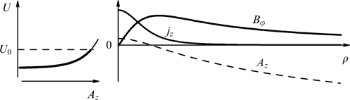
Figure 3. Typical profile of the potential of the Grad–Shafranov equation (71) and the dependences of Az, Bφ, and jz on the cylindrical coordinate ρ for the solutions given by formulas (72)–(74) in the form of the Bennett pinch. Hereinafter, the bold line in the Grad–Shafranov potential plots indicates the region of varying Az values.
Download figure:
Standard imageOwing to the exponential dependence of the PDF on the projection of the generalized momentum, distributions of any kind of particles over momentum at all points of space are similar and differ only in the momentum-independent factor. Therefore, the shape of the particle concentration profile coincides with that of the current density profile: Nα = Nα max/(1 + κ2ρ2)2. The integral of Nα over plane xy gives the number of particles per unit pinch length and is equal to πκ−2Nα max, which once again confirms the possibility of conventionally regarding quantity κ−1 as the radius of the current filament being considered. This radius can be either longer or shorter than the particles' characteristic gyroradius depending on their energy distribution.
Another interesting example is given by the quadratic dependence of the distribution functions on the generalized momentum,  , leading to the linear Grad–Shafranov equation
i.e., the zero-order Bessel equation having under the given boundary condition the following general solution:
Here, unlike the preceding example, the free parameter is amplitude Az max, and the spatial scale k−1 is determined by the energy distribution of particles. The shape of the current density profile coincides with that of the vector potential profile, because jz ∝ dU/dAz and  , while the magnetic field profile is described by an order-one Bessel function of the first kind: Bφ = −kz max J1(kρ). The profiles are plotted in Fig. 4 where, as in Fig. 3 and other figures presenting Grad–Shafranov potential plots, the bold line indicates the region of varying Az values.
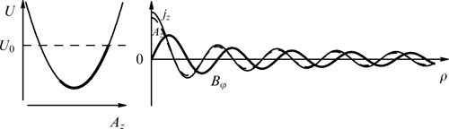
Figure 4. Quadratic profile of the Grad–Shafranov potential and the dependences of Az, Bφ, and jz on the cylindrical coordinate ρ for the Bessel type solution (76).
Download figure:
Standard imageThis solution oscillates with the growth of the radial coordinate ρ, while the amplitude of magnetic field oscillations decreases in proportion to ρ−1/2, and the amplitude of current oscillations inside a cylinder of radius ρ increases proportionally to ρ1/2. The amplitudes of magnetic field and current density oscillations decrease with distance from the axis, when kρ ⪢ 1, while solution (76) is increasingly less different locally from the harmonic one. Therefore, upon exceedance of a certain radius ρf at which the characteristic gyroradius rH of particles becomes on the order of the inhomogeneity scale k−1, the energy density of the magnetic field becomes by necessity lower than equipartition one, the degree of distribution function anisotropy is close to a constant of order 2, and Weibel type instability can be expected to develop in this region. Of the greatest interest in this context is the internal part of solution (76) (ρ ≲ ρf), where rHk ≲ 1, and in the absence of a large fraction  of isotropic particles the energy density of the magnetic field can be on the order of the equipartition one.
Other interesting classes of solutions emerge when using distribution functions of particles with a higher order of polynomial expansion in terms of the generalized momentum Pz. Then, the Grad–Shafranov potential as a function of the vector potential component Az is a polynomial of the same order, and the spatial structure of the fragment can be rather complicated. For example, if the range of Az variations is bounded and Az monotonically, without oscillations, tends toward a certain constant, while ρ tends to infinity, the filament it describes is the central current surrounded by an equal and opposite current, such that the total current is zero (with more than one change in the current density sign being possible). Figure 5a presents an example of the solution of such a form for the Grad–Shafranov equation with the potential proportional to  at a certain constant A0 value. This solution corresponds to such a set of PDF parameters at which the representative point of Az as a variable of equation (70) tends to a local maximum in the Grad–Shafranov potential as ρ → ∞. In this case, the only nonzero magnetic field component Bφ has one sign everywhere, and the current density changes the sign only once as the coordinate ρ grows.
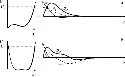
Figure 5. Profile of the Grad–Shafranov potential U(Az) and the dependences of Az, Bφ, and jz on the cylindrical coordinate ρ for (a) a filament with the countercurrent,  , and (b) a filament with the change of direction of the azimuthal magnetic field,
  .
.
Download figure:
Standard imageIf the Grad–Shafranov potential takes the form of a fourth-order polynomial, e.g.,  with a certain constant A0, the solutions become possible with more than one change of current density direction and a few changes of the component Bφ sign. The solution with Bφ changing the sign only once and the current density being two cylindrical countercurrents embedded within each other is presented in Fig. 5b. The analysis of the asymptotic behavior of filaments of this type at large ρ reveals their exponential decrease.
One more important class of current filaments is represented by solutions of the Grad–Shafranov equation for distribution functions in the form of the sum of two components that exhibit exponential dependence on the generalized momentum Pz with different exponents whose ratio equals w and may have arbitrary dependences on particle energy:

Here, as in the case of the generalized Bennett pinch, A0 = mαc2/ζαeα, and constants W1 and W2 are given by integrals of energy distributions. The most interesting case is that of exponents having identical signs, which allows us to consider A0 and w, for certainty, as being positive. Moreover, it can be assumed, without a loss of generality, that w < 1, and one of the two exponents (second) changes faster than the other.
If W1 > 0 and W2 > 0, while w ⪡ 1, a double-scale solution is possible, as exemplified for w = 0.1 in Fig. 6a. If W1 > 0, W2 < 0, the solution will take the shape of a 'tubular' current filament in which a current density maximum is shifted from the cylindrical symmetry axis to a certain cylinder around it (Fig. 6b).
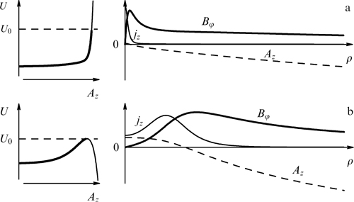
Figure 6. Profile of the Grad–Shafranov potential U(Az) and the dependences of Az, Bφ, and jz on the cylindrical coordinate ρ for (a) the double-scale filament, U(Az) ∝ exp (Az/A0) + exp (10Az/A0), and (b) the 'tubular' filament, U(Az) ∝ exp (Az) − exp (2Az).
Download figure:
Standard imageThe total current in these two solutions differs from 2cA0 obtained upon direct generalization of the Bennett pinch, which accounts for the different asymptotic behavior of solutions far from the axis, despite the fact that only one of the two components on the right-hand side of Eqn (77) is essential at large ρ, and the form of the equation coincides with that of equation (71) having solutions in the form of Bennett type pinches. The analysis of the asymptotic behavior of such fragments at large ρ shows that the magnetic field decreases in inverse proportion to the distance from the axis.
Let us consider in brief solutions to the two-dimensional Grad–Shafranov equation, irreducible to planar layered or cylindrically symmetric ones for the two simplest cases, viz. quadratic and exponential forms of the Grad–Shafranov potential. See Refs [11, 31, 32, 49, 157, 206, 207] for other possible solutions of the two-dimensional Grad–Shafranov equation.
The evident solution for the quadratic Az-dependence of the Grad–Shafranov potential, considered above in the analysis of the filament with the Bessel profile, in the two-dimensional case (69) is the arbitrary linear combination of harmonics:

with arbitrary phases ϕl and angles φl. Despite the identical wave number k of all harmonics [see Eqn (76)], the resultant current and magnetic field structures can be complicated and even quasichaotic in space.
It is easy to show that the magnetic field energy for any set of harmonics (78) can be close to 2/3 of the particle kinetic energy in a nonrelativistic plasma, and 1/3 of the total particle energy in a relativistic plasma, because interference terms from the items with different directions of vector k vanish upon averaging over space. Moreover, in the case of a magnetic field of equipartition order, the gyroradius of typical, not highly energetic particles is almost everywhere smaller than or nearly the same as the characteristic spatial scale k−1 of a self-consistent current structure [208].
The special choice of amplitudes, phases, and directions of sinusoidal field components Al = A1 = const, ϕl = 0, φl = πl/n yields the solution
approximating the cylindrically symmetric solution (76) (Fig. 7a) not far from the axis. At n = 2, the directions of the currents in the regular grid of current filaments are distributed in a chessboard pattern, and the current density vanishes at the square borders, as shown on the left panel of Fig. 7b. At n = 3, the unidirectional current filaments make up a hexagonal grid with the countercurrent distributed between them (right panel, Fig. 7b).
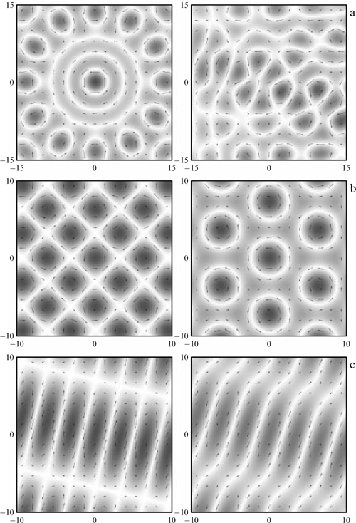
Figure 7. Two-dimensionally inhomogeneous current configurations. The shades of gray characterize the current density modulus (white color denotes zero density), and arrows indicate magnetic field magnitude and direction. The scale on each axis is counted in k−1 units. (a) Configurations described by potential (78) with n = 6 sinusoidal components: left panel corresponds to the special choice of directions, amplitudes, and phases (79), and right panel to their arbitrary choice. (b) Configurations described by potential (79) with n = 2 (left) and n = 3 (right) sinusoidal components. (c) Configurations described by potential (78) with n = 2 sinusoidal components with angle φ2 − φ1 = 30° between them: A1 = A2 (left), and A1 = 2A2 (right).
Download figure:
Standard imageGiven the single term in sum (78), there is a purely harmonic one-dimensional nonlinear solution, i.e., periodically alternating oppositely directed current sheets. Summation of two terms with similar angles φ and amplitudes yields a grid of alternating current sheets of bounded length, while summation of two terms with similar angles φ and markedly different amplitudes results in periodically modulated current sheets. Figure 7c illustrates the case of φ2 − φ1 = 30°.
It is easy to check that in all the above cases the solution in the form (78) for any distribution function  is not subject to Weibel instability for short-wave perturbations with scales smaller than k−1 in the regions of strongest anisotropy of particle distributions. Indeed, the quantity Az in such regions is close to zero, the degree of anisotropy is of order 2, and [according to criterion (27)] wave numbers of unstable perturbations are limited in accuracy by k [cf. formulas (26) and (76)].2
Finally, for the distribution function showing an exponential dependence on the generalized momentum component Pz and containing an arbitrary factor depending on particle energy, two-dimensional solutions of the Grad–Shafranov equation
can be obtained by analogy with the cylindrically symmetric case of the Bennett pinch (71) in the form generalizing the Fadeev solution [209]:
Here, the free parameter μ is responsible for the degree of structural inhomogeneity along the y-coordinate. At μ = 0, we obtain generalization of the Harris sheet for the case of arbitrary energy distribution of particles, which is discussed in detail in Section 3.2.1. Another free parameter κ−1 assigns the scale of magnetic field changes on the x- and y-axes. The equality of these parameters is essential.
The current density in solution (81) is given by the formula
indicating that a self-consistent current structure at large enough μ actually consists of a chain of generalized Bennett pinches arranged with a period of 2π/κ and carrying 2cA0 current each. The magnetic field and current density entering solution (81) at two different values of the imhomogeneity parameter μ are shown in Fig. 8.

Figure 8. Two-dimensionally inhomogeneous configurations described by potential (81) at different values of the inhomogeneity parameter μ. The shades of gray show current density (white color denotes zero density), and arrows indicate magnetic field strength and direction. The scale on each axis is counted in κ−1 units.
Download figure:
Standard imageFrom the fact that available two-dimensional analytical solutions describing self-consistent current structures in collionless plasma are very fragmentary, exhibit at odd times singularities, and do not provide the overall picture of possible self-consistent current structures we will not discuss them anymore (see, e.g., Refs [5, 6, 10, 32, 49, 157]). Therefore, we will focus below on a diversity of one-dimensional configurations for which the modern concepts seem to be much more complete.
2.5. Classification of planar layered magnetostatic structures with a shearless magnetic field
In 'one-dimensional' geometry and in the absence of a dependence on y- and z-coordinates in the class of distribution functions depending on three integrals of motion, current sheets are described by the Grad–Shafranov equation (68) with potential U(Az) equaling the integral over Az on the right-hand side of equation (61). For the qualitative analysis of solutions, it is convenient to turn to an analogy with the equations of motion of a material point in the coordinate-dependent potential known from classical mechanics. The role of the material point coordinate is played by the vector potential component Az, the role of time by the spatial variable x, and the role of velocity by the magnetic field −By = dAz/dx taken with the opposite sign. The first integral of equation (68), viz.
is of special importance, since it allows us to write out the implicit representation of the solution by the designated constant U0 and the chosen position (point x0):
Let us consider which classes of current structures are possible depending on the potential shape U(Az) and U0 value. From very general considerations, three qualitatively different situations can be distinguished: namely, magnetic field By with x varying from −∞ to +∞ can change sign several times, change it but once, or not change it at all. It gives the following classification.
I. It is evident from the analogy with a mechanical system that a self-consistent current structure is periodic if the magnetic field changes sign more than once. In this case, function U(Az) serves as a 'potential well' and curve Az(x) reflects oscillations (generally speaking nonlinear) in this well between some two extreme values Amin and Amax, such that U(Amin) = U(Amax) = U0. The magnetic field vanishes at the turning points corresponding to Az = Amin and Az = Amax (and only at these points), while the profiles of the magnetic fields with opposite signs between these points are mirror images of each other: if By(x0) = 0, then By(x) = −By(2x0 − x). Accordingly, current density proportional to the derivative of magnetic field By with respect to x is symmetric relative to any plane of a zero magnetic field.
II. Let us turn to the magnetic field changing sign only once. A plane in which the magnetic field vanishes can be taken (without the loss of generality) as the origin of the x-coordinate, By(x = 0) = 0. Then, the dynamics of function Az(x) in the vicinity of x = 0 corresponds to reflection from the potential barrier U(Az). The magnetic field is antisymmetric, By(x) = −By(−x), and current density symmetric jz(x) = jz(−x). Current density, unlike the magnetic field, can be a fixed-sign quantity and change the sign any even number of times, provided the potential profile U(Az) is nonmonotonic but contains irregularities that do not, however, ascend above U0 = U(Az(x = 0)) in the entire region of Az variations. Because the derivative of function Az(x) changes sign only once, there is a passage to the limit: limx→−∞ Az(x) = limx→+∞ Az(x) that can be either finite or infinite.
If the limit is finite, limx→∞ Az(x) = A0, U(A0) = U0 and dU(Az)/dAz|Az = A0 = 0, whence it follows that the 'motion' of point Az actually consists of rolling down a hilltop3 at Az = A0, reflection from the turning point at x = 0, and climbing back uphill to point Az = A0. In the case of general position, the potential in the vicinity of Az = A0 is approximated by a parabola, and functions Az(x) − A0, By(x), and jz(x) as x → ±∞ exponentially tend toward zero.
If the limit is infinite, limx→∞ Az(x) = ±∞, the value of potential U(Az) over the entire ray from Az(x = 0) to Az(∞) corresponding to infinity does not amount to higher than U0. In this case, the magnetic field far from the point x = 0 cannot be exponentially small. It can either decrease in the power-law fashion no faster than 1/|x| or tend toward a certain nonzero value. (It is assumed here that U(Az → ±∞) = const, because other variants appear to be nonphysical and suggest either indefinitely high magnitudes of distribution functions or the presence in them of essential dependences on infinitely large generalized momenta.) In the case of a field decrease, current density also tends toward zero no faster than 1/|x|2 with a possible change of sign, in contrast to the magnetic field. If the magnetic field tends toward a nonzero constant, the current density can be localized with any power index or even exponentially, with the total current of the entire current structure remaining nonzero.
III. Let the magnetic field not change sign, which means that U(Az) varies monotonically. In self-consistent structures with a magnetic field created and maintained by the plasma itself, it cannot have different magnitudes of one sign far from the current structure. In other words, if the magnetic field does not change sign, then B(x → −∞) = B(x → +∞) = 0 and the current density changes sign at least once, while the total current of the current structure is zero. If the range of Az changes is bounded, the 'motion' of point Az actually consists of rolling down a hilltop of height U0 and climbing up another hill of the same height U0.
In the case of general position, the potential in the vicinity of both tops is approximated by parabolas; therefore, the magnetic field By(x) and current density jz(x) as x → ±∞ exponentially tend to vanish. If the range of Az change is not bounded and Az tends toward the respective infinity, the potential U(Az) tends to U0 and thereby causes a reduction in the magnetic field, while the current structure is asymmetric, with current density exponentially decreasing to one side and decreasing in a power-law manner not faster than 1/|x|2 to the other side. One can imagine a profile of Az such that the region of its changes will be unbounded on both sides [e.g., in the U(Az) ∝ −cosh−2 (Az/A0)) potential], but the shape of the potential needed in this case cannot be obtained analytically using the expansions [e.g., like (173)] with a finite number of terms, considered in Section 3.
When the magnetic field does not change sign, the Grad–Shafranov equation can be used to describe nonself-consistent current structures located in the external magnetic field. In this case, as x → ±∞, the magnetic field tends toward two, generally speaking, different constants, with at least one of them being nonzero, and at least one of the limits, U(Az → −∞) or U(Az → +∞), finite and smaller than U0. If U(Az) is everywhere smaller than U0, while limits U(Az → −∞) and U(Az → +∞) are equal, it suggests an existence of a current structure localized in the external uniform magnetic field, having zero total current. If U(Az) is everywhere smaller than U0 and the above limits are not equal, then the current structure has nonzero total current, while the magnetic field is partly screened by this current [in the case of U(Az → ±∞) = U0, the screening is complete but localization weak—current density decreases no faster than 1/|x|2). After U(Az) reaches the U0 value at a finite magnitude of the vector potential component Az, the derivative of potential U(Az) at this point equals zero by virtue of the above assumption of the fixed-sign magnetic field, and we concern with complete screening of the external magnetic field, which enables us to describe the boundary between an nonmagnetized (generally speaking anisotropic) plasma and a plasma (or vacuum) with a uniform magnetic field (see Sections 3.4 and 4.3). In the case of general position, the second derivative of potential U(Az) at the stop point is other than zero, while the magnetic field and current density exponentially decay as they go deep into the plasma.
2.6. Superposition of current sheets with orthogonal magnetic fields
The above classification of current sheets can be extended to the sheared magnetic field for PDFs representable as the sum of two cylindrically symmetric functions with orthogonal axes:

In this simple but yet poorly explored situation, the equations of magnetostatics break down into two Grad–Shafranov equations
independent of each other but nonlinear in themselves.
Thus, provided two one-dimensional self-consistent solutions to the magnetostatic problem in a collisionless plasma with the cylindrically symmetric distribution functions  and
and  are known, their superposition (85), taken so that the magnetic field of one solution is directed along the cylindrical symmetry axis of the distribution function of the other solution, is also the solution of the same system of equations and satisfies the general equation of pressure balance (58). It allows us to construct solutions with an arbitrary sheared magnetic field, i.e., with the dependence of the rotation angle of the magnetic field in the yz plane on the x-coordinate. The resultant solutions for B = B(1) + B(2) are readily classified from the shape of the respective Grad–Shafranov potentials U(1)(Az) and U(2)(Ay), as described above.
To recall, the periodic helical structures or localized current sheets are made possible with the unchangeable direction of magnetic field rotation, as well as sheets undergoing single changes in the shear direction. Each of the two 'combinable' solutions allows the presence of an external magnetic field in agreement with what was said at the end of Section 2.5. Also allowed is the trivial possibility of putting  , where Bz = const, which means the imposition of an arbitrary constant magnetic field By directed parallel to the z-axis, i.e., along the direction of current density, on a flat sheet with a single magnetic field component By. A specific solution of this kind, in which the known Harris sheet is supplemented by one more magnetic field component so that the modulus of the magnetic field is constant in the entire space, was proposed in paper [23].
There are a few less trivial examples of superpositional current sheets with a sheared magnetic field, the number of which can be substantially increased using the aforementioned analytical method for the construction of such solutions. For example, solution (60) obtained in Ref. [3] and a superposition of Harris and Nicholson sheets [173] discussed in Section 2.2 can be easily generalized to the case of particle distribution functions containing factors with an arbitrary dependence on the particle energy. Reference [7] reports a wave-like solution in which the distribution function is represented as the sum of two terms, one quadratically dependent on Py, and the other on Pz, with identical coefficients and magnetic fields B(1) and B(2) harmonically depending on the x-coordinate with a similar spatial period. The authors of Ref [25] made use of the exponential dependence of the distribution function on one component of the generalized momentum, and the harmonic dependence on the other, which corresponds for a nonperiodic solution to B(1) ∝ tanh (x/L), and B(2) ∝ cosh−1 (x/L), where L is the characteristic sheet thickness. At a certain relation between these two components, the magnitude of the total magnetic field is constant over the entire space.
Let us turn to concrete examples of self-consistent current sheets with the shearless magnetic field, qualitatively described in Section 2.5 based on special PDF expansions.
3. Typical strictly solvable problems for self-consistent current sheets
3.1. Power-law particle distributions
3.1.1. General power-like form of the Grad–Shafranov potential
Let cylindrically symmetric distribution functions fα in Grad–Shafranov equation (61) be expanded at each momentum p value into the Taylor series over the projection pz + eαAz/c of the generalized momentum containing the vector potential component Az:
It is then easy to take the integral over pz in the expression for the Grad–Shafranov potential [see equation (68)]:
If only a finite number of terms with powers up to d differ from zero in expansion (88), i.e.,  for i > d, the potential U(Az) (89) is the dth degree polynomial, and the removal of the parentheses reveals zero coefficients of
  in formula (89). Only coefficients of this universal polynomial depend on the form of the
  function, i.e., the energy distribution of particles.
It should be noted that formula (89) holds not only at nonnegative integer i, but also at all i ≠ −1, −2, −3, which allows us to consider distribution functions with power-like dependences on the projection of the generalized momentum with negative or noninteger exponents. At i = −1, −2, −3, the expression for the Grad–Shafranov potential is equally well defined and can be obtained from formula (89) by means of the limit passage i → −1, −2, −3, respectively.
It can be concluded that, for cylindrically symmetric distribution functions expanded in powers of the generalized momentum projection, in the case of a finite number of nonnegative powers there is a universal polynomial form of the Grad–Shafranov potential, while energy distributions of particles determine only the finite set of polynomial coefficients. Modeling of the Grad–Shafranov potential profiles in accordance with formula (89) makes possible the analysis of various self-consistent current sheets.
3.1.2. Periodic current structures
To construct the simplest periodic solution, suffice it to be confined to the quadratic term in the polynomial expansion of the cylindrically symmetric distribution function (88):
In this case, the Grad–Shafranov potential (89) equals
and the particle concentration profile is dictated by the dependence of the vector potential on the x-coordinate in accordance with the formula
The term linear in Az can be eliminated from expression (91) by gauge transformation Az ⇒ Az + const, and Az-independent items do not contribute to the Grad–Shafranov equation, since it contains only the derivative dU(Az)/dAz. Therefore, it can be assumed that  .4 Then, the initial nonlinear magnetostatic problem reduces to the linear Grad–Shafranov equation in the form

where the wave number k has already been defined in formula (76). Its solutions in the one-dimensional case are sinusoids

with the arbitrary amplitude Amax and phase φ.
For such solutions with weak enough magnetic fields when variations of the vector potential (therefore, distribution function anisotropy) in a self-consistent current structure are insignificant, there is every reason to expect the emergence of long-wave Weibel instability with scales greater than k−1, but smaller than the characteristic gyroradius rH. The point at issue is perturbations for which a static magnetic field does not play any special role, i.e., dispersion relation (22) gives an increment much bigger than the characteristic gyrofrequency of particles. It follows from the above and the discussion in Section 2.4 that suppression of Weibel instability for solutions (90), (94) should be evidenced only for a strong enough magnetic field, say of an equipartition order, when rH ≲ k−1.
For harmonic solution (94) with quadratic particle distribution functions (90), it is easy to deduce the relationship between the mean magnetic field energy density and mean energy density of particles. For maximally excluded isotropic constituents of the distribution functions,  , we arrive at
For this expression, it is possible to obtain a simple upper bound:
In the relativistic case with Amax much greater than characteristic pc/eα values, B can be close to 1/3.
In the nonrelativistic case, of special interest is the relationship between mean energy density of the magnetic field and mean kinetic energy of particles:
The upper bound analogous to formula (96) for the nonrelativistic case takes the form  , with the values of
  close to 2/3 being attainable at the amplitudes Amax much higher than characteristic pc/eα values. The presence of the nonzero isotropic plasma component described by the distribution function component
  merely decreases the fraction of the magnetic field energy.
Retention of higher terms in polynomial expansion (88) leads to obtaining strongly anharmonic periodic current sheets, as exemplified in Fig. 9 for the case when the U(Az) potential well is symmetric and expansion (88) begins from a high power. It can be seen that at high powers, the potential well almost has a flat bottom and low current density in a large area of space, while the magnetic field is close to constant. In fact, there is a series of alternating current sheets carrying oppositely directed currents separated by portions of currentless plasma with a magnetic field.

Figure 9. Profiles of the anharmonic Grad–Shafranov potential U and coordinate dependences of Az, By, and jz: (a)  , and (b)
  .
.
Download figure:
Standard imageRetention of terms up to the third order inclusive in the polynomial expansion (88) (see details of an analysis of the screened current sheet below) results in an asymmetric potential well and magnetic field profile. Solutions for two different values of the first integral U0 are shown in Fig. 10. The higher the U0 value, the more the solution deviates from a harmonic one. When U0 is close to the local maximum of the Grad–Shafranov potential, the solution becomes a series of screened current sheets (see Section 3.1.3 below for details) arranged periodically in space.

Figure 10. Typical profile of the anharmonic Grad–Shafranov potential (89) in the form of a cubic parabola and coordinate dependences of Az, By, and jz for the periodic solution at two different values of the first integral U0.
Download figure:
Standard imageFinally, retention of terms up to the fourth order inclusive in polynomial expansion (88) (see the analysis of the double current sheet below) yields even more intricately shaped profiles, exemplified in Fig. 11. Examples of anharmonic periodic solutions based on exponential expansions of the distribution function, for which the magnetic field and current profiles are described by analytical formulas, are presented in Section 3.2.2.
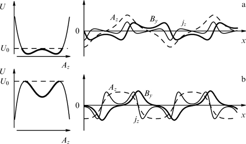
Figure 11. Variants of the profile of the Grad–Shafranov potential (89) in the form of a bi-quadratic parabola and coordinate dependences of Az, By, and jz for periodic solutions.
Download figure:
Standard image3.1.3. The screened current sheet
Let us consider a localized solution in which the magnetic field vanishes at infinity, retaining items up to the cubic one in expression (88):
After elimination of the Az-independent terms making no contribution to the equation, the Grad–Shafranov potential (89) has the form
We are interested in the localized solution in which the value of the vector potential component Az as x → ±∞ tends toward constant, the same at both infinities. Taking account of the gauge transformation, it can be assumed without the loss of generality that this constant equals zero, i.e., the local maximum of potential (99) is reached at the point Az = 0, which suggests the absence of items linear in Az:
Then, the solution of the Grad–Shafranov equation (68) under the boundary conditions Az(x → ±∞) = 0 is found analytically:
Hence follows the magnetic field
current density
and concentration
The final expression for the particle concentration as a function of the x-coordinate is obtained by substituting solution (101) into formula (104), and has a rather cumbersome form.
Both the magnetic field and current density reach the following maximum magnitudes:
To recall, it was assumed in the foregoing that the condition
responsible for the presence of a local maximum (but not minimum) of the Grad–Shafranov potential at point Az = 0 is fulfilled. Violation of this condition does not interfere with the solution in the form of the screened current sheet by virtue of the cubic potential profile; if it has a local minimum at Az = 0, then the local maximum occurs in another place. However, this solution does not satisfy the condition Az → 0 as x → ±∞, and is described by different formulas.
The characteristic thickness of the current sheet is found from expressions (101)–(103) as
and can be compared with the gyroradius of particles having a certain momentum p0 in the magnetic field maximum:
The ratio of the gyroradius to the characteristic sheet thickness is given by
For particles forming the current sheet of interest, this ratio can be either much smaller than unity (magnetized particles) or much higher than unity (most particles pass through the current sheet hardly deflecting in its magnetic field). The shapes of the vector potential, current density, and magnetic field profiles are similar in all cases, as shown in Fig. 12a. The particle concentration profile can have either a single maximum in the center or three maxima, one central and two lateral, depending on ratio (108). The central current sheet is completely screened by two lateral ones, so that the magnetic field exponentially decreases to zero with a growth of the x-coordinate.

Figure 12. Profile of the Grad–Shafranov potential U(Az) and coordinate dependences of Az, By, and jz characteristic of: (a) the screened current sheet, with potential U in the form of a cubic parabola (99), and (b) double current sheet, with potential U defined by formula (110).
Download figure:
Standard image3.1.4. Double current sheet
Let us retain terms up to the fourth order in expansion (88), viz. assume that
and find the solution in which a change in x from −∞ to ∞ causes a change in the vector potential Az from −Amax to Amax, meaning that potential (89) passes through two maxima of equal height, symmetric with respect to zero, and that odd-order terms disappear. Due to this and after exclusion of the Az-independent terms, the Grad–Shafranov potential (89) takes the bi-quadratic form:
The inequality
must be satisfied in order for the potential to have a central minimum and two maxima on both sides of it. As a result, the following bounded aperiodic solution (Fig. 12b) is easily found from the Grad–Shafranov equation:


where
The maximum magnitudes of the magnetic field and current density are By max = Amax/D, and  .
.
The expression for the particle concentration profile is more complicated:
Notice that the magnetic field and current density in the resulting double layer tend as x → ±∞ toward zero, but the PDF remains anisotropic. Substituting A = Amax from Eqn (116) into Eqn (109) for the bi-quadratic Grad–Shafranov potential under consideration gives evidence that the distribution function at the periphery of the sheet is centrally symmetric and symmetric with respect to planes px = 0, py = 0, pz = 0, which allows the application of the analysis of stability from Section 1.3 for the wave vectors directed along the z-axis and perpendicular to it.
It is found using criterion (27) for small perturbations with k⊥z0, E∥z0 that Weibel type instability is absent if the condition
is satisfied, which exactly coincides with one of the conditions (111) for the existence of this solution. The stability criterion for perturbations with k∥z0 is satisfied under the condition
There is no instability with respect to perturbations k⊥z0, E⊥z0 due to cylindrical symmetry of the distribution function formally manifested as the zero result of integration in the instability criterion expression (27). A comparison of inequalities (118) and (119) taking into account the first inequality from expression (111) allows the conclusion that both these conditions can be satisfied simultaneously. Once conditions (118) and (119) are violated, anisotropy of the particle distribution proves too strong and can only be accompanied by developing Weibel instability. Doubtless, there are  functions ensuring strong PDF anisotropy and, therefore, Weibel instability at the sheet periphery for other types of localized current sheets with different maximum powers d [see expression (88)]. At the same time, Weibel instability of these solutions may be absent in a certain region of parameters corresponding to weak anisotropy, but this inference needs to be confirmed in each particular case.
3.2. Exponential particle distributions
3.2.1. Generalization of the Harris current sheet to the arbitrary particle distribution over energies
Let us consider distribution functions, the expansions of which contain exponential constituents.
To begin with, we touch the simplest case with a single exponential term of the easiest form and a pre-exponential factor with an arbitrary particle energy distribution:

Suppose, in addition, that parameters ζα entering in the expressions for distribution functions are such that combinations ζαeα/mα have the same value for all kinds of particles. Let us denote this value by c2/A0. Then, the Grad–Shafranov potential U(Az) is proportional to exp (Az/A0) with the proportionality coefficient
All one-dimensional solutions ensuing from the Grad–Shafranov equation
are described by the analytical formula
at different values of free parameters κ and x0 determining the scale of the current sheet and the position of its center, respectively (in the two-dimensional case, the choice of the known analytical solutions is much wider; see, e.g., Refs [37, 49, 206, 207, 209]). Choosing the origin of coordinates in the center of the sheet, i.e., assuming x0 = 0, yields the magnetic field and current density profiles in the form

Evidently, at a fixed A0 value determined by the parameters and the distribution function profile the magnitude of the maximum magnetic field is inversely proportional to the spatial scale of the current sheet.
Integration of distribution function (120) over momenta shows that the concentration profile has the same form, cosh−2 (κx), as the current density profile:
Both profiles are localized near the plane x = 0 and decrease exponentially with distance from it, while the magnetic field tends to 2κA0, and its directions are opposite on either side of the current sheet. This situation is illustrated by the plots in Fig. 13a.
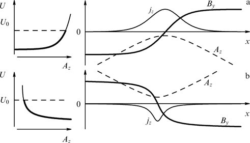
Figure 13. Typical Grad–Shafranov potential U(Az) and coordinate dependences of Az, By, and jz for: (a) the Harris sheet described by Eqn (122), and (b) solution (131), (132), analogous to the Harris sheet and described by Eqn (130).
Download figure:
Standard imageThe concentration will be finite only if function  decreases with increasing p faster than exp (−ζαp/mαc). Let us choose by way of illustration this function in the form
where kB and Tα are constants, the product of which has an energy dimension. (If kB is the Boltzmann constant, such a choice at ζα = 0 and nonrelativistic momenta transforms distribution (120) into the Maxwell–Boltzmann thermodynamically equilibrium distribution with temperature Tα.) Then, the distribution function fα assumes the form
where  . The distribution remains Maxwellian in shape, but its center in the momentum space is shifted by mαVα = kBTαζα/c toward pz maintaining the current with density proportional to particle concentration. The equality condition for all kinds of particles regarding the combinations ζαeα/mα suggests the equality of eαVα/Tα combinations; in other words, particles with different signs of the charge travel in opposite directions, thus making a contribution of a single sign to the current density.
It should be noted that the distribution of particles of each kind in a reference frame moving along the z-axis with velocity kBTαζα/(mαc) is the Maxwellian thermodynamically equilibrium distribution with the inhomogeneous profile maintained due to the fact that the plasma in this reference frame resides in the confining electrostatic potential. Designation of the momentum in this reference frame by  allows obtaining from expression (127) the equilibrium distribution in the electrostatic potential φ',
where φ' = AzVα/c, in excellent agreement with the Lorentz transform for nonrelativistic relative velocities of reference frames. Current sheet (124) with distribution function (127) is universally known as the Harris sheet [2]. The method proposed here using integrals of motion allowed performing generalization of the Harris sheet to arbitrary (including relativistic) values of momenta and arbitrary energy distributions defined by functions  onto which no limitations are imposed, except nonnegativity and a fast enough decrease with increasing particle momentum.
A current sheet analogous to the Harris sheet can be obtained for PDFs of the power-like form (88) at i = −1 (hyperbolic profile). Let us consider, for variety, a specific case of the planar layered distribution with py ≡ 0, i.e., with momenta lying in the xz plane, when the Grad–Shafranov equation appears in the form
The introduced function Rα, −1(p) admits a variety of particle energy distributions influencing the parameters of a current sheet.
Localized solution can be obtained even in the simplest monotonic case of Rα, −1(p) = Cα, −1cp0δ(p − p0), when
where Cα, −1 is a certain dimensionless constant.
Let us assume, for simplicity, that particles from all current-carrying plasma components have equal charge moduli and momenta; then the functional dependences of all terms in equation (130) are the same, and only multipliers are different. The Grad–Shafranov potential decreases monotonically and tends toward zero as Az increases from cp0/|eα| to infinity. Any value of Az = Az min satisfying the condition Az min > cp0/|eα| can be chosen as the 'turning point', i.e., the value of Az in the center of the current sheet where By = −dAy/dx = 0. The solution of equation (130) can be implicitly expressed in the form
Here, the x-coordinate is counted from the middle of the current sheet, and B0 is the magnetic field far from the sheet:
The form of the solution is demonstrated in Fig. 13b. It follows from the last formula that the maximum magnitude of the magnetic field is estimated as

For energy-dependent functions more complicated than the δ-function, the qualitative form of the solution remains unaltered and can be easily constructed numerically; however, an analytical solution like those defined by expressions (131), (132), even in the implicit form, contains more than one integral.
The isolated current sheet thus obtained differs from the known isolated Harris type sheets in that the particle distribution at its periphery becomes actually isotropic, while the current density decreases in the power-law fashion rather than exponentially.
3.2.2. Double-scale current sheets
Further generalization of the Harris current sheet is possible based on the PDFs with two exponential components having different coefficients of Az in the exponent. One can successfully obtain an analytical solution when these coefficients differ by a factor of two, i.e., the distribution functions have the form
where the functional factors  and
and  are the arbitrary functions responsible for nonnegativity of the particle distribution function (for the nonrelativistic distribution in the form (126), this means the presence of two Maxwellian components with momenta differently shifted in the direction of pz). In this case, the Grad–Shafranov equation acquires one more term, in comparison with equation (122):

and the Grad–Shafranov potential becomes equal to
Coefficient W2 is expressed via the integral with a certain weighting factor of a function  using an expression analogous to formula (121); it is small if component
  is minor. Equation (136) has the following family of aperiodic solutions:
where the spatial scale κ−1 is a free parameter. The profiles of a magnetic field and current density are expressed using the following formulas:
At W2 = 0, x0 = 0, formulas (138)–(140) turn into (123), (124). For W2 < 0, W0 > 0, the unbounded solution is either a partially or completely screened current sheet, depending on the value of the first integral  . In general, the current sheet is partly screened, while the magnetic field far from it is finite (Fig. 14a) and equals 2κA0, as in solution (124), whereas vector potential (138) has the asymptotic form Az ≈ −2A0|κx| at large x. In the limiting case κ → 0, the screening is complete (Fig. 14b):

Figure 14. Profile of the Grad–Shafranov potential (137) for W0 > 0, W2 < 0 and coordinate dependences of Az, By, and jz characteristic of: (a) a partly screened current sheet, U0 > 0, and (b) a completely screened current sheet, U0 = 0.
Download figure:
Standard imageThe magnetic field reaches the maximum value  at
at  (which is essentially a half-width of the current sheet; let it be denoted by D). Maximum current density is reached at x = x0 when it equals
It follows from the last relationship that the mean current density is half as much as its maximum value in the region of space with jz/A0 > 0, because (c/4π)By max = 2D〈jz〉r).
Moreover, equation (136) for W2 < 0, W0 > 0, unlike the case with a single exponent (122), has periodic anharmonic solutions
where the spatial scale k−1 is a free parameter. The limited scope of this review does not permit us to consider them in greater detail or to compare the results with the periodic solutions from Section 3.1.2.
There are no periodic solutions if W0 < 0. The general solution is described by the same formulas (138)–(140), but there is an upper bound on parameter κ (otherwise, the radicand would be negative):
The solution at κ close enough to this threshold, i.e., for minimal spatial scales of the sheets, is presented in Fig. 15a. In this case, the current sheet is split into two co-directional sheets, with the distance between them increasing closer to the k threshold (146), i.e., as U0 approaches the top of the Grad–Shafranov potential.

Figure 15. Profile of the Grad–Shafranov potential (137) for W0 < 0, W2 > 0 and the coordinate dependences of Az, By, and jz characteristic of (a) the split current sheet with U0 close to  , and (b) the symmetric transition sheet (from a homogeneous plasma to a vacuum with a uniform magnetic field; N is the particle concentration) realized at
  .
.
Download figure:
Standard imageIn the limiting case  , there is only one current sheet (to realize this limit passage, the quantity x0 must properly be tended toward infinity). It makes up the boundary between magnetized and nonmagnetized plasmas (other solutions of this type are considered in Section 3.4.3). Performing the limit passage, we get the solution presented in Fig. 15b:
where  is the arbitrary constant responsible for the position of the current sheet center.
An analogous case in which coefficients of Az in the exponents of distribution function (135) differ by more than twofold, e.g., w times, can be realized in the distribution of both particles of one type and particles of a multicomponent plasma where the distributions of particles of different kinds are described by simple functions (120) with markedly different values of combination ζαeα/mα and, generally speaking, different  functions. To be certain, let us consider the case of a multicomponent plasma containing two fractions of current-carrying ions with the distribution functions fi1 and fi2, respectively:
Here, ei1 and ei2 are charges on ions of two kinds (let them be positive), mi1 and mi2 are their masses, ζi1 and ζi2 are dimensionless constants, and  and
and  are nonnegative functions rather rapidly decreasing as p → ∞ [faster than p−4 exp (−ζip/mic), which ensures convergence of integrals defining current density and particle concentration].
Electroneutrality of the plasma can be achieved by negatively charged resting particles with the same spatial distribution as that of ions. Of greater interest, however, is the case in which neutrality is due to traveling electrons with the spatial distribution of the same class:
Here, ζe1 and ζe2 are dimensionless constants, the values of which are calculated below, and  and
and  are rather rapidly decreasing nonnegative functions.
On the assumption that the remaining plasma components (if any) do not create a space charge, the electroneutrality condition that must be satisfied at each point of space assumes the form

where ni1, ni2, and ne are the local concentrations of two ionic components and the total electron component. They are calculated on multiplying expressions (149), (150) by Ni1, Ni2, Ne1, and Ne2, respectively, and simply integrating over momenta that leads to the following relation:
where α = i1, i2, e1, e2. To recall, Ni1, Ni2, Ne1, Ne2 are constants having the dimension of particle concentration, and the necessity of their introduction is dictated by the choice of dimensionless functions fi1, fi2, fe1, fe2. Factors N and f always enter expressions for real physical quantities in the form of a product; therefore, the values of N and normalization of f functions are not stated here.
Thus, to satisfy the neutrality condition at all points (and at all Az values), suffice it to fulfill the equalities


which uniquely define the parameters ζe1, ζe2 of electron distribution function but preserve the freedom in choosing  functions determining electron energy distribution. These can be any rapidly decreasing nonnegative functions, each with a single integral limitation determining normalization. If the charge density of the electron component equals that of the respective ion component at a certain point, this equality is automatically fulfilled at all the remaining points. All this is equally true of relativistic and nonrelativistic cases.
It is worthwhile to note that distribution functions (149), (150) regarded as distributions over momenta at a given point are the same over the entire space to within the common multiplier. Here are a few examples of such distributions. To recall [see formulas (126), (127)], if  , the particle distribution in the nonrelativistic case matches the Maxwellian distribution with the shifted center in the momentum space, i.e., in the frame of reference where these particles create no current, with their distribution being isotropic and Maxwellian. For other types of
  functions, the distribution in the nonrelativistic case will not isotropic in any reference frame. Figure 16 illustrates particle distributions for
  , and
, and  , where η is a certain constant. Such 'crescent-shaped' distribution functions emerge in the measurements of particle distributions in current sheets in the tail of Earth's magnetosphere [210].
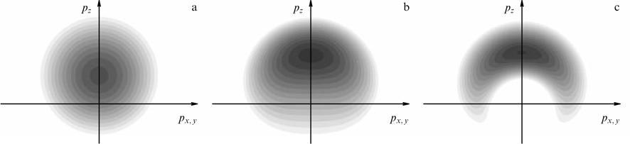
Figure 16. Examples of distribution functions in the form (150): (a)  ; (b)
; (b)  , and (c)
  .
.
Download figure:
Standard imageThe Grad–Shafranov potential is calculated as usual by taking a definite integral over momenta and an indefinite one over Az; in the case of interest, it results in
where
with W1 and W2 calculated using formulas analogous to (121):
Noice, without going into the details of the resultant solutions, that if w ⪢ 1 or w ⪡ 1 and both quantities W1 and W2 are positive, the current density profile can be a double-scale one, i.e., have the shape of current sheets of markedly different thicknesses embedded within each other, so that various kinds of ions make up current sheets of different scales. The example of such embedding is presented in Fig. 17.
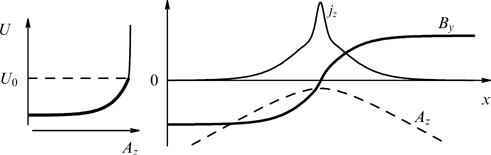
Figure 17. The profile of the Grad–Shafranov potential (137) for W0 > 0, W2 > 0, w = 30 and coordinate dependences of Az, By, and jz characteristic of a nested current sheet.
Download figure:
Standard image3.2.3. Exact solutions with singularities and symmetric periodic exact solutions
One of the variants of the Grad–Shafranov potential (156) for which equation (68) can be integrated to completion is the combination of parameters W1 = W2, w = −1 when U(Az) ∝ cosh (Az/A0). The solutions for Az(x) and W1 = W2 > 0 are written out via elliptical integrals, and some specific solutions via elementary functions for W1 = W2 < 0.
One such solution for W1 = W2 < 0 corresponds to the case in which the value of the first integral of equation (68) equals the maximum of potential U(Az):
Then,
where the value of x0 determines only the shift of the solution as a whole. The choice of x0 = 0 yields the following expressions for the magnetic field magnitude and current density:
It follows from the equality of the above By values as x → ±∞ that the total current over the entire space is zero, but the current density has the same sign everywhere according to formula (162). The causes of this discrepancy will be discussed below.
The periodic solution can also be written out analytically by changing the sign on the right-hand side of relation (159) and assuming W1 < 0 as before:
Relevant integration leads to the solution
For brevity, assume x0 = 0 as before. Expressions for the magnitude of the magnetic field and current density resemble formulas (161), (162), the only difference being the substitution of trigonometric functions for hyperbolic ones:
Solutions (160)–(162) and (164)–(166) differ from all those considered above in that they exhibit a singularity (in the vicinity of zero in the former case, and in the vicinity of points  at all integer n in the latter); namely, the magnetic field, current density, and particle concentration are unbounded. The behavior of these two solutions in the vicinity of zero is similar, despite some differences: Az(x) along with By(x) in both solutions tend toward each other as x → 0, while the difference between jz(x) (as between particle concentrations) in the two solutions tends toward a nonzero constant, as readily follows from the expansion of quantities (160)–(162) and (164)–(166) into series in the vicinity of point x = 0.
Because all the above equations hold only at finite values of all constituent quantities, it seems also appropriate to write out the boundary condition at the discontinuity point:
Function jz(x) being even, the formal value of integral ∫jz(x) dx at any given limits of integration does not depend on the mode of detour around the singularity at x = 0 in the complex plane, and any detour of this singularity produces the necessary jump on the left-hand side of the equality. However, the infinite discontinuity of the magnetic field makes necessary a flat countercurrent flow with infinite linear density for the boundary condition to be fulfilled at x = 0. It means that these solutions are nonphysical if considered in the region of space encompassing the singularity.
Furthermore, the exact analytical solution can be obtained for the equation
that corresponds, in particular, to the case in which particles forming structures described by equation (136) are supplemented by 'reverse flow' particles with the same dependence of their distribution function on the vector potential component Az, but opposite values of momentum projection pz and opposite charge sign. Here, we choose the sign of the item with an arbitrary multiplier W2 differently than in formula (136) to more conveniently write out solutions in which W0 and W2 will be assumed positive.
The respective Grad–Shafranov potential takes the form
and tends toward +∞ as Az → ±∞, suggesting the existence of nonlinear periodic solutions. One of them can be written down in elementary functions:
When W2 ⪡ W0, solutions (170), (171) are close to a harmonic one; for W2 ⪢ W0, the solution is strongly anharmonic, because the argument of hyperbolic arctangent can be close to ±1, which is analogous to the appearance of anharmonic sheets considered at the end of Section 3.1.2.
The Grad–Shafranov potential (169) has the shape of a potential well with a single minimum in the center for W2 < 2W0. For W2 > 2W0, there is a maximum in the center and two minima on both its sides at points
The shapes of the profiles of the magnetic vector potential, magnetic field, and current density for two different W2/W0 ratios are illustrated in Fig. 18.
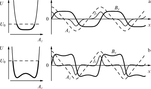
Figure 18. The profile of the Grad–Shafranov potential (169) and coordinate dependences of Az, By, and jz for the anharmonic periodic solutions (170), (171) at W2 = 2W0 (a), and W2 = 6W0 (b).
Download figure:
Standard image3.3. Polynomially exponential particle distributions
Let us now consider a more general case of PDFs in the form of the product of the exponent and polynomial:
for which the Grad–Shafranov potential in equation (68) has the exponentially polynomial form, too:
where the coefficients are determined by integrals:
of arbitrary functions  with the weight given by dimensionless expressions
Here, Γ(...,...) is the so-called incomplete gamma-function defined by the formula

It is connected with the ordinary gamma-function by the relation Γ(s, 0) = Γ(s). In the case of nonnegative integer i and l (i ≥ l) under consideration, the factor exp (b)Γ(i − l + 1, b) is an i − l degree polynomial in b. The expressions for an incomplete gamma-function for the five natural values of the first argument are written out in the explicit form as
In other words, in this case, too, we have the universal functional form of the Grad–Shafranov potential, while particle distribution functions determine only the set of its coefficients, even though they influence parameters of the resultant current sheets.
Another quite general case is represented by the distribution functions in which the exponent is quadratically dependent on the projection of the generalized momentum (a similar case was considered from somewhat different standpoints in Ref. [7]). It is appropriate to precede the general analysis by a description of the simplest variant with
where ζα are dimensionless constants, and  are certain yet arbitrary functions. Then, the equation for the vector potential (68) assumes the form
The integral over pz in the square brackets equals
where the error function was introduced:

Because the integrand contains special functions, further integration over p on the right-hand side of Eqn (180) cannot be performed analytically in the general case, although the analysis is possible in certain specific cases, e.g., when the weight factor  is the sum of δ-functions.
An important special case in which integrals can be removed from the Grad–Shafranov equation is the Maxwellian dependence of distribution functions on the particle energy, when  , where Cα and pα are constants. Integration yields the Grad–Shafranov potential in the form of the sum of exponentials with the exponents quadratically dependent on Az:
An analogous result can be obtained for the particle distribution function having a more general form:
with different Aα constants for different kinds of particles:
Let us turn back to the general case of the exponent additionally having a polynomial multiplier, besides the exponential multiplier with a quadratic form from the vector potential:
Integration in elementary functions is again possible for the case of  , where Cαi and pαi are constants (Lorentz factor γα depends on p). It is also possible, for generality, to write Az − Aα instead of Az with different constants Aα for different kinds of particles (we do not follow it for brevity). Then, we arrive at
It is easy to make certain that substitution of d = 0 into last expression yields formula (183).
The use of the general expression found for the Grad–Shafranov potential opens up ample opportunities for analytical construction of various self-consistent current sheets in the near future.
3.4. Nonsmooth particle distributions
3.4.1. Grad–Shafranov potential for localized current sheets in an external magnetic field
Let us consider, with reference to the description of current sheets in contact with the region occupied by an external uniform magnetic field, some nonsmooth PDFs that can ensure an appropriate shape of the Grad–Shafranov potential specified at the end of Section 2.5 in connection with the classification of possible planar layered solutions.
The simplest suitable example of a PDF for which integrals entering into the Grad–Shafranov equation (68) can be calculated analytically is provided by the particle distribution depending on the projection of the generalized momentum through the sum of δ-functions in the form δ((pz + eαAz/c − Pi(p))/mαc) with certain weights. Let us consider, as the dependence on the momentum projection py, the two simplest variants: one without an explicit dependence (cylindrically symmetric case with pz-axis), and the other with an explicit dependence in the form of a δ-function δ(py) (a case of planar layered particle motion).
The first variant is specified as
where Pi(p) are certain functions that can actually be chosen arbitrary, and  are arbitrary functions assumed to be nonnegative in order to assure PDF fα nonnegativity. Current density created by particles of a kind α is calculated by moving into the spherical system of coordinates in the momentum space and gives the following Grad–Shafranov potential:
where H(...) is the Heaviside step function.
The following distribution function is considered for the planar layered variant:
Current density is easy to calculate by moving to the cylindrical system of coordinates with the resulting Grad–Shafranov potential
Current configurations corresponding to a potential of such a form apparently have not yet been studied.
One more useful example of a PDF with the nonsmooth dependence on the projection of the generalized momentum is associated with the use of the modulus function
The density of current created by particles of a kind α is easy to calculate as
For example, the following expression is derived for the monoenergetic distribution  , where p0 is the modulus of the particle momentum equal for all particles of a kind α:
Evidently, the right-hand side of Eqn (194) is a smooth function of Az. Therefore, the Az dependence of jα and the respective profile of the Grad–Shafranov potential U(Az) are smooth, too, even in the case of the general form of the functional cofactor  , because the general form of current density jα can be obtained by integrating (194) over p0 with weight
  .
.
It is also possible to consider the nonsmooth distribution function of a more general form
for which the Grad–Shafranov potential is calculated and written out as
When eαAz > pc, the last expression is in excellent agreement with formula (89). Naturally, it is possible to take the distribution function in terms of several summands of form (195) with different values of power i and substitute in each of them eαAz/c by eαAz/c − Pi(p), where Pi(p) is an arbitrary function. By virtue of linearity, the corresponding formula for the Grad–Shafranov potential generalizing expression (196) is written out trivially.
Finally, let us consider the PDF, the dependence of which on the generalized momentum is determined by the Heaviside step function (its presence is quite natural in the description of the boundary between the plasma and the plasma-free region occupied by an external magnetic field):
Here, Pi(p) are certain functions that can be chosen, in essence, arbitrarily, and function  is assumed to be nonnegative as before to guarantee the nonnegativity of PDF fα.
The corresponding Grad–Shafranov potential can be reduced to
The integrand in the last formula (as a function of Az) equals a constant for eαAz/c < Pi(p) − p, and another constant for eαAz/c > Pi(p) + p; it is equal to the cubic function of Az between the two constants.
For a more general form of PDFs [functions Pi(p) are not written here, for brevity], viz.
the expression for the Grad–Shafranov potential can be written out taking advantage of linearity and the obvious relationship
Then, it follows from formulas (89) and (196) that
Evidently, potential (201) calculated at i = 0 differs from expression (198) at Pi(p) = 0 only by a constant, so that formula (201) can be applied not only for positive powers i, but also for the zero power.
3.4.2. Current configurations with distribution functions in the form of δ-functions in an external magnetic field
Let us consider the expansion of cylindrically symmetric distribution functions into δ-functions of the projection of the generalized momentum (188) and the respective Grad–Shafranov potential (189) in the monoenergetic case5 when  dependences also have the form of the δ-functions,
  :
:
Then, the current density (to be precise, its component for each concrete ith item) is linearly dependent on the vector potential within the interval from c(Pi(p0) − p0)/eα to c(Pi(p0) + p0)/eα (with derivative djα/dAz being negative) and equals zero outside this interval. The Grad–Shafranov potential (189) over the same interval has the shape of a parabola convex upwards with the vertex at Az = Pi(p). The parabola being convex upwards, the solution with a localized magnetic field in which the current is determined by a single kind of monoenergetic particles with one term in sum (188) is impossible to construct (a localized solution should be possible if there were two such parabolas with a 'potential well' between their vertices), and all solutions have the form either of a symmetric current sheet with an antisymmetric magnetic field (in analogy with the Harris sheet when the value of the first integral U0 is below the parabola vertex) or of an antisymmetric current sheet in an external uniform magnetic field (when the U0 value is above the parabola vertex) or the current sheet at the border between the homogeneous nonmagnetized plasma and the magnetic field (when the U0 value coincides with the parabola vertex in terms of height).
Let us analyze the latter case assuming, for brevity, that Pi = 0. Then, as Az → 0, i.e., in the depth of the plasma volume, the magnetic field tends toward zero, too, and the expansion of potential (189) in the vicinity of Az = 0 takes the form
with the result that in the linear approximation it leads to the homogeneous equation
solutions of which give the exponentially decaying profile of the vector potential and, therefore, of the magnetic field By(x).
If all current-carrying particles have an identical Lorentz factor γα, the integral in the last expression can be written out via the local particle concentration nα in the region where Az and the magnetic field are close to zero:
This means that the scale of magnetic field attenuation with penetration to the plasma interior is c/ωpα. Notice that the plasma is strongly anisotropic in this solution even in the uniform region.
Analogous symmetric, antisymmetric, and transition current sheets can also be constructed in a monoenergetic case for the flat distribution functions (190) on the assumption of  . Then, the item for each concrete i in the Grad–Shafranov potential (191) over the interval from c(Pi(p0) − p0)/eα to c(Pi(p0) + p0)/eα has the shape of a semi-ellipse (concave upwards), and vanishes outside this interval. For a given i at each point of the space, particles have a fixed total momentum p = p0, momentum projection py = 0, and projection pz = Pi(p0) − eαAz/c. This uniquely defines the remaining projection to within sign:
  , meaning that for a given i two symmetric particle trajectories pass through each point of space at which the Az value falls into the interval from c(Pi(p0) − p0)/eα to c(Pi(p0) + p0)/eα. There are 'turning points' at the interval boundaries in which px = 0 and the current density becomes infinite (the simplest current sheets with such a delta-shaped PDF for a boundary-value problem appear to have been considered for the first time in Ref. [155]).
The invariant method allows us to describe for such a PDF the structure of the boundary between a homogeneous two-beam plasma (analogous to that considered in Section 3.4.3) and a vacuum with a constant magnetic field. To this end, we take

for one of the items in sum (190), and  for the remaining ones, assuming for simplicity all Pi(p0) equal to zero. In so doing, the distribution function fα assumes the form
The Grad–Shafranov potential (191), written as
is equal to zero for  , and the radicand in expression (208) is negative. Because we wish to describe here the case in which part of the space is occupied by a homogeneous plasma without a magnetic field, we have to choose such a solution of the Grad–Shafranov equation at which derivative dAz/dx is zero at the potential maximum point, i.e., at Az = 0. For this purpose, the value of the first integral of the Grad–Shafranov equation should be chosen as Umax = U(0):
The plots of a magnetic field, particle concentration, current density, and electron trajectories for this solution are presented in Fig. 19.
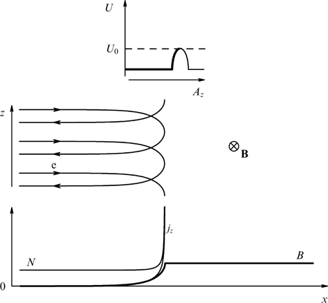
Figure 19. Grad–Shafranov potential (208), electron trajectories, and profiles of the magnetic field, current density, and particle concentration at the boundary of a uniform magnetic field and a two-beam plasma (at U0 = Umax).
Download figure:
Standard imageIn the regions with a weak magnetic field, i.e., in the vicinity of Az = 0, the potential can be expanded into a series:
whence [using relation (209)] it follows that
i.e., exponential decay of the magnetic field with penetration to the plasma interior.
Notice that in the solution thus obtained magnetic field magnitudes far from the current sheet as x → +∞ and x → −∞ differ not only in sign, which suggests the presence of a fraction of the 'external' field created by some currents flowing 'at infinity' that do not enter the system being described.
Let us calculate the local relationship between magnetic field energy density and particle energy density. It follows from expressions (207)–(209) that
where U0 is the value of the first integral of the Grad–Shafranov equation,  . The inequality
  is fulfilled except when the current structure of interest is in an external uniform magnetic field. With this inequality in mind, it follows from expression (212) that B < 1/4.
Let us make an analogous estimate in the general case when the current structure being considered contains particles with different energies and the Grad–Shafranov potential has the general form (191). Then, the relationship between local energy density of the magnetic field and that of the particles is written out as
where integration is purely real, and integrals are calculated only over regions with a positive radicand. Taking advantage of the fact that the weighted harmonic average of positive quantities does not exceed their arithmetic average, it is possible to write down the estimate
where  αi is the set of such p > 0 for which (eαAz/c − Pi(p))2 ≤ p2. Whence it follows that
Next, if the current structure of interest is not in the external uniform magnetic field, there is a point where the field (and B) vanishes. Bearing this in mind and taking advantage of relationship (213) we find the upper bound for U0 leading to the inequality
Notice that these estimates are exact in the sense that B values close to 1/4 are possible. The latter inequality from formula (216) holds true if distribution functions Fαi(p) differ from zero only inside αi set (otherwise, the magnetic field at this point would be formed by particles whose trajectories do not pass through the plane with the same x and it would be senseless to compare local densities of the current and magnetic field; in particular, in the situation depicted in Fig. 19, the magnetic field also exists in the region where there are no particles at all).
Figure 19 illustrates a case in which the value of U0 is exactly equal to the height of the Grad–Shafranov potential maximum:  . Let us consider in brief what happens if U0 is greater or smaller than this value. When U0 < Umax, the representative point reflects from the slope of the Grad–Shafranov potential profile, giving rise to a spatially localized current structure and an antisymmetric self-consistent magnetic field it creates, as shown in Fig. 20. The current density profile is symmetric, while the magnetic field density profile is antisymmetric. The width of the current structure can be either much greater than the gyroradius of particles in the magnetic field they create at infinity (at U0 close to Umax) or of the same order as the gyroradius, and even much smaller than that for U0 ⪡ Umax. In the last case, the particles travel largely along the z-axis and deflects from it only through small angles.

Figure 20. Grad–Shafranov potential (208), electron trajectories, and profiles of the magnetic field, current density, and particle concentration for a sheet with an antisymmetric magnetic field (for U0 < Umax).
Download figure:
Standard imageIf U0 > Umax, the representative point passes through the maximum of the Grad–Shafranov potential without stopping; such a situation corresponds to a localized current structure placed in an external uniform magnetic field, as shown in Fig. 21. The current density profile is antisymmetric, that of the magnetic field symmetric, and particles move along closed trajectories. The current structure has a width on the order of the particle gyroradius in an external field if U0 greatly exceeds Umax, and its width can be much greater than the particle gyroradius in an external field if U0 is close to Umax. In the latter case, the magnetic field in the structure center becomes much smaller than the external one.

Figure 21. Grad–Shafranov potential (208), electron trajectories, and profiles of the magnetic field, current density, and particle concentration for a sheet with a symmetric magnetic field (for U0 > Umax).
Download figure:
Standard imageSuperposing the two solutions presented in Fig. 19 yields the solution describing a two-flow plasma divided into two parts by the region with a magnetic field, as illustrated in Fig. 22.
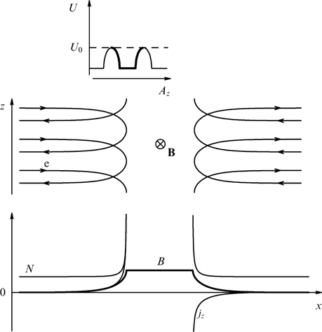
Figure 22. Grad–Shafranov potential, electron trajectories, and profiles of the magnetic field, current density, and particle concentration for two spatially separated fractions of particles (at U0 = Umax).
Download figure:
Standard image3.4.3. Boundary between an isotropic plasma and an uniform magnetic field
In the above examples of solutions describing the boundary between a homogeneous nonmagnetized plasma and the uniform region with a magnetic field, the plasma was essentially anisotropic at all points in space. Let us construct a solution in which the plasma is isotropic at the periphery of the sheet, taking the plasma PDF in the form of expression (197) with a single value of index i:
When a change in eαAz/c from negative to positive values is much greater than the mean value 〈p〉 of momentum, the Grad–Shafranov potential U(Az) (198) decreases by
so that magnetic field energy densities in a vacuum and a plasma differ by
i.e., by the magnitude of the gas-kinetic pressure of isotropic plasma, as expected. Let us assume in addition that the plasma in the homogeneous region is not only anisotropic but also Maxwellian, which simplifies analytical calculations and corresponds to the case of equilibrium distribution of practical significance:
Here, kB and Tα are the constants used above, the product of which has the dimension of energy, and the normalization factor in front of the exponential is chosen such that particle concentration nα in the region with a homogeneous plasma gives Nα when formula  is used for the calculation.
The Grad–Shafranov potential (198) in this case is expressed via the error function (182):
Accordingly, the magnetic field profile is described parametrically by the formulas
and the particle concentration profile can be found directly by integrating relationship (217) with the substitution of Maxwellian distribution (220):
It follows from formulas (223) and (224) that expression
is fulfilled and formally coincides with the equation of constancy of the sum of magnetic and gas-kinetic pressures in the magnetohydrostatics of isotropic plasma. The origin of result (225) obtained for a particular choice of the distribution function in the form (220) and for the particular way of 'cutting off' this function in accordance with expression (217) can be explained as follows. In the general case of a planar sheet, one has
Multiplication by By/4π = −(dAz/dx)/4π and integration over x give
Integrand (−jzBy)/c defines the density of the x-component of the force acting on the plasma from the magnetic field and equaling the difference of U/4π values at the edges of the plasma layer enclosed between planes x = x1 and x = x2 (this density is by definition the force acting on unit plasma area in the layer). In the static case of interest, this force must be equal to the difference between flux densities of the particle momentum x-component through unit area sites on planes x = x2 and x = x1. In the isotropic case, the flux density of the momentum component through a unit area site perpendicular to its direction can be identified with pressure. Distribution (220) is such that particle distributions over px and py at any pz = const are similar to within a pz-dependent common multiplier. Therefore, in 'cutting off' the distribution by plane pz = const according to expression (217), the relationship between the concentration and flux density of the x-component of the particle momentum remains the same as in the isotropic case: formula (225) contains nαkBT just as for an isotropic plasma.
To recall, although the function erf entering expressions (223) and (224) is antisymmetric with respect to Az, the magnetic field and particle concentration change at a different rate on either side of the plasma/vacuum interface. The reason is that the magnetic field in the plasma is weaker than in the vacuum (or even totally disappears), i.e., the value of dAz/dx is lower in the plasma. This means that the scale of a change, e.g., of current density (and therefore other parameters), is bigger with increasing distance from its maximum toward the plasma than toward the vacuum. The profiles of particle concentration, magnetic field, and current density for a nonmagnetized plasma/vacuum interface are exemplified in Fig. 23.
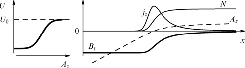
Figure 23. Profile of the Grad–Shafranov potential (221) and coordinate dependences of Az, By, jz, and N for solutions (222)–(224) corresponding to an asymmetric current sheet at the plasma/vacuum interface with a uniform magnetic field.
Download figure:
Standard imageThe form of transition between an isotropic Maxwellian plasma and a vacuum with a uniform magnetic field described by formulas (222) and (223) and shown in Fig. 23 is not the sole possible one. This inference follows from the fact that Pi(p) in the argument of a step PDF (197) can be taken differently than in formula (217). Specifically, the particle distribution assumes the form

in the case of the linear addition −μp, where μ is a constant with the modulus smaller than unity, while the plasma remains isotropic as eαAz →∞ and the number of particles at high negative values of eαAz is exponentially small. In this case, the integral in expression (198) is taken as well for Maxwellian distribution  (220); in other words, the form of the Grad–Shafranov potential U(Az) can be expressed analytically, but it is too cumbersome to be presented here.
A simpler way to describe the transition between a Maxwellian plasma and a vacuum differently from that given by formulas (222), (223) is to use in distribution function (197) two similar items instead of one with identical Maxwellian distributions  but different p-independent 'cutoff' P1 and P2 values. In this case, the Grad–Shafranov potential U(Az) will be the sum of two erf functions shifted along the Az axis, the magnetic field and particle concentration profiles remain monotonic even if of a more intricate shape than that described by formulas (222)–(224), and the current density profile has, at a large enough difference between P1 and P2, two maxima of distinct widths, as shown qualitatively in Fig. 24a.
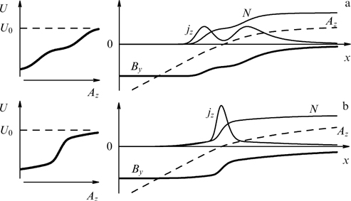
Figure 24. Typical profile of the Grad–Shafranov potential and coordinate dependences of Az, By, jz, and N: (a) for an asymmetrically split current sheet corresponding to distribution function (197) with two Maxwellian items with identical temperatures but different P1 and P2 'cut-off' positions, and (b) for a double-scale current sheet corresponding to distribution function (197) with two Maxwellian items of substantially different temperatures.
Download figure:
Standard imageAssuming P1 = P2 and using Maxwellian functions with notably different temperatures as  and
and  give the Grad–Shafranov potential in the form of the sum of two erf functions of different widths and current density profiles comprising a central narrow component and two wide tails on both its sides (see the example in Fig. 24b). Naturally, the 'wide' and 'narrow' components can be formed by plasma particles of one or two different kinds.
Although we considered above boundary between the isotropic nonmagnetized plasma and the vacuum, the same solutions hold for the interface between two regions of isotropic plasma with different magnitudes of the magnetic field, provided an isotropic plasma component with Maxwellian or non-Maxwellian energy distribution is added.
It is quite natural to use nonsmooth distribution functions for the description of such phase boundaries, taking into account the self-consistent field of transition current sheets, as is confirmed by their profiles presented in the figures. To recall, the simplest solutions of this type provided a basis for the elaboration of the kinetic theory of self-consistent current sheets [155, 158, 211]. Analytical solutions for transitional layers at the boundary between plasma and smooth distribution functions are possible, too, but remain to be more thoroughly explored.
4. Possible applications of exact solutions to the interpretation of observed current structures and results of their numerical simulation
The current level of the analytical understanding of self-consistent current structures facilitates further progress in the interpretation of their detection and observation, e.g., in the near-Earth and solar plasma, experiments with laser plasma, and adequate treatment of the results of numerical simulations of plasma processes associated with self-consistent magnetic fields, such as reconnection of magnetic field lines, current sheet structure in the presence of a few fractions of transit and trapped particles, and plasma confinement at the border with a strong magnetic field region.
Recently, special interest has been shown in modeling the formation of collisionless shock waves in which the generation of self-consistent magnetic fields plays the primary role [54, 56, 60, 85, 96, 212]. Results of some relevant numerical simulations give evidence of long-lived current filaments that slowly merge together and gradually grow in volume at and behind the shock wave front [44, 104, 212–214].
It was recently shown based on the results of numerical simulations [55, 67, 98, 215] that modern experiments with laser plasma provide conditions for the formation of collisionless shock waves. The very first such experiments have already given promising data suggesting the possibility of studying processes of magnetic field generation and current filament dynamics under these conditions [215]. In what follows, we do not touch on the shock wave problems, bearing in mind the complex behavior of filament ensembles, but focus on the problems of current structures and realization of their individual manifestations.
4.1. Specific features of current configurations leading to reconnection of magnetic field lines
Let us start with a description of current sheets and filaments giving rise to the reconnection of magnetic field lines. This phenomenon appears to have a collisionless character, which makes difficult its reproduction and observation under experimental conditions.
Experimental studies of this phenomenon in laser plasma have become possible quite recently [46, 68, 216–218]. An example of the magnetic field structure evolution conditioned by the formation of current filaments in a laser plasma flow is presented in Fig. 25. As far as a laboratory (nonlaser) low-pressure plasma created in large traps (e.g., MRX, RSX, TC-3D, KI-I) is concerned, the resolution of the spatial–temporal dynamics of the magnetic field on collisionless scales in such plasma is still insufficient for the in-depth investigation into details of the formation and evolution of self-consistent current structures (see, e.g., Refs [61, 64, 65, 70, 219, 220]). Nevertheless, experimental studies along these lines continue (one of the results is presented in Fig. 26). Anyway, the plasma thus obtained can be highly nonequilibrium and the initial current sheets have a far from Maxwellian PDFs.

Figure 25. Evolution of the magnetic field structure associated with the development of Weibel instability in laser plasma flows and observed by proton-emission tomography (a) in experiments [217, 218, 235] on a picosecond time scale at the flow periphery, and (b) in experiment [68] on a nanosecond time scale in the region of the intersection of two flows.
Download figure:
Standard image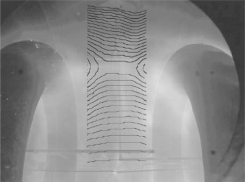
Figure 26. Typical plasma distribution (as a background) and magnetic field lines (cross section) in the vicinity of the current sheet formed in the force lines reconnection region (MRX facility, Princeton, www.pppl.gov) [46, 236, 237].
Download figure:
Standard imageRecent observations of current sheets in the magnetospheric plasma also show that they may have a non-Maxwellian PDF and differ for different kinds of particles, while the spatial structure of the current density is asymmetric, indented, and multiscale and, in particular, contains split and nested current sheets (see Section 4.2). Such observations are exemplified by satellite data concerning with current sheets in the tails of Earth's and Jupiter's magnetospheres [17, 34, 193–195, 221–225]. The diversity of PDFs and spatial magnetic field configurations associated with self-consistent current structures also appears to be natural in the astrophysical plasma, including active areas of the chromospheres and magnetic star coronas, current sheets formed by the stellar wind, or during contacts between magnetized plasma regions with different directions of the magnetic field in double systems with accretion (accretion disks and jets corresponding to neutron stars and black holes) (see, e.g., Refs [47, 57, 226–230]).
In all the above systems, reconnection of magnetic field lines is the most interesting and extensively discussed phenomenon (see, e.g., Refs [61, 231–234]). The process of reconnection, interpretation of the relevant data, and comprehension of the results of numerical simulations strongly depend on the initial configurations of current sheets or filaments and PDFs correlated with them. However, the initial current structures have thus far been taken in the form of Harris sheets and Bennett pinches (or their generalizations), while PDFs in the form of one- or two-temperature Maxwellian distributions, including those shifted by the hydrodynamic velocity of the flow of the corresponding particle fraction. At the same time, in accordance with Sections 2 and 3, the analytical representation of the self-consistent initial conditions is possible for a much wider class of configurations of the magnetic field, current, and PDF. The self-consistent particle energy distribution can be chosen to be essentially arbitrary and non-Maxwellian, even for Harris or Bennett type structures, which may help to more adequately take into account the physical conditions preceding reconnection.
This makes it possible to estimate if and how the process of reconnection depends on the initial current sheet and filament profiles and the initial PDF correlated with them. Of special interest are the reconnection rate, efficiency of generation of accelerated particles and waves in the plasma, current configuration parameters, and PDFs after completion of the process. Taken together, these characteristics could promote understanding the physical nature and effects (either observed or expected) of the reconnection of magnetic field lines in current sheets or filaments under laboratory and extraterrestrial conditions.
4.2. Double-scale and split current sheets in a magnetospheric plasma
Another class of topical problems requiring variability of PDFs and related current profiles pertains to the elucidation and interpretation of the intricate structure of current sheets in certain regions of the magnetospheres of Earth (Fig. 27), the Sun, and Jupiter.
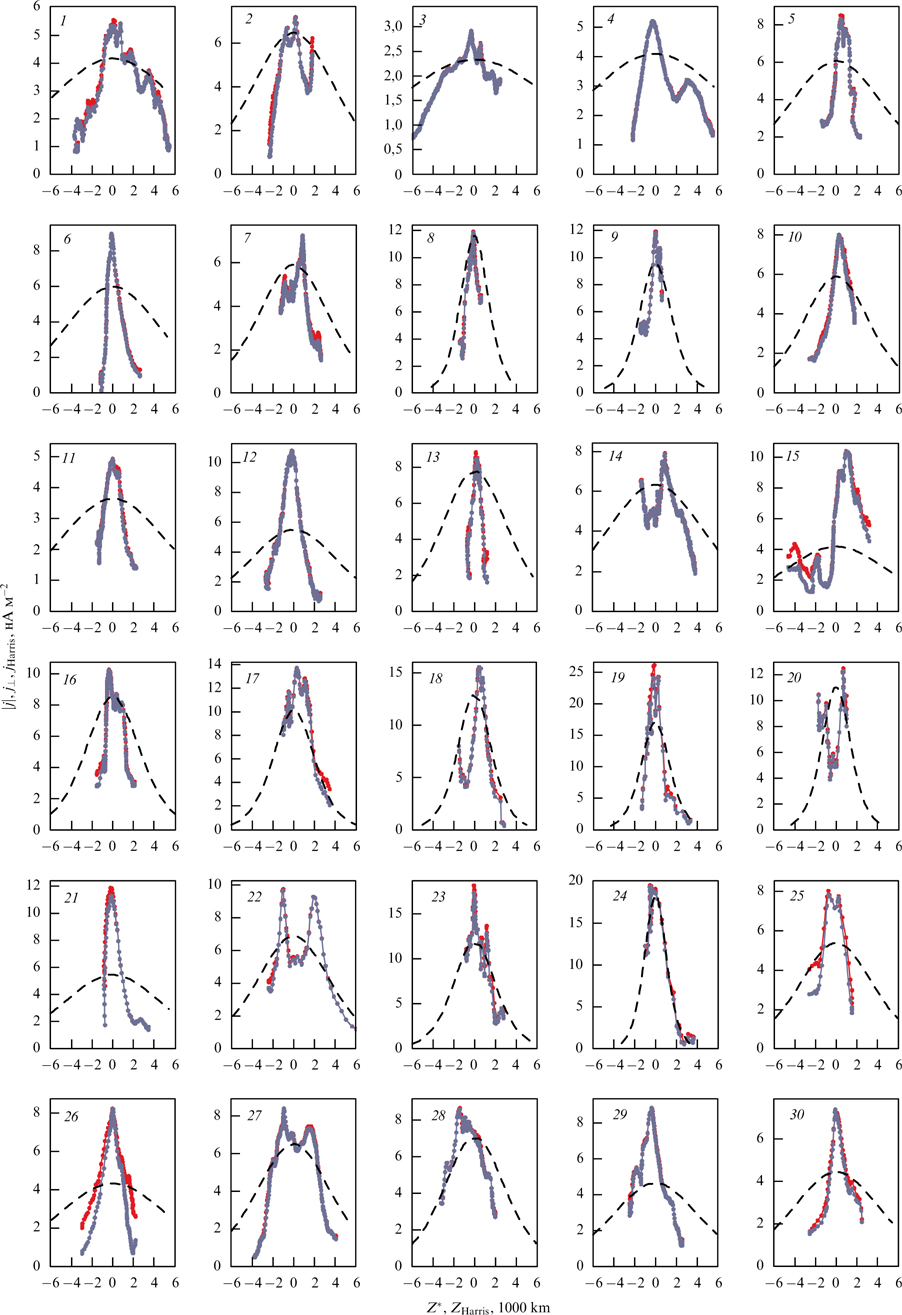
Figure 27. (Color online.) Current sheet profiles [dependences of current density j (blue curves) and its transverse component j⊥ (red curves) on the effective height] observed by the Cluster system of satellites [221]. The dashed line corresponds to the model Harris sheet.
Download figure:
Standard imageAs far as the Sun is concerned, these are in the first place the sites of plasma energy accumulation in the regions with strongly nonuniform directions of the magnetic field, in which coronal flares occur from time to time [47, 72, 76, 238, 239], as well as the regions of the warped heliospheric (equatorial), current sheet that, according to data from Voyager-1 and Voyager-2 missions, also exhibit activity, most probably due to the same phenomenon of reconnection of magnetic lines of force [240–242]. In both cases, there are grounds to suppose the existence of long-lived two- and many-humped (indented) current sheets with changing signs of the current and the magnetic field, although the structure and character of their PDFs remain unclear.
Somewhat better known are the so-called double-scale and split current sheets observed in the tail of the terrestrial atmosphere by near-Earth spacecraft, such as Geotail, Cluster, Interball, THEMIS, and MMS [17, 34, 45, 73, 74, 77, 222, 225]. It was shown that PDFs in these current sheets are anisotropic and, generally speaking, non-Maxwellian, e.g., two-temperature, functions significantly different for various ion and electron fractions. These sheets are very stable despite (or owing to?) external perturbations in the form of slowly changing magnetic fields and external fluxes of particles eventually attributed to a solar wind. The structure of the current sheets strongly depends on the fraction of trapped particles and the character and ratio of various ion fractions of transit particles. Trajectories of different particles can be altogether different, while accumulation or depletion of selected ion fractions may promote additional evolution of current sheets.
The reader is referred to numerous reviews for more detailed information about this issue (see, e.g., reviews [34, 35, 77] and references cited therein). Notice also that the data obtained during the Voyager-2 and Galileo space missions give evidence that a split current sheet can just as well emerge in the Jovian magnetosphere; curiously, the thickness of the double sheet can be smaller than that of a monolayer [194, 195].
The origin of split current sheets remains a mystery, and their analytical description is based either on a few modifications of the Maxwellian distribution, different for various ion fractions and responsible for the anisotropy of their pressure in the plane orthogonal to the magnetic field or on various numerical (MHD and PIC) models appealing to the simplest generalizations of the Harris sheet and Maxwellian PDFs. The extension of the class of analytical models of intricately structured current sheets, demonstrated in Sections 3.1–3.3, may significantly facilitate solving the problems under discussion.
4.3. Current structures with an external magnetic field at the boundary of two plasma regions with different parameters
One more long-standing important issue is the description of the boundary between the collisionless plasma and the region occupied by an external (given) magnetic field practically free of plasma [8, 155, 158, 186, 211]. In a more general setting, the problem reduces to the structure of the border between two half-spaces occupied by a homogeneous plasma with different parameters and containing an external magnetic field assumed to be uniform for simplicity. In the planar layered geometry, the transition current sheet creates own uniform magnetic field in the exterior to its volume and thereby weakens the magnetic field in one half-space, while strengthening it in the other. Generally speaking, a given particle flow can pass through the sheet but an analytical description of self-consistent current sheets has not yet been undertaken under such an aggravated condition; therefore, it is not discussed here. As shown in Section 3.4 based on a model PDF, transition sheet profiles in the external magnetic field can vary considerably but always obey the balance equation (58) and account for the plasma gas-kinetic pressure drop equaling the difference between magnetic pressures on either side of the sheet. It follows from Sections 2.2 and 2.6 that even more natural configurations of the transition sheet with the shear of magnetic field lines are possible.
The data suggesting the emergence of such structures in Earth's magnetosphere are presented in a number of reviews, e.g., Refs [45, 75]. Laser plasma experiments thus far permit the study of current sheets at the plasma–magnetic field interface only at the initial nonstationary stage of their formation. It was mentioned in the two preceding sections that theoretical analyses of such problems are usually based on highly limited kinetic models of transition layers either in the MHD approximation or by PIC simulations [8, 68, 186, 243–245]; hence, the necessity to further extend the class of analytical kinetic models of transition current sheets.
Unfortunately, we are aware only of nonsmooth PDFs allowing arbitrary energy distribution of particles in the analytical description of transitional current sheets. Although it is still very difficult to form a clear view of possible profiles and typical PDFs for transition sheets, the solutions obtained in Section 3.4 give reason to believe that such sheets can be highly diverse, viz. asymmetric, multiscale, with variable current density directions, etc. Anyway, a rather abrupt transition with the scale on the order of the gyroradius of typical particles in the sheet is possible from the strong magnetic field layer with a rarified plasma into the lower field region with a practically isotropic PDF. Such sheets, sometimes referred to as 'thin', are creating a great deal of interest [34, 35] stirred up by hopes for further progress on the analytical theory in this area.
4.4. Spectral and angular properties of synchrotron radiation of current sheets with power-law energy distributions of particles
Analytical expressions for an anisotropic PDF with an arbitrary enough energy dependence allow us to find out regular qualitative patterns in the properties of self-consistent current configurations related to peculiarities of the angular distribution of various energetic fractions of particles. This concluding section of the review deals with one such important property of relativistic self-consistent current sheets as their synchrotron radiation in the intrinsic magnetic field created by emitting particles (electrons) themselves. In this case, as opposed to an external uniform magnetic field common for the theory of synchrotron radiation, the particle distribution must inevitably be anisotropic for creating the current that maintains a self-magnetic field. As a result, certain (additional) anisotropy is imparted onto current sheet radiation. This feature is paramount when information about anisotropy of the observed synchrotron radiation spectrum is needed to characterize the anisotropic distribution of emitting particles, e.g., for diagnostics of the relativistic plasma and magnetic fields of various astrophysical objects, such as relativistic jets, collisionless shock waves, and equatorial current sheets formed by the pulsar wind in the neutron star magnetosphere [57, 58, 68, 95, 97, 98, 218, 235, 244, 246–253].
For certainty, we confine ourselves to the multipower-law particle energy distribution characteristic of a variety of situations in a nonequilibrium relativistic plasma and regarded as uniquely corresponding to the multipower-law synchrotron radiation spectrum [254, 255]. Our primary objective is to demonstrate differences in the emission pattern of an ensemble of particles forming the self-consistent magnetic field and an analogous isotopic ensemble of particles with the same energy distribution, placed in an external magnetic field with the strength of the same order of magnitude as the maximum strength of the field of the magnetostatic structure being considered. To this end, we shall lean upon the analysis of current sheets with the polynomial Grad–Shafranov potential made in Section 3.1 and compare the emission of particle ensembles with two distribution functions in the form of superposition of three consistent components exhibiting the power-law dependence on the generalized momentum with indices 0, 2, and 4 in the self-magnetic field and of superposition of the corresponding angle-averaged power-law components depending only on the energy in the external magnetic field [256]. Let us show that the spectrally angular differences in emission of these two ensembles are significant for a wide range of the ratios of coefficients of the above power series expansions, e.g., the number of spectral breaks can be different. Generalization of this example leads to the conclusion that the spectrum of intrinsic radiation coming from self-consistent current sheets in the relativistic plasma observed at different angles may contain a varying number of dominant power-law components, part of which are absent among dominant power-law components of self-radiation emitted by an isotropic ensemble of particles with the same energy distribution.
Let us consider as a model an antisymmetric neutral current sheet inhomogeneous along the x-axis, in which the magnetic field is directed along the y-axis, while vector potential and current along the z-axis. Let electron distribution be a polynomial function of the projection of the generalized momentum onto the z-axis and Lorentz factor γ in the interval (γmin, γmax):
Here, the exponent α and coefficients Hij of expansion are constants.
Let us confine ourselves for simplicity to the case of d = 4, assuming Hij = 0 for the odd indices i or j. This means that the current structure of interest is characterized by six coefficients, H00, H02, H04, H20, H22, H40, and one power-law symbol, α (the condition α > 13/3 needs to be fulfilled for some further calculations). Some of the Hij coefficients can be negative, but their choice is limited by the condition of nonnegativity of distribution function (229) for all Lorentz factors within the (γmin, γmax) interval and all electron velocity directions. Explicitly introducing the polar angle θ between the electron velocity direction and the z-axis (current direction) allows this distribution to be written as the sum of items with different powers of the Lorentz factor:
Let us assume that the optical thickness of the current sheet is much smaller than unity, and the refractive index of the rarefied plasma forming this sheet is close to unity. Then, its emission in the frequency interval (ωmin, ωmax) with boundaries  is determined by the sum of synchrotron emissivities corresponding to individual power-law distribution components with the spectral index ν:
  , where i = 0, 2, 4. To recall, a relativistic particle (with γ ⪢ 1) largely emits into the narrow cone of angles around the intrinsic velocity: for the frequency interval within which the radiation power is concentrated, and the spectral intensity of emission into the unit solid angle exponentially decreases as a function of the angle between the velocity and the direction of observation if this angle exceeds γ−1 [162]. As is well known (see, e.g., [257, 258]) this means that the anisotropy of synchrotron radiation is inherited from the anisotropy of particle distribution over momenta, and the emissivity of the plasma current sheet per unit volume at a frequency ω takes the form [254, 255]
Here, χ is the angle between the magnetic field and the direction of observation, ωB = |eB sin χ/mc| is the effective gyrofrequency, and M is the ν-dependent multiplier:
where Γ denotes the gamma-function and it is assumed everywhere that inequality ν > 1/3, to which the aforementioned restriction on α relates, is fulfilled.
Thus, the emissivity characterizing the current sheet to within the frequency-independent factor has the form
i.e., it breaks down into three power-law components with amplitudes:
The anticipated antisymmetric spatial dependence of the current density and the related vector potential component Az are derived from the Grad–Shafranov equation (see Section 3.1) with the bi-quadratic potential, with Hij = 0 for odd i due to asymmetry, and convenient calibration of the vector potential at which its zero value corresponds to the maximum magnitude of the magnetic field. With this in mind, all the items with odd exponents of Az were omitted above, since their contribution to radiation all the same disappears after integration over the sheet. Moreover, we do not consider, for brevity, emission from regions in which the magnetic field is much weaker than the maximum one, and which make only a negligible contribution to the total radiation that does not qualitatively alter its spectrally angular properties.
Each of the three items in the emissivity (233), (234) has an inherent angular dependence, while the direction of observation determines the characteristic frequencies,
at which contributions from the first and second or the second and third items become equal, i.e., spectral breaks occur. At certain directions of observation, some power-law components of the emissivity do not appear at all. For example, the amplitude of the intermediate item in a1 is low when the vector potential component Az is small and the condition cos2 θ ≃ −H02/H20 ≤ 1 is fulfilled. However, the role of such a component in the formation of radiation in other directions may be fairly well apparent.
The presence of 'hidden' components in radiation corresponds to the situation in which one of the items ai in the synchrotron emissivity aω is small enough after averaging over the solid angle:  . The particle distribution over energies (or over values of Lorentz factor γ, which is the same thing) obtained from distribution (230) averaged over the solid angle does not contain a component proportional to γ−α+2i and matching the aforementioned ai. At the same time, such a latent component unrecoverable by analysis of particle energy distribution can predominate at certain observation angles in a logarithmically wide frequency range.
This assertion can be exemplified by a spatially periodic or localized current sheet for the particles of which the middle component in the energy distribution is small (hidden), as in the case of fulfillment of the conditions H20 ≃ −3H02 and H22 ≃ −2H40. The intermediate component of emissivity
disappears upon averaging over the solid angle, but may be noticeable at observation directions given by angle θ for which cos2 θ is sufficiently far from 1/3. The range of such angles is determined by the inequality  , where w = ω2/ω1 is the ratio of frequencies ω2 and ω1 introduced above in formula (235) to serve as the upper and lower bounds of the spectral region where the intermediate component makes a dominant contribution to the emission.
For a planar spatially periodic current sheet with positive coefficients H00, H20, H40, and H04, this condition of dominance of the item a2 takes the form
(Because the main contribution to emission comes from the regions with a close-to-zero vector potential, this inequality is unrelated to the concrete shape of the periodic current sheet profile.) Here, μ = M2(α − 2)/M(α)M(α − 4), and  .
.
The nonnegativity of the PDF for all values and directions of particle momenta is assured by satisfying inequalities κ0 ≥ 1/36 and H04/H40 ≥ 1. If the values of these relations for distribution parameters are roughly twofold different from the bounds indicated and the typical values of index α = 5 − 10 (corresponding to μ ≃ 0.25 − 0.75), the intermediate component disguised by angular averaging predominates in the angle intervals θ ≲ 30° and 180° − θ ≲ 30° for a logarithmically wide frequency range (for w ≳ 10). For observations at nearly cross angles θ (to be precise, for cos2 θ ≲ 1/3), the frequency dependence of the emissivity in the (ωmin, ωmax) range contains only one break.
For small angles θ, i.e., for directions of observation close to the current direction, this dependence exhibits two breaks spaced far apart: ω1 and ω2, with the item a1 dominating between them and the power-law emission spectrum characterized by index (3 − α)/2 corresponding to the component with index 2 − α absent in the particle energy distribution. Frequency regions dominated by individual power-law components of synchrotron emissivity depending on observation angles are plotted in Fig. 28.
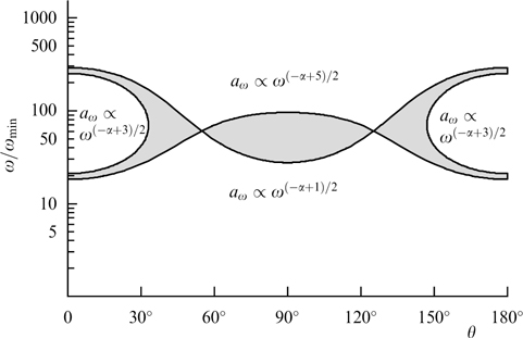
Figure 28. Frequency regions dominated by individual power-law components of synchrotron emissivity aω (233) depending on the direction of observation characterized by the polar angle θ with respect to current direction. The plots are constructed for the case of a spatially periodic current structure with a PDF in the form (229) at which angular averaging conceals the intermediate emission component a1. More than half of the total contribution to aω comes from the dominance criterion. Transition regions where it is impossible to distinguish a single dominant component are colored. Frequencies are plotted on the vertical axis in the logarithmic scale. Values of the parameters are as follows: α = 7.5, κ0 = 1/25, and H04/H40 = 2.
Download figure:
Standard imageConditions for the dominance of the 'latent' item a1 for a localized current sheet are considered in much detail in Ref. [256]. Such a sheet is possible for particle distribution (230) if two coefficients H20 and H40 are negative, and the remaining ones positive; then, the profile of the self-consistent vector potential is monotonic: Az = Amax tanh (x/x0), where the maximum value is given by the equality (eAmax/mc)2 =  . The intermediate item a1 can make a weighty contribution to the emissivity (231) for a logarithmically wide frequency range (ω1, ω2) in observation directions close to the perpendicular one with respect to the flowing current, i.e., θ ∼ 90°. In these directions, the spectrum has two breaks again (rather than one, as in the remaining directions), though the particle energy distribution has only two power-law components with indices −α and 4 − α.
A situation is also conceivable in which the power-law component with index 4 − α is missing in the energy distribution of particles and the corresponding major power-law component of emissivity a2 proves to be 'hidden': 〈a2〉θ ≃ 0. This scenario is realized if the condition H22 ≃ −3(H04 + H40/5) is fulfilled. It is easy to show [256] by analogy with the above cases that the 'hidden' radiation component a2 may prevail by virtue of particle distribution anisotropy, a2(θ) > |(3ωB/ω)a1(θ) + (3ωB/ω)2a0|, in a wide frequency range for a sufficiently wide cone of angles along the current with the opening up to 30°, depending on the parameters of the sheet.
To conclude, the frequency-angular spectrum of synchrotron radiation coming from self-consistent current structures (without an external magnetic field) in a relativistic collisionless plasma with the multipower-law particle energy distribution may contain breaks, extrema, and other features absent in radiation emitted by an ensemble of the same particles with the angle-averaged momentum distribution placed in an external uniform magnetic field. Depending on the angle of observation, emission of a self-consistent structure may have a different number of power-law frequency components prevailing in certain spectral intervals. This number can be higher than the number of power-law components in the particle energy distribution (averaged over angles), which suggests the generation of synchrotron radiation by the particles forming a self-consistent current structure rather than those arriving from an external region and characterized by mismatched energy distribution.
5. Conclusions
Construction of the theory of self-consistent configurations of the magnetic field and currents in a collisionless plasma is one of the most important problem in basic plasma physics, affecting, among other things, realization of far-reaching experiments with the so-called high-energy density laser plasma based on modern superpower lasers and elucidation of intriguing astrophysical phenomena (quasars, microquasars, stellar and pulsar wind, cosmic gamma-ray bursts, etc.) and events in near-space (shock waves and current sheets in the Sun's and planets' magnetospheres) that are becoming increasingly more observable using unique space vehicles and telescopes.
This review demonstrates that the use of invariants of particle motion in a collisionless multicomponent plasma (both relativistic and nonrelativistic) makes it possible to construct and analytically consider an extensive class of nonlinear neutral current structures (localized and not localized), including planar layered, cylindrically symmetric, and two-dimensional ones as exemplified by axially symmetric anisotropic PDFs in the momentum space, with the found static solutions allowing practically arbitrary particle distributions over energies. This implies the possibility of describing self-consistent sheets and filaments irreducible to usually employed models of the neutral Harris sheet and Bennett pinch or their known generalizations that actually exploit the Maxwellian distribution not always inherent in nonequilibrium collisionless plasma.
We proposed special expansions of particle distributions as the functions of projections of their generalized momenta onto the current direction in self-consistent magnetostatic configurations, including exponentially polynomial, delta-shaped, step, and other functions of particle motion invariants that make possible an in-depth investigation into solutions of the resultant nonlinear Grad–Shafranov equation. It enabled us to present the classification and analytical description of a variety of spatial profiles of stationary currents and magnetic fields to show that they are to a large extent arbitrary, too. This approach permits us to obtain analytical solutions for such current structures as double-scale and split ones possessing zero and finite total current, placed in an external magnetic field and bounded only by the intrinsic magnetic field. Some of the known solutions obtained for a narrow set of the simplest PDFs, including the Harris sheet, were generalized for the arbitrary relativistic particle energy distribution and configurations with the magnetic field shear.
Broadly speaking, studies on various classes of solutions of the Grad–Shafranov equation are still in the very early stages but look highly promising, first of all for the interpretation of various self-consistent current structures in laboratory and cosmic plasmas. The method for the construction of self-consistent current structures with an arbitrary energy distribution of particles, described in the review, considerably extends the understanding of magnetostatic structures in a collisionless plasma and provides a basis for the analysis of their dynamic properties, including large-scale instabilities and quasistationary interactions, as well as magnetostatic turbulence (by analogy with Langmuir wave turbulence and the turbulence of self-focusing channels of electromagnetic waves [259–266]).
To sum up, there is a representative but not exhaustive list of problems awaiting further research:
- (1)How representative are distribution functions depending only on particle motion invariants compared with a variety of distribution functions describing all stationary self-consistent current structures? How adequately do the first distributions represent qualitatively (physically) similar current structures described by more general particle distributions?
- (2)What self-consistent current structures are most (or least) stable and what is the hierarchy of their instabilities? For which particle distribution is the structure with a given current density profile most stable?
- (3)To what degree do the classes of stationary current structures extend (or contract) under the effect of a magnetic field imposed, for example, across the current sheet and/or boundary conditions, e.g., in prescribing the input and output particle flows at the borders of the current structure?
- (4)Is there a possibility of quasi-adiabatic (slow) deformation of current structures without their appreciable destruction and, if yes, under which conditions does it occur? Is it possible to macroscopically describe any current structure deformation or their interaction with each other without a detailed analysis of PDF evolution?
- (5)How do interparticle collisions, quasi-stationary electric fields, and higher-frequency electromagnetic fields influence self-consistent current structures? When does this influence result in their destruction or evolution of their macroscopic parameters without destruction, even if with a loss of energy content?
This list illustrates the complexity of the problem of self-consistent current structures and emphasizes the necessity of the development of new approaches to the investigation of its different aspects.
Acknowledgments
This study was partially supported by RSF grant No. 16-12-10528 (Sections 3 and 4) and conducted in the framework of the basic research program No. 15, Plasma Processes in Space and Laboratory, of the Physical Sciences Division, RAS, and under the State contract with IAP RAS (project 16.29) (Sections 1 and 4).
Footnotes
- 1
In the degenerate case, such a 'motion' ends at the point with zero-valued first and second derivatives of U(Az) with respect to Az (in analogy with the one-dimensional planar layered variant in Section 2.5). The infinitely slow monotonic approach to the bottom of the potential well is impossible: the general solution of Eqn (70) with a zero right-hand side has the form Az = c1 + c2 ln ρ; therefore, the motion is not restricted even for the absolutely flat bottom of the well, and 'friction' proves insufficient to stop the particle at a finite distance.
- 2
This criterion was obtained ignoring the magnetic field and does not allow possible instabilities with scales greater than or of the same order as the particle characteristic gyroradius to be judged. Therefore, instability of perturbations with scales in the range from the characteristic gyroradius rH to the characteristic inhomogeneity k−1 in fields of equipartition order awaits clarification. The problem of stability of long-wave perturbations with greater than k−1 scales just as well needs to be additionally considered taking account of structural inhomogeneity. A numerical analysis seems to be required to investigate, in general, the stability of both the simplest self-consistent current structure (see above) and more complicated structures (below).
- 3
Strictly speaking, it can be regarded as a local maximum only when
 . If the second derivative equals zero and the lower nonzero derivative is an odd-order one, the hilltop becomes a 'plateau', i.e., a point on the slope at which the angle of inclination turns to zero and close to which it is an infinitely small quantity, at least of the second order in Az − A0.
 - 4
Gauge transformation permits us to eliminate only the integral contribution from items with
to the Grad–Shafranov potential. For one kind of current-carrying particles with similar energies, the item linear in Az is excluded from their distribution function (90), too. In general, the item linear in Az in expression (90) affects the form of the distribution function but leaves unaltered the parabolic profile of the Grad–Shafranov potential. Because we do not aim to comprehensively describe all types of particles' distribution functions, the discussion is confined here to the case of . - 5