

Abstract
We report on a systematic analysis of the frequency spectrum of a system often considered for quantum computing purposes, metadevice applications, and high-sensitivity sensors, namely a superconducting loop interrupted by Josephson junctions, the core of an rf-SQUID. We analyze both the cases in which a single junction closes the superconducting loop and the one in which the single junction is replaced by a superconducting interferometer. Perturbation analysis is employed to display the variety of the solutions of the system and the implications of the results for the present interest in fundamental and applied research are analyzed.
Export citation and abstract BibTeX RIS
Introduction
Research on metamaterials and metadevices is receiving much attention from both fundamental science and applications [1,2]. The "functional" features of devices when these are thought to perform specific tasks in response to electromagnetic stimuli, are particularly rich in their required multi-disciplinary understanding. Excellent reviews covering several aspects of the developments of this new topic have already appeared [3,4]. Condensed-matter systems which could operate at specific electromagnetic wavelengths performing particular operations occupy a somewhat privileged role and, within this framework, superconducting systems have already been considered by several groups [5,6].
Josephson junction systems, having the ability to provide active response in a continuum range of wavelengths in the microwave and millimeter wave range of the electromagnetic spectrum, have been considered [7] due to the inherent ac-Josephson relationship, which uniquely relates frequency  to voltage V, namely
  , where h is Planck's constant and e the elementary charge. The ratio
  is the flux quantum [8].
A superconducting loop interrupted by a Josephson junction, the core of the rf-SQUID [8], is a system combining two fundamental phenomena in superconductivity, namely flux quantization and Josephson effect; these loops have been extensively investigated since the discovery of the Josephson effect [8]. An rf-SQUID core exploits the Josephson sensitivity to the electromagnetic field thereby achieving unprecedented magnetic-flux sensitivities. Today's rf-SQUID relies just on a superconducting ring made by planar thin films interrupted by a tunnel junction, a device which is not beyond the reach of contemporary medium-level technological facilities.
The interest for the rf-SQUID core, relevant in macroscopic quantum tunneling [9], in quantum computation [10] and metamaterial research [6], has often required operation of the system under the application of external microwaves, or pulsed-microwave bursts, and we believe that is relevant for tracing a detailed spectrum of proper modes in the system. Our analysis will be carried out in two steps: in the next section we trace the properties of a superconducting loop interrupted by a single Josephson junction while in the third section we analyze the case in which the single Josephson junction of the loop is replaced by a two-junction interferometer. This system was first investigated by Blackburn and Smith [11] and then taken as a basis for barrier-modulated Josephson macroscopic quantum tunneling devices [12,13]. Metadevice applications based on rf-SQUIDs, and two-dimensional arrays of rf-SQUIDs cores, have been recently reported [14]. A systematic analysis of the frequency spectrum can be relevant within the framework of the selective microwave filters described in the context of these and of the other publications mentioned above.
Single-junction case
We start from the rf-SQUID (core) equation for the magnetic flux Φ through a superconducting loop interrupted by a Josephson junction shown in fig. 1(a) [8],

In this equation C is the total capacitance of the junction, R a resistance modeling loss due to subgap tunneling, the quantity  represents an externally applied magnetic flux, and
  is the flux quantum. In what follows we assume that the external magnetic field has a time-constant direction orthogonal to the plane of the loop. Normalizing time to
  , the current to the maximum Josephson current Ic, the flux to
  , and defining the parameters
  , and
, and  , the above equation for the flux through the loop becomes

where φ is the phase difference across the junction closing the loop. The static solutions of eq. (2) in the absence of applied external flux are determined by the solutions to the equation

Let us call  an equilibrium angle solution of eqs. (2) and (3). We note that these angles correspond to the minima of the rf-SQUID core potential for eq. (2), with the particle sitting at the bottom of the wells. This potential, normalized to the Josephson energy
  , is
, is

Plots of this potential are shown in fig. 1(b), (c). We now look for solutions of eq. (2) (no loss,  , and no applied magnetic flux φx = 0) of the type

It is worth recalling that in typical experiments  [10–13] which makes the omission of dissipation in our considerations a good approximation. Later we will comment more quantitatively on this assumption, showing that the influence of such small loss terms is really not relevant for the frequency spectrum. The condition (5), to the first order in ψ, gives
  , and transforms eq. (2) to the following equation for ψ:

The term in the square brackets is eq. (3) and vanishes since  is a solution of eq. (3), and so eq. (6) becomes

which is the harmonic-oscillator equation for the variable ψ. Defining 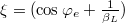 this equation has modes with frequency
  meaning that the "proper" oscillation frequency of the system in unnormalized units is

This equation shows the effect of  on the proper oscillation frequencies. Taking the limits
  or
or  in eq. (3) we see that the resulting allowed static solutions are, respectively,
  , k integer, and
  . The corresponding resonant frequencies are, respectively, the usual zero-bias Josephson plasma frequency (for all k integers) and
  .
.

Fig. 1: (a) The system subject of the present work: a superconducting loop closed by a Josephson junction; (b) example of the potential for different values of the normalized inductance of the loop but for zero applied external flux; (c) examples of the potential for an applied external flux  . It is herein assumed that the direction of the external magnetic field is always orthogonal to the plane of the loop. We can see that the effect of the applied flux is to introduce an asymmetry in the shape of the potential. The curves for the plotted potential are obtained from eq. (4).
Download figure:
Standard imageFigure 2(a) shows the frequency dependence on  around the stable equilibrium points. The plot is obtained for zero applied external magnetic flux and we can see that multiple frequencies are allowed for increasing
  . This plot has been obtained by sweeping the value of the normalized flux in the interval
 ![$[-8\pi,8\pi]$](https://content.cld.iop.org/journals/0295-5075/115/5/50004/revision1/epl18126ieqn31.gif) while finding numerically the minima of the potential (eq. (4)) for each given value
while finding numerically the minima of the potential (eq. (4)) for each given value  . The mode whose frequency tends to infinity for
  is the one of the center well of the potential while the others are those that develop for increasing values of
  in the side wells.
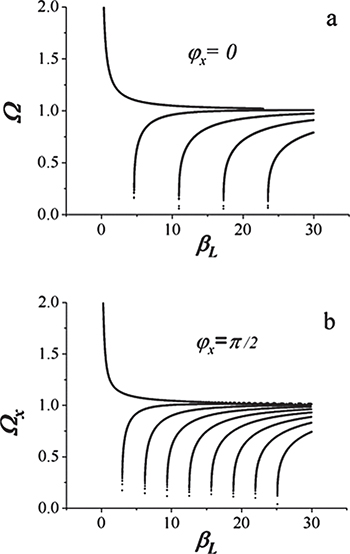
Fig. 2: Dependences of the oscillation frequencies, around the equilibrium angle, on the normalized loop inductance  for zero applied external magnetic flux (a) and for a normalized flux
  (b).
(b).
Download figure:
Standard imageLet us now turn to the non-zero applied flux case for which we apply the same analysis performed for eq. (2). That approach can be readily be applied to the non-zero flux case which will lead to the two equations

for the equilibrium angles and

for the system frequencies. Note that  becomes the previous Ω for the unbiased case, when
  . The unnormalized angular frequency
  corresponding to each
  value will be

Although eq. (11) looks formally identical to eq. (8) the external flux here introduces an asymmetry in the potential and the minima leading to values of  (eq. (9)) that are different from those of eq. (3). In fig. 2 we can see the branching of the curves of fig. 2(b) obtained for an applied external flux equal to a quarter of the flux quantum (which is
  in normalized units). The plots of fig. 2 were obtained by sweeping values of the phase in the interval
 ![$[-8\pi, 8\pi]$](https://content.cld.iop.org/journals/0295-5075/115/5/50004/revision1/epl18126ieqn41.gif) . To each of the frequency branches shown in the figures naturally corresponds a specific minimum of the potential.
. To each of the frequency branches shown in the figures naturally corresponds a specific minimum of the potential.
The spectrum of the possible frequencies as a function of the externally applied flux can be obtained from eq. (10) employing the  solutions of eq. (9) which we find numerically. In fig. 3 we see how, in the opposite plots the
  singled-value spectrum evolves in a crossing-branches spectrum for increasing values of
  . For
. For  (fig. 2(b)) and
  the resonance curves only cross at multiples of half the flux quantum (π in our normalized units) while already for
  the crossings of the branches take place for half integer values of the flux quantum. The plots of fig. 3 have been obtained by sweeping the φ values in the range
 ![$[-4\pi,4\pi]$](https://content.cld.iop.org/journals/0295-5075/115/5/50004/revision1/epl18126ieqn50.gif) . The resonant branches represent oscillation frequencies in different wells of the rf-SQUID potential.
. The resonant branches represent oscillation frequencies in different wells of the rf-SQUID potential.
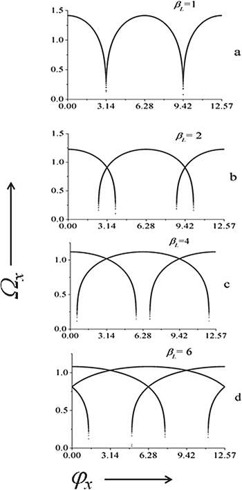
Fig. 3: The frequency spectrum of the rf-SQUID core as a function of an applied flux for different values of the normalized inductance  , indicated in the panels. We can clearly see that, for increasing values of this parameter, the system develops a number of crossing states of the resonance curves. All the crossings occur for integer and half-integer values of the flux quantum (
 in our normalized units).
Download figure:
Standard imageMore crossings for increasing values of  take place generating complex patterns. An example is given in fig. 4 for
  (a) and
  (b). We display here the results only in the field interval
 ![$[0,2\pi]$](https://content.cld.iop.org/journals/0295-5075/115/5/50004/revision1/epl18126ieqn58.gif) and, moreover in fig. 4(b) only a narrow segment of the plot along the vertical direction is presented in order to preserve clarity. At this point
and, moreover in fig. 4(b) only a narrow segment of the plot along the vertical direction is presented in order to preserve clarity. At this point  we see that three crossings take place at half the flux quantum, meaning, for example, that possible operation of the device when biased with a dc magnetic flux linking half a magnetic flux through the loop is likely going to be difficult to control in terms of frequency response. In fig. 2(b)–(d) we have only two resonant branches close to the
  point, whereas in fig. 4(a) and (b) we have, respectively, four and six resonance branches: To these resonant branches naturally one can associate different classical energy levels corresponding to given values of the external flux.

Fig. 4: Two more examples of  plots exhibiting the more complex structures that develop for increasing values of the normalized inductance of the rf-SQUID loop. In this figure, as in the others, the phase of the potential is swept in the interval
 ![$[-4\pi,4\pi]$](https://content.cld.iop.org/journals/0295-5075/115/5/50004/revision1/epl18126ieqn54.gif) .
.
Download figure:
Standard imageWe would like to emphasize that operation of the rf-SQUID core has often been considered by biasing the system with an external flux which would generate half of the flux quantum in the rf-SQUID core [9,12,13]. In this case we can see in fig. 3 and fig. 4 that the crossing of branches corresponding to different frequencies is remarkable and the resulting dynamics could be noticeably complex. For  we have two frequency crossings for
  separated roughly by a (normalized) frequency gap of 0.2, while for
  we have three crossings separated by tenths normalized frequency units. Naturally, the closer we get to integers and half-integers values of the flux quantum the smaller is the difference in frequency (and energy) between the different states corresponding to different branches. Overall we can say that the system behaves as a metaatom [6,14] with different energy states available in correspondence to given values of the applied field. These frequencies naturally represent oscillation frequencies in the wells of the potential (4).
The effect of dissipation on eq. (4) can be readily evaluated using the ansatz (5) for eq. (2). In this case we get

which tells us that, in the presence of dissipation, the angular frequency of underdamped oscillations will be

From which we see that corrections, given the values of α̣ in the experiments [10–13] typically of the order of 10−4 and below, should not be really significant.
Double-junction rf-SQUID
We now consider the two-junctions rf-SQUID system shown in fig. 5(a). Our starting point for the analysis are eqs. (7) and (8) of ref. [11]. Normalizing in these equations time and currents as we did for eq. (1) we obtain the two coupled differential equations:


The subscripts a and b for the normalized fluxes refer to the large area loop  and small area loop
  , and the two parameters
  and
and  are the normalized inductances corresponding, respectively, to the sum of the areas of the two loops and to the area of the single smaller loop;
  is the normalized inductance of a loop having area A. The factor
  accounts for an external magnetic flux applied uniformly over the two loops and
 ![$\lambda =[1+2(A/B)]^{-1} = 1/[(2\frac{\beta_{ab}}{\beta_{b}})-1]$](https://content.cld.iop.org/journals/0295-5075/115/5/50004/revision1/epl18126ieqn76.gif) is a geometrical factor since A and B are, respectively, the areas of the big loop and of the small loop in fig. 5(a) [11]. In terms of the Josephson phase differences shown in fig. 1(b)
is a geometrical factor since A and B are, respectively, the areas of the big loop and of the small loop in fig. 5(a) [11]. In terms of the Josephson phase differences shown in fig. 1(b)  and
and  we have
  and
and  .
.
Fig. 5: (a) The "double"-loop rf-SQUID system and its potential (b). The analytical form of the potential is written in eq. (22). A and B represent the areas of the two superconductive loops. Here  and
and  are spanned between
  and
and  , while the potential is spanned between −3 and 10.
Download figure:
Standard imageWe look, similarly to what we did in the previous section, for solutions of eqs. (14) and (15) in the forms


In these equations  and
and  are the equilibrium angles corresponding to solutions of (14) and (15) in the static limit. We are interested again in solutions of eqs. (14) and (15) in the form of small oscillations around equilibrium angles
  and
and  . Inserting eqs. (15) and (16) into eqs. (13) and (14), and using the small amplitudes oscillation limits
  and
and  , we obtain the two coupled equations


The two equations above are coupled damped harmonic-oscillator equations. Neglecting the loss term (an assumption which can be justified just as we did above for the single-junction case) the proper frequencies associated with eqs. (18) and (19) are

and

When looking for stable equilibrium points of the coupled system (14), (15) and (18), (19), both the conditions for the equilibrium on the two phases must be fulfilled and, therefore, in eqs. (20) and (21) the cross-cosine terms just become  in both equations. It is worth noting that the static solutions of the system of equations (1), (2) also correspond to the minima of the potential of our physical system. This potential, normalized to the Josephson energy
  , reads

This two-dimensional potential is plotted in fig. 5(b) for two  and
and  . Note that this corresponds to the case in which the areas A and B of the two loops are equal: This is not a condition that we will further investigate (we will work in the approximation
  ) but we have chosen these parameters in order to illustrate the nature of the potential and its characteristic features. It can be readily seen that setting to zero the first derivatives of the potential (22) corresponds to the static solutions of eqs. (14) and (15). We are here interested in investigating the frequency spectrum dependence of our system upon the externally applied magnetic flux
  . In order to do so we will first find, numerically, the minima of the potential function (22). These minima will provide the values of the phase to be substituted in eq. (20) and eq. (21) for determining the values of the frequencies.
In order to find the minima of the potential (22) we swept both the phases  and
and  in the interval
 ![$[-4\pi,4\pi]$](https://content.cld.iop.org/journals/0295-5075/115/5/50004/revision1/epl18126ieqn99.gif) and the externally applied flux between 0 and
and the externally applied flux between 0 and  . Setting
  and choosing a very small value for the parameter
  (10−5) we found, as expected, since the presence of the second loop is negligible, a "flux spectrum" identical to that of a single-junction rf-SQUID core having a value of the normalized inductance
  (see fig. 4(a)). This is correct since the critical current of our system is twice that of a single-junction rf-SQUID. We have then changed the values of the normalized inductances of the two loops trying to maintain our calculations close to realistic experimental parameters [12,13]. In fig. 6 we see the "flux spectrum" obtained for
  and
and  corresponding to having the area
  of the smaller loop in fig. 5(a) ten times smaller than the area
  of the larger loop. We can here see that there are now two bands of frequencies and the maximum of the upper band is 1.44 as expected from eq. (21). The upper band is just a replica, at higher frequencies, of the pattern exhibited for lower frequencies. In fig. 7(a) we show the spectrum obtained by setting
  and
and  , corresponding to the case in which the area B is 20 times smaller than A. We can clearly see that the "optical" mode moves up while the "acoustic" mode remains in the same position as in fig. 6(b). In fig. 7(b), (c) we show details of the frequency bands demonstrating that, apart from occupying a more compressed frequency interval, the two "bands" have analogous shape and branch crossing.
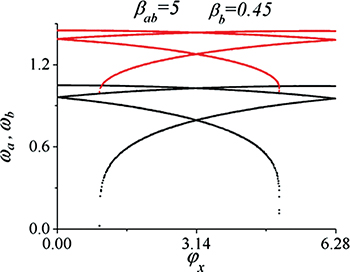
Fig. 6: The two frequency bands obtained when the inner loop area B is ten times smaller than the area A. In order to calculate the minima of the potential the phases  and
and  are swept in the interval
 ![$[-4\pi,4\pi]$](https://content.cld.iop.org/journals/0295-5075/115/5/50004/revision1/epl18126ieqn83.gif) .
.
Download figure:
Standard image
Fig. 7: (a) The frequency "spectrum" of the double squid as a function of the externally applied flux when  . The expansion of the two frequency bands is shown in (b) and (c). Here we can see the analogous shapes of the bands.
Download figure:
Standard imageWe have found the patterns of figs. 6 and 7 to be very controllable features of the spectrum of the two-junctions rf-SQUID system. This is naturally a very interesting phenomenon to consider in perspective of metadevice applications. Beside the tuning of the modes of the systems as a function of the external flux we find that an adequate choice of the ratios between the areas of the loops generates an additional (higher) band of frequency in which the system can operate. However, we have also found that attention must be paid to not letting the normalized inductance of the inner loop be close to 1. In this case we reach the point in which the single junctions of the loop could generate crossings of the modes and the resulting features become very irregular and, most likely, very difficult to control. An example of this phenomenon is shown in fig. 8 for which we have chosen  and
and  : we can see that an additional, somewhat irregular, branch appears in the frequency-vs.-flux pattern of the "optical" modes. The "acoustic" modes in this case showed the same type of pattern at lower frequencies.
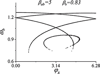
Fig. 8: An example of the somewhat irregular "branches" appearing in an optical band when the normalized inductance of the inner loop gets close to 1. In this case  .
.
Download figure:
Standard imageWe point out that several experiments have been performed independently controlling the fluxes applied to the two loops of the "double SQUID" [12,13]. Having the possibility to tune independently the fluxes means that one could perform a selection between the "acoustic" and "optical" band of operation.
Conclusions
The analysis, performed in a perturbation approach for finding the oscillation modes of rf-SQUID cores around the equilibrium angle, has shown, a variety of configurations and crossings of the branches of the different modes. The crossings of the branches occur when the external magnetic flux attains half and integer multiple values of the flux quantum. Close to these values of the external flux the response of the system to an external microwave/millimeter-wave excitation could have intriguing aspects; it is worth noting that this specific magnetic-flux bias has been often chosen for macroscopic quantum tunneling and coherence investigations [9,12]. The analysis of the case in which the junction closing the rf-SQUID loop is replaced by a double-junction interferometer has shown additional features of the system corresponding to a splitting of the response of the modes of the system in a lower ("acoustic") and a higher ("optical") frequency band. The degeneracy can be governed by adequately choosing the areas (and the inductances) of the two loops of the device. Potential applications such as those described in ref. [14] or the wide spectrum described within metamaterial research [6] open interesting perpectives for the future of a system which has already substantially contributed to the development of the research in fundamental and applied superconductivity.
As far as microwave and millimeter-wave fields reaching the rf-SQUID region are concerned, one can reasonably assume that the radiation fields will be distributed uniformly in the loop areas and in the junctions; however, we should bear in mind that the magnetic fields in the two loops of the double-loop rf-SQUID can be controlled independently [12,13]. This means that the two modes, the acoustic mode and the optical one, can be tuned independently and this represents another interesting direction for future devices. From the "rf" point of view, however, the relevant feature of the system having two frequency bands remains unchanged. High-frequency features of the Josephson junctions have demonstrated, over the years, that this field is very rich and intriguing and there still are features which have not been explained [15]. We have herein provided evidence, through a systematic analysis, that a basic superconducting system could lead to further experimental rf work and devices.
Throughout the paper we have normalized time to the inverse of zero-bias Josephson plasma angular frequency  . This is a very well-known parameter in Josephson research and, for current densities in the range (100–1 kA) A/cm2 it attains values in the interval (0.4–1.3) × 1012 rad/s meaning that the frequencies will be roughly in the range 60–200 GHz. Here we have considered a standard trilayer Nb-NbAlOx-Nb fabrication process for which the specific capacitance of the junctions is of the order of 0.05 F/m2 [15]. From these estimates it follows that we investigated issues in a range of the electromagnetic spectrum which is still of noticeable interest for applications. An "optical" mode of the double rf-SQUID that we analyzed could have proper frequencies around 300 GHz.