


Abstract
We study the impact of the interaction of nodes in a layer of a multiplex network on the dynamical behavior and cluster synchronization of these nodes in the other layers. We find that nodes interactions in one layer affect the cluster synchronizability of the other layer in many different ways. While the multiplexing of a sparse network with the other sparse networks enhances the cluster synchronizability of the individual layer, multiplexing with dense networks suppresses the cluster synchronizability with the network architecture deciding the impact of the enhancement and the suppression. Additionally, at weak couplings the enhancement in the cluster synchronizability, due to multiplexing, remains of the driven type, while for strong couplings the multiplexing may lead to a transition to the self-organized mechanism. The results presented here have applicability in regulating the synchronizability of a particular layer of real-world systems having multiplex architecture.
Export citation and abstract BibTeX RIS
Introduction
Synchronization is a universal phenomenon observed in a range of systems [1]. It is known to be important for the proper functioning of many complex systems. For example in the brain, the phase synchronization at different locations is responsible for action, motion, vision and sensation [2]. Recently, cluster synchronization has gained tremendous attention due to its occurrence and importance in many real-world systems [3–5]. The cluster synchronization refers to the case when the nodes of a system divide into several synchronized groups such that nodes in the same group synchronize with each other while do not synchronize with the nodes of the other groups. So far the studies on the cluster synchronization have mainly focused on complex systems being represented as isolated networks [6–8].
However, a complex system may consist of a superposition of a number of interacting networks [9,10], such as a social system which is composed of different sub-networks consisting of family, friends, colleagues, work collaborators and hence forming a multiplex network. The realization that multiplex networks present a more realistic representation of real-world interactions, has led to a spurt in the activities of modeling real-world complex systems [9,11–13] under this framework.
Most of the studies on multiplex networks have concentrated on the investigation of various structural properties or on the emergence of spectral properties [14,15]. Few works considering dynamical properties report that multiplexing reduces the rate of the global synchronization and may lead to an explosive synchronization [16]. Though, such understanding for the cluster synchronization of the multiplex networks is lacking.
In this letter, we investigate the dynamical behavior of nodes in a layer upon multiplexing it with another layer. Particularly, we investigate the impact of nodes interactions in one layer on the cluster synchronization of the same nodes in the other layer.
In a realistic situation, the connection density as well as the network architecture of two layers can be different, for instance in a social system a family network can be denser than a counter friendship network as well as can have a different network architecture. Similarly, the friendship network can be denser than a corresponding business network. In this work we consider model networks studied widely which are known to capture many properties of the real-world systems, for instance of social networks. One of the most important property captured by the scale-free (SF) network is the power law degree distribution of many social networks.
We find that nodes interactions in one layer affect the synchronizability of the other layer in many different ways. While multiplexing with sparse networks enhances the cluster synchronizability of a layer, the impact of multiplexing with dense networks depend on the network architecture. The enhancement in the cluster synchronization is referred to the case when the number of the nodes forming synchronized clusters increases. Furthermore, we report that the change in the density of connections in a layer of the multiplex network may bring a change in the mechanism of the cluster synchronization in the other layer. Previous studies on the dynamical behavior of isolated networks have identified two different mechanisms of cluster synchronization, namely, the driven (D) and the self-organized (SO) [4]. The D and SO synchronization correspond to the synchronization due to the inter- and intra-cluster couplings, respectively.
We consider the well-known coupled maps model [17] to investigate the phase-synchronized clusters in the multiplex networks. Furthermore, we consider phase synchronization instead of the exact synchronization ( and t > t0) as for sparse networks number of nodes displaying the exact synchronization is very less and with an increase in the connection density there is a transition to the globally synchronized state spanning all the nodes [9], whereas the prime motive of the current work is to study the cluster synchronization. The phase synchronization reveals interesting cluster patterns as well as the dependence of the mechanism of cluster formation in one layer on the network structure of the other layers. Let each node of the network be assigned a dynamical variable
  . The dynamical evolution is defined by
Here, A is the adjacency matrix with elements Aij taking values 1 and 0 depending upon whether there is a connection between i and j or not, ε is the overall coupling constant, N is total number of nodes in a layer and m is the number of layers in the multiplex network. We consider the simplest multiplex network with two layers and N nodes in each layer (fig. 1), the adjacency matrix A for this two-layer multiplex network can be given as
where, A1 and A2 are the adjacency matrices corresponding to the layer 1 and layer 2.  is the degree of the i-th node in the l-th layer of the multiplex network.
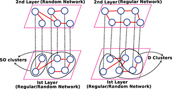
Fig. 1: (Color online) Schematic diagram depicting a multiplex network with two layers. The dashed lines indicate the inter-layer connections. The density of connections in the different layers can be different and is defined as  for the first layer and
  for the second layer.
Download figure:
Standard imageThe average degree of the two layers may be different and is indicated as  and
and  . The function f(x) defines a local nonlinear map, whereas g(x) defines the nature of coupling between the nodes. The local nonlinear map f(x) is considered as the logistic map (
 ,
,  ) and the coupling function is taken as
  .
.
We consider phase synchronization defined as follows [4,18]. Let ni and nj denote the number of times when the variables  and
and  ,
,  for the nodes i and j exhibit local minima (maxima) during the time interval T. Let nij denote the number of times these local minima (maxima) match with each other. The phase distance between two nodes i and j is then given as
  . The nodes i and j are phase synchronized if
  . All the pairs of nodes in a cluster are phase synchronized1
. Further, we define cluster synchronizability of a network in terms of the number of nodes participating in the clusters. In order to measure the cluster synchronizability, we define the measure
. All the pairs of nodes in a cluster are phase synchronized1
. Further, we define cluster synchronizability of a network in terms of the number of nodes participating in the clusters. In order to measure the cluster synchronizability, we define the measure  , where
  is the total number of nodes participating in all the clusters. A network exhibits better synchronizability if
  of this is more than the
  of another network in a larger range of coupling.
Furthermore, to investigate the mechanism behind the cluster formation, we use  and
and  as a measure for the intra- and inter-cluster couplings, respectively [4], which are defined as;
  and
and  . where
  and
and  are the numbers of intra-cluster and inter-cluster couplings, respectively. In
  , couplings between two isolated nodes are not included. The ideal D cluster state corresponds to
  , whereas for the ideal SO cluster state
  can take a very small value but cannot attain the zero value as at least there is one connection between different clusters for a connected network. Note that, while calculating the values of
  and
and  for a particular layer, we do not consider the inter-layer connections. Further, if
  , clusters are considered here to be of the dominant SO (dominant D) type.
We study the impact of multiplexing on the cluster synchronizability of the random as well as the regular networks. The 1-d lattices used in the simulation have circular boundary conditions with each node having k nearest neighbors. The scale-free (SF) and random networks are obtained by using BA and ER models, respectively [19]. This letter focuses on the cluster synchronizability of networks and hence we consider sparse networks representing the first layer as denser networks that tend to form the global synchronized state spanning all the nodes.
We evolve eq. (1) starting from a set of random initial conditions and consider the phase-synchronized clusters after an initial transient. For the two-layers multiplex network, the first layer can be represented by a regular or a random network, similarly the second layer can also be represented by a regular or random network. Here, we present results for all the possible combinations, such as random-random, random-regular, regular-regular and regular-random. First, we discuss the cluster synchronizability of a regular network represented by a 1-d lattice upon multiplexing with a ER random network. The isolated sparse 1-d lattice at weak couplings leads to the phase-synchronized clusters with all the nodes participating in the clusters, whereas strong couplings lead to a very few nodes forming clusters (fig. 2(a)). The multiplexing with a sparse ER network enhances the cluster synchronizability of the 1-d lattice at all the couplings as well as maintains the good cluster synchronizability exhibited by the isolated networks at the weak coupling range  . The multiplexing with a denser ER network while enhances the cluster synchronizability of 1-d lattice at weak couplings, it leaves the cluster synchronizability unchanged with few nodes keep forming synchronized clusters at intermediate and strong couplings. For example, fig. 2(b) demonstrates that cluster synchronizability of 1-d lattice enhances at weak couplings irrespective of the value of
  , whereas at the intermediate couplings, for
  , there is an enhancement in the cluster synchronization, which for the higher values of
  gets vanished.
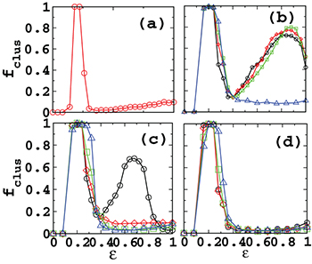
Fig. 2: (Color online) Variation of  with respect to ε for (a) an isolated 1-d lattice and for the 1-d lattice
  multiplexed with (b) ER random networks, (c) SF networks and (d) 1-d lattice of different average degree
  . The solid lines with open circle, diamond, square and triangle correspond to
  , and 20 respectively. The average degree of the first layer remains the same for all three cases. For all the layers
  and diagrams are plotted for an average over 20 random realizations of the networks and 40 initial conditions.
Download figure:
Standard imageAt strong couplings, the cluster synchronization enhances up to a certain value of  as depicted in fig. 2(b). For a 1-d lattice of
  and
and  , synchronization enhances up to
  (fig. 2(b)). The denser connections in the second layer do not enhance the cluster synchronizability of the first layer with sparser connections. Note that the synchronizability of the second layer, represented as the ER random network, increases with an increase in the average degree as observed for the isolated networks.
Next we discuss the cluster synchronizability of the 1-d lattice upon multiplexing with various other network architectures. At weak couplings, multiplexing with the SF networks also leads to an enhancement in the cluster synchronizability (fig. 2(c)), as observed for the multiplexing with the ER random network. Whereas at intermediate and strong couplings, there is an enhancement in the cluster synchronizability as observed for the multiplexing with the random networks, but the connection density of the second layer for which this enhancement occurs becomes lower (fig. 2(b)). For example, a 1-d lattice with  , exhibits an enhancement in the cluster synchronization upon multiplexing with the SF networks of
  (fig. 2(c)).
The multiplexing of the 1-d lattice with another 1-d lattice does not enhance the cluster synchronizability of the 1-d lattice at intermediate and strong couplings (fig. 2(d)). Thus, the enhancement in the cluster synchronizability of the 1-d lattice is least favorable when it is multiplexed with the 1-d lattice and most favorable for multiplexing with the ER random networks. A very high diameter of the 1-d lattice has been attributed for its poor synchronizability [20,21]. Multiplexing of the 1-d lattice with the other 1-d lattice keeps the diameter of the network almost same as for the isolated network, whereas multiplexing with the random networks leads to a sharp reduction in the diameter of the entire network as well as of the layer represented with the 1-d lattice as any pair of the distant nodes get connected with a shorter path via the layer represented by the ER random network. For example, the diameter of the 1-d lattice with N = 250 and  is 63. Upon multiplexing with the other 1-d lattice (N = 250,
  ) the diameter becomes 64. Hence, the synchronizability remains unaffected after the multiplexing. While multiplexing with the ER random network of the same average degree, the diameter of the entire multiplex network reduces to 8.
Further, we investigate the cluster synchronizability of the ER random networks upon multiplexing with a various network architecture. The isolated sparse ER random networks demonstrates a better cluster synchronizability as compared to the sparse regular networks (fig. 3(a)). First, we discuss the impact on the cluster synchronizability of ER random networks upon the multiplexing with the 1-d lattice. At weak couplings, the multiplexing with a 1-d lattice as well with other ER random network enhances the cluster synchronization of the ER network. The enhancement is higher for the multiplexing with the ER random network. For example, the isolated ER random networks with  and
and  lead to the participation of about 50% nodes in the cluster formation. After multiplexing with the 1-d lattice, 65% nodes keep participating in the cluster formation as shown in fig. 3(b), whereas multiplexing with the ER random networks leads to the participation of 80% nodes in the cluster formation (fig. 3(c)). The range of coupling in which enhancement occurs keeps on increasing with the increase in the density of the second layer (fig. 3(b), (c)). At intermediate and strong couplings, there is an enhancement in the synchronization for multiplexing with the sparse networks whereas the impact of multiplexing with the dense networks largely depends on the network architecture as we discussed for the 1-d lattice. For example, the cluster synchronizability of ER random networks with
  enhances upon multiplexing with the 1-d lattice and ER random networks up to a certain limit of
  . The multiplexing with the 1-d lattice enhances the cluster synchronizability for
  (fig. 3(b)), while in the case of multiplexing with the ER random networks the enhancement occurs for
  (fig. 3(c)). The higher connection density in the second layer leads to the suppression in the cluster synchronizability of random networks (fig. 3(a), (b) and (c)). Infact multiplexing of the sparse ER random network with the globally connected network also leads to a suppression in the cluster synchronizability of the random network, as well as it destroys the global synchrony in the globally connected layer. Note that as a layer becomes denser, it shows an enhancement in the cluster synchronizability, but there is a reduction in the cluster synchronization as compared to the corresponding isolated networks. Thus, the cluster synchronizability of the first layer mainly depends on its own network architecture and on the network architecture of the second layer.

Fig. 3: (Color online) Variation of  as a function of ε for (a) an isolated ER random network and for the ER random network
  multiplexed with (b) 1-d lattices and (c) ER random networks of different average degree
  . The solid lines with open circles, diamonds, squares, up and down triangles correspond to
  and 80, respectively. The average degree of the first layer remains the same for all the three cases. For all the layers
  and diagrams are plotted for an average over 20 random realizations of the networks and 40 initial conditions.
Download figure:
Standard imageIn order to demonstrate the generality of the enhancement in the cluster synchronizability of a sparse network upon multiplexing with the other sparse network, we present values of  with error bars in fig. 4. It reflects a clear enhancement in the cluster synchronization after multiplexing.
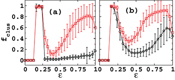
Fig. 4: (Color online) Variation of  as a function of ε for (a) 1-d lattice and (b) ER random networks. Symbols ∘ and □ represent
  before and after multiplexing, respectively. The average degree of both the layers remains the same
  . For all the layers
  , and diagrams are plotted for an average over 20 random realizations of the networks and 40 random realizations of the initial conditions.
Download figure:
Standard imageFurther, in order to understand the suppression in the cluster synchronizability of a sparse network upon multiplexing with the denser networks, we examine the degree-degree correlation of the mirror nodes. We calculate the Pearson coefficient for the degree-degree correlation of the mirror nodes, given as follows [22]:  , where ejk is the fraction of the j-degree node connected with k-degree nodes. qj is the fraction of all the nodes connected to the j-th degree, yielding
  ,
,  . Figure 5(a) plotting the variation of r with
  demonstrates that the multiplexing of a sparse network with a denser network corresponds to the strong disassortivity [22] in the degree-degree correlations of the mirror nodes. For r > 0.85, irrespective of the network architecture, the cluster synchronizability of the sparse network is suppressed, while the denser network loses the global synchrony, which is indicated in the isolated case at the strong couplings. Thus, the strong disassortivity in the degree of the mirror nodes is associated with the suppression in the synchronizability of both the networks. Additionally, the multiplex network yields the chaotic dynamics for almost all the coupling values for the layers being represented by sparse networks (fig. 5(b)).
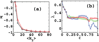
Fig. 5: (Color online) (a) The largest Lyapunov exponent for a multiplex network consisting of two layers, one represented by the ER random  network and the other by the 1-d lattice for various average degree
  . Symbols ∘, ◊, and ▵ correspond to
  and 6, respectively. The number of nodes in each layer is N = 100. (b) Variation of the Pearson correlation coefficient r for 1-d lattice-ER
  and ER-ER
  multiplex networks as a function of
  . The average degree of the first layer (
 and N = 250) remains the same in each layer.
Download figure:
Standard imageThe network parameters for which the multiplexing imposes a change in the dynamical behavior may change with an increase in the network size but the observation that there is an enhancement in the synchronization of a sparse network upon multiplexing with the other sparse networks, and the suppression due to the multiplexing with the dense networks remain the same. For example, the limit of  , for which there is an enhancement in the synchronization at strong couplings, depends on the network properties such as the average degree and the size of the network. For the 1-d lattice of N = 100 and
  the enhancement occurs for
  (fig. 6(a)) upon multiplexing with the random network, while for the random network with
  and
and  , an enhancement in the synchronization occurs up to
  (fig. 6(b)) upon multiplexing. Furthermore, the fraction of the nodes in the largest cluster
  also exhbits an enhancement in cluster synchronization upon multiplexing with the sparse networks (fig. 6(a) and (b)) and a suppression upon the multiplexing with the denser networks (fig. 6(b)).
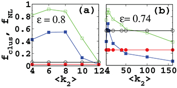
Fig. 6: (Color online) Variation of  and fNL (size of the largest cluster divided by the network size) as a function of
  for a 1-d lattice and a random network of various network sizes. Open symbols □ and ∘ correspond to the values of
  for the first layer, before and after its multiplexing, respectively. Closed □ and ∘ correspond to fNL for the first layer, before and after multiplexing, respectively. (a) 1-d lattice of N = 100,
  before and after its multiplexing with the random network. (b) Random network of N = 500,
  before and after its multiplexing with the 1-d lattice. The coupling values at which the enhancement in the cluster synchronization followed by a suppression at the strong coupling is observed may change with the network size and the architecture but the phenomenon remains valid for the sparser networks. All the graphs are plotted for an average over 10 different realizations of the networks and 20 random realizations of the initial conditions.
Download figure:
Standard imageFurther, we investigate the mechanism behind the cluster formation in multiplex networks. We find that at weak couplings, the enhancement in the cluster synchronizability due to multiplexing, corresponds to an enhancement in the D mechanism indicating that the D synchronization remains the prime mechanism behind the cluster formation even after multiplexing, as observed for the isolated networks [4]. For example, the cluster synchronizability of a 1-d lattice of N = 50 and  is enhanced due to the multiplexing with ER random networks of
  and clusters are of dominant D type (fig. 7(a), (b)). At intermediate and strong couplings, the multiplexing may lead to a change in the mechanism behind the cluster formation. The 1-d lattice, which manifests a very poor cluster synchronizability at intermediate and strong couplings, upon multiplexing exhibits an enhanced cluster synchronizability with the dominant SO mechanism. For example, the 1-d lattice of N = 50 and
  does not indicate any significant cluster formation at strong couplings (fig. 7(c)). After multiplexing with the ER random network
  , the 1-d lattice starts displaying the dominant SO clusters (fig. 7(d)). The isolated random as well as SF sparse networks exhibit a transition from the ideal D or mixed cluster state to the dominant SO cluster state. For example, the random network of N = 50 and
  exhibits a transition from the mixed cluster state (fig. 7(e)) to the dominant SO cluster state (fig. 7(f)) and the SF network shows a transition from the mixed and the dominant D cluster state to the dominant SO cluster state (fig. 8(a) and (b)) upon its multiplexing with the 1-d lattice. Moreover, note that multiplexing of the sparse networks with the dense networks leads to a suppression in the cluster synchronization at strong couplings, which also corresponds to the suppression in the SO mechanism, while the contribution of the D mechanism remains the same as observed for the isolated network (fig. 8(a), (b)).
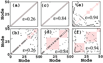
Fig. 7: (Color online) Node vs. node diagram, before and after the multiplexing for various different combinations of the networks. (a), (c) represent an isolated 1-d lattice and (b), (d) represent 1-d lattice after multiplexing with the ER random network of  . (e) Isolated random network of
  and (f) after its multiplexing with the 1-d lattice of
  . Open circles
  represent the synchronized clusters and the closed circles
  represent connections. Large square blocks indicate that all the nodes in a particular block are phase synchronized forming a cluster. For all the panels N = 50 in each of the layers. Node numbers are reorganized such that those belonging to the same cluster come consecutively.
Download figure:
Standard image
Fig. 8: (Color online) Variation of  and
and  as a function of
  for an SF network. Symbols ◊ and □ correspond to
  and
and  , respectively, for isolated SF networks, whereas symbols ∘ and ▵ correspond to the values of
  and
and  , respectively, for the first layer (SF networks) after its multiplexing with the ER random networks. For all the networks N = 250 and
  . All the graphs are plotted for an average over 10 different realizations of the networks and 20 random realizations of the initial conditions.
Download figure:
Standard imageTo conclude, we have studied the impact of multiplexing on the cluster synchronizability as well as the mechanism behind the synchronization of a layer represented by the sparse networks in the simplest multiplex network consisting of two layers. We find that at weak couplings, the multiplexing enhances the cluster synchronizability, while at strong couplings this enhancement depends on the architecture as well as the connection density of the other layer. The cluster synchronizability of a layer is enhanced when the other layer has a moderate connection density. Moreover, multiplexing favors the enhancement in the cluster synchronization of a regular network if it is multiplexed with another random network. The enhancement in the cluster synchronization is also associated with the change in the mechanism of the cluster formation.
Our work demonstrates that in a multiplex network, the activity in one layer (sub-network) is significantly influenced by the structural properties of the other layer (sub-network). If the connection density in one layer increases above a certain limit, it may spoil the synchronization in the other layer. The results presented here about the dynamical behavior of multiplex networks may provide a guidance for the construction of a better model network with multiplex architecture, such as the airport networks composing different airline companies [23]. Furthermore, as the largest eigenvalue of the adjacency matrix defines the threshold of the epidemic spread [24] as well as the global synchronizability [25] of a network, suppression in the synchronizability of the denser networks, upon multiplexing, can be used to control epidemic spread [14] by introducing a different kind of relation among the same set of nodes, for instance establishing some health awareness camp [26], which can act as the other layer consisting of connections between the nodes which are the participants of that camp.
Acknowledgments
SJ acknowledges DST (EMR/2014/000368) and CSIR (25(0205)/12/EMR-II) project grants for the financial support. AS thanks complex systems lab members for useful discussions.
Footnotes
- 1
Note that the definition of phase synchronization used here assign antiphase-synchronized nodes into two different clusters due to phase distance being one. However, this particular situation of nodes being antiphase synchronized is not so often observed for the chaotic evolution.