

Abstract
The growing amount of carbon dioxide in the atmosphere is often considered as the dominant factor for the global warming during the past decades. The noted correlation, however, does not answer the question about causality. In addition, the reported temperature data do not display a simple relationship between the monotonic concentration increase from 1880 to 2010 and the non-monotonic temperature rise during the same period. We have performed new measurements for optically thick samples of CO2 and investigate its role for the greenhouse effect on the basis of these spectroscopic data. Using simplified global models the warming of the surface is computed and a relatively modest effect is found, only: from the reported CO2 concentration rise in the atmosphere from 290 to 385 ppmv in 1880 to 2010 we derive a direct temperature rise of  . Including the simultaneous feedback effect of atmospheric water we still arrive at a minor CO2 contribution of less than 33% to the reported global warming of
  . It is suggested that other factors that are known to influence the greenhouse effect, e.g. air pollution by black carbon should be considered in more detail to fully understand the global temperature change.
Export citation and abstract BibTeX RIS
Introduction
Analysis of isotope and gas concentrations of the antarctic ice-core provides important information on the atmospheric composition and climate variations in the past four glacial-interglacial cycles [1–3]. The data show correlation between surface temperature and carbon dioxide (and methane) concentration. The role of CO2 in these changes however remains unclear since the temperature increase seems to precede the CO2 growth [1]. Taking into account the large amount of CO2 dissolved in the sea and its declining solubility for higher temperatures it was suggested that the CO2 rise is a result and amplifier of the global warming rather than its cause [4,5]. However, a recent study over 80 proxy records reports that temperature generally lags CO2 during the last deglaciation [6].
Of particular interest is the global warming observed in the last 130 years since it could have anthropogenic reasons [7–11]. Sophisticated computer simulations were reported that estimate the impact of the growing concentrations of greenhouse gases and predict a further temperature rise of 1 to 6 K during the present century [12–18]. In addition, analyses of black carbon and tropospheric ozone reveal that other anthropogenic pollutants contribute notably to the observed temperature rise and changes of major climate zones [19,20]. It has been also suggested that periodic variations in the solar activity are the main cause for global temperature changes during the past 130 years [21]. But in spite of the close correlation observed between sunspot activity and variation of terrestrial temperature, the changes of the solar irradiation of  [22] seem to be too small compared to the measured global warming. Other authors report a close correlation between cosmic rays, ozone depletion and concentration of halocarbons in the atmosphere [23]. These observations give evidence that global warming in the last 60 years was possibly caused by the significant increase of chlorofluorocarbons. Calculations of the greenhouse effect of halocarbons on the other hand predicted a global cooling for the next five to seven decades [24]. Obviously the role of the greenhouse gases should be re-investigated on the basis of additional experimental data.
In combination with atmospheric water, CO2 and the other greenhouse gases display a broad-band absorption of the thermal emission of the terrestrial surface, with the exception of several spectral windows. The latter fact is illustrated by the satellite measurements in fig. 1(a), taken from literature [25,26]. The far-infrared emission of the earth is plotted vs. frequency in units of wave numbers. The transmitted radiation through the atmospheric window from approximately 750 to  is readily seen, limited on the low-frequency side by the
  -absorption of CO2 and by an ozone band at higher frequencies [27]. Around the
  -band center at
  [28] the surface emission is totally absorbed. However, carbon dioxide in turn gives rise to thermal radiation that is weaker because of the lower temperature of the atmosphere [29]. A second window is indicated in fig. 1(a) above
  between the ozone feature and a water band [27].

Fig. 1: (a) Satellite observation of the thermal emissions of the terrestrial surface and atmosphere; black measured line [26]; the colour curves are calculated for a black radiator with the respective temperature indicated. (b) Schematic of the thermal radiation of the surface represented by a black radiator with  (black and red solid line); absorbed spectral intervals are indicated by the coloured areas for water, ozone and CO2; spectral windows of the atmosphere in white. The nonlinear ordinate and abscissa scales of (b) should be noted.
Download figure:
Standard imageIn fig. 1(b), a schematic picture of the spectroscopic situation is presented in a larger spectral range including the  -band of CO2 centered at
  [28]. The terrestrial surface with an assumed temperature
  [7] is treated as a black radiator following Planck's law (solid curve) [29]. The spectral intensity per frequency unit is plotted vs. frequency. The nonlinear ordinate and abscissa scales of fig. 1(b) should be noted that were chosen for a better display of the details. For the assumed temperature the maximum surface emission occurs at
  close to the position of the
  -band and drops rapidly for larger wave numbers, e.g. by a factor of
  at
at  . The absorption regions of CO2 and water of our model atmosphere are indicated by red and blue regions, respectively. The narrow ozone band is depicted in violet. Further contributions are buried in the strong water bands and/or have a small effect. The transmission of the atmosphere in several spectral windows, labelled (1) to (3), is readily seen. There is overlap between the low-frequency wings of the
  and
and  bands of CO2 and adjacent water bands so that the extensions of the respective red wings of the former are not relevant. The absorption bands of methane around 1300 and
  [28,30] are buried in the strong water bands and omitted in the figure. We also mention its small concentration of
  . For nitrous oxide with even smaller concentration of 0.3 ppmv the situation is similar with absorption bands around 589, 1285 and
  [30]. CH4 and N2O are neglected in our model atmosphere that is also considered in our computations discussed below. Thermal reemissions of the greenhouse gases are not indicated in fig. 1(b).
The present work is restricted to a discussion of the global warming as revealed by reliable empirical data. Only the role of CO2 will be discussed relating new spectroscopic data with 1-dimensional global models and using some recent empirical results. We confine ourselves to a simplified physical picture of the greenhouse effect so that only semi-quantitative results can be expected.
Experimental
We have obtained precise data on the transmission of optically dense CO2 samples in the wave number range  . Our experimental system was a Tensor 27 Fourier-transform infrared spectrometer (FTIR, Bruker Optics) with a spectral resolution of
  . The sample cell was 10 cm long with KBr windows. To remove impurities, the sample was filled and evacuated several times with high purity CO2 (99.995%). The pressure was kept at 2 bar for measurements in the temperature range 220–295 K. The temperature was controlled by a cryostat and directly measured in the sample. An overview spectrum is presented in fig. 2(a). The wings of the
  -band at
  are extended by various hot bands [28] included in our computations. The situation is similar for the
  -band with the low-frequency wing extended by the corresponding mode of 13C16O2 at
  [28]. For the concentration range of interest
  and the thickness of the atmosphere we estimate the optical density
  in the band center of
  to be
to be  (for
(for  :
:  ). In other words there is total absorption around the band centers not depending on concentration changes. Thus only the wings of the
  and
and  absorptions are relevant for concentration changes of CO2, indicated in the figure by red circles. The relatively weak absorption by hot bands at 791, 961 and
  are also important because they modify the spectral windows of the greenhouse effect and were carefully measured.
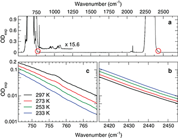
Fig. 2: (a) Overview infrared absorption spectrum of neat CO2 at a pressure of 2.0 bar and temperature of 297 K; sample length 10 cm. The relevant hot bands are depicted with a magnification factor of 15.6. (b) and (c): OD of the sample of (a) at various temperatures (see the legend) in the interesting regions.
Download figure:
Standard imageSome experimental results on the temperature dependence of the CO2 absorption bands are presented in figs. 2(b) and (c). The measured  of the high-frequency wings is plotted on a logarithmic scale vs. wave number. For atmospheric conditions, the experimental OD-values of the ordinate scales have to be multiplied by a factor of approximately 15.6. The measured OD of the sample was converted to the situation in the atmosphere using Beer's law and the barometric formula for an effective thickness of the atmosphere of 7990 m. The concentration dependences of the wings are readily deduced from our data. A concentration rise of 33% (290 to 385 ppmv) [31] in the atmosphere with mean temperature 255 K increases the effective
  -width by
  (relative broadening 2.3% of the band). The effective width is defined here as the halfwidth at 50% band transmission (HWHM). The corresponding number for the
  -band is
  (relative broadening 5.5%).
Theoretical models
For computations of the greenhouse effect we introduce the integrated absorptivity η of the atmosphere for the infrared emission of the surface. Due to the spectral windows only a fraction  is absorbed by the atmosphere while the remaining part
  of the surface emission is transmitted into the universe. The quantity depends on concentration (molar fraction x, in units of ppmv) and the mean temperature Tat of the absorbing CO2 molecules,
  , and is evaluated from our spectroscopic data. The other greenhouse gases are assumed to be constant. The surface temperature Ts comes in since the spectral intensity distribution of the surface emission is temperature-dependent (compare with Wien's law) [29]. For the approximate global values
  and
and  [7] and using the effective bandwidth changes mentioned above we estimate an increase of the efficiency of
  for the concentration change from 290 to 385 ppmv.
As extension of the well-known 2-layer model for the greenhouse effect [32,33] we have developed models where the atmosphere is arbitrarily divided into two and more parts with respective temperatures Ti. In this way the temperature variation of the atmosphere is included. The spectral efficiencies  of the layers have to be distinguished. Transport phenomena between the layers are included by additional parameters but are found to have little quantitative effect on the global surface warming by CO2. The efficiencies
  are computed from our spectroscopic data, the temperatures Ti being self-consistently determined from thermal equilibrium. Radiative equilibrium is considered between the solar input, and the thermal emissions of the surface and the various layers of the atmosphere. In spite of the simplicity of our models the results are believed to be significant, since the global properties of the earth have to be consistent with energy conservation arguments explicitly treated by the models. The use of a 1-dimensional model is fully justified if the CO2 concentration dependences of the geographic and seasonal variations of the surface temperature need to be expanded to first order, only. The problem is thus linearized and a global average over geographic and seasonal changes can be carried out first before evaluating the mean concentration-induced temperature rise, i.e. the 1-dimensional treatment is sufficient. The first order approach is believed to be an acceptable approximation because of the moderate concentration increase of
  of CO2 and the small rise of the mean surface temperature.
The level scheme in the case of a 4-level model is shown in fig. 3. Assuming equal absorption of the three atmospheric parts the thickness of the layers is estimated from the barometric formula to be 3.2 and 5.6 km (layer 1 and 2, respectively), while the top layer extends above 8.8 km into the universe. The spectral efficiencies  are calculated from the measured absorption properties of CO2 without a fitting parameter. The surface (0) with temperature Ts is treated as a black radiator with intensity
  (spectral efficiency of 1, Stefan-Boltzmann constant σ). The atmospheric layers are treated as selective emitters with temperatures Ti,
  . Quasi-equilibrium between the intensity input and output of the individual layers leads to the following equations:


Here  denotes the spectral efficiency by absorption of layer j, while subscript i labels the origin of the thermal radiation. The parameters are evaluated from the measured OD-values by integration over the spectrum without a fitting parameter. Details will be described elsewhere. A numerical solution of the above equations delivers the temperatures of the 4-layer model of, respectively, 231 K, 261 K and 277 K for the upper, middle and lower part of the troposphere, while the surface temperature is taken to be
  (for
(for  in 1880). The specific parameter values of Ai and Bi determine the temperatures of layers (1) to (3) but have little influence on the CO2 concentration effect of the surface temperature as shown by the data of tables 1 and 2.
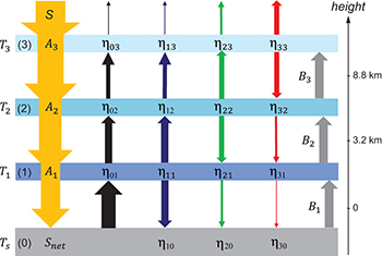
Fig. 3: 4-level model for the greenhouse effect with the surface (0) and atmospheric layers (1)–(3). The solar input (total value S) is indicated by yellow arrows with parameters  (surface) and
  (atmosphere,
  ). The thermal emission of the layers is illustrated by arrows. The heat transport by non-radiative mechanisms is represented by grey arrows (parameters Bi). The
  denote the spectral efficiencies of the respective layers j.
Download figure:
Standard imageTable 1:.
CO2 concentration effect on the layer temperatures from 1880 to 2010 keeping the surface temperature in 1880 constant at 288.0 K. The direct solar input into the atmospheric layers  is varied. The resulting surface temperature change
  is approximately constant.
| Ain (W/m2) |  / /  % % |
 (mK) (mK) |
 / /  / /  (mK) (mK) |
|---|---|---|---|
| 53.51 | 10 / 20 | 254 | 165 / 101 / 44 |
| 63.43 | 20 / 40 | 262 | 146 / 72 / 34 |
| 67.42 | 30 / 33 | 261 | 137 / 70 / 34 |
| 84.87 | 45 / 45 | 268 | 101 / 29 / 20 |
| 99.91 | 70 / 20 | 268 | 69 / 22 / 13 |
Table 2:.
The same as table 1 varying the input parameters  describing the heat transport from the surface to the atmospheric layers. The small effect on
  is noteworthy.
| Ain (W/m2) | B1 / B2 / B3 (W/m2) |  (mK) (mK) |
 / /  / /  (mK) (mK) |
|---|---|---|---|
| 100.47 | 10 / 8 / 4 | 268 | 111 / 37 / 23 |
| 84.52 | 25 / 20 / 10 | 267 | 113 / 38 / 24 |
| 76.33 | 30 / 30 / 12 | 267 | 120 / 38 / 25 |
| 73.36 | 30 / 30 / 18 | 265 | 125 / 49 / 28 |
| 29.98 | 70 / 70 / 28 | 267 | 134 / 39 / 27 |
The quantities  (total solar input), albedo
 and the surface temperature
  are kept constant as empirical facts. The direct solar input Ain into the atmosphere is adjusted correspondingly to maintain this temperature. With respect to previous results a range of 50 to
  is considered (see column 1 in the tables). Column 2 of table 1 with
  values indicates how the input Ain is distributed over the atmospheric parts
  . The numbers 30 and 33% (so that
  ) refer to the situation where the solar energy deposition into the three layers is approximately equal. The corresponding temperature increase
  of the surface for a CO2 concentration rise from 290.4 (in 1880) to 385 ppmv in 2010 (see below) is listed in column 3. It is important to note that the numbers are approximately constant within a few mK. The column 4 states the computed CO2-induced temperature rise of the atmosphere with small variations of
  in spite of the considerable change of the solar input parameter.
The effect of parameters Bi describing the heat transport is addressed by table 2 (see column 2). Quite obviously varying the energy loss of the surface (parameter B1) requires a compensation by a similar change of Ain in column 1. The third column again shows that the computed concentration effect for 1880 to 2010 on the surface temperature is remarkably insensitive to the differing input parameters with  . Column 4 again indicates the concentration effect on the layers with variations of
  below 100 mK. The corresponding temperature values T1 to T3 of the atmosphere in tables 1 and 2 for
  cover ranges of 273–284 K (1), 254–269 K (2) and 230.5–230.9 K (3), respectively.
Results and discussion
We now discuss the causal relationship between CO2 concentration and global surface temperature. We recall that an empirical correlation does not answer the question what factor determines the other one. The situation is illustrated by the reported data of fig. 4. The measured CO2 concentration x(t) of the atmosphere in the years 1880 to 2010 is plotted in fig. 4(a) [31]. Note the monotonic increase from 290 to 385 ppmv. The measured global rise of the surface temperature [34] is depicted in fig. 4(b). A value of  is indicated for the period 1880 to 2010. It is interesting to see the non-monotonic temperature behaviour as suggested by the fitted blue line with a certain decrease from 1940 to 1970 that does not follow the simultaneous CO2 growth in the same period. The feature is at variance with a simple correlation between concentration x and temperature Ts; i.e. other factor(s) notably effect the surface temperature.
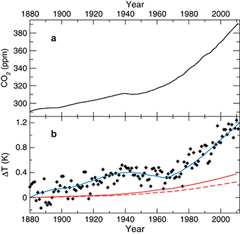
Fig. 4: (a) Reported concentration x(t) of CO2 [34]. (b) Reported increase of the surface temperature by 1.2 K (black diamonds) from 1880 to 2010 [31], fitted curve as a guide for the eye (blue line). Estimated surface temperature change calculated from the spectroscopic properties of CO2 using a 5-layer model for the greenhouse effect (dashed red curve); including the feedback effect of atmospheric water: solid red line.
Download figure:
Standard imageA rough estimate of the global warming by CO2 can be derived from the spectral forcing  that results from the concentration rise via the increase of the spectral efficiency. In the well-known 2-layer model a value of
  is estimated (the more detailed 4-layer model predicts
  ). Treating the surface as a black radiator the thermal re-emission amounts to
  [29]. By differentiation we readily see that the temperature rise
  required to maintain thermal equilibrium is given by
  for
for  .
.
We have computed different global models for the greenhouse effect where radiative equilibrium is considered between the solar input, and the thermal emissions of the surface and the various layers of the atmosphere. Transport phenomena between the layers are included by additional parameters. Our 5-layer model (surface plus 4 atmospheric layers developed in analogy with the scheme shown in fig. 3) predicts reasonable temperatures of approximately 286, 277, 263 and 232 K for the atmospheric parts. The surface temperature of  for
for  is calculated for a proper choice of the solar warming of the atmosphere by
  , while the direct solar input of the surface is taken to be
  (total input
  , global albedo of 0.300). The minor influence of the CO2 increase on the solar input by absorption in the near infrared and leading to the opposite effect of surface cooling is omitted.
Some results for the 5-layer model are presented in fig. 4(b) by the red curves. A direct effect of  is shown for the period 1880–2010 (dashed red line). The simultaneous global warming of the atmosphere, e.g. by 0.15 K for the lowest layer, leads to a growing water content of the atmosphere. The latter effect is omitted in our model computations. As reported by Wang et al. [30] the rising H2O concentration enhances the greenhouse effect by a factor of approximately 1.5. Including this feedback factor leads to the solid red line in the fig. 4(b). Comparing our estimated results with the measured rise of the surface temperature (black data points, fitted blue line) only a modest contribution to the terrestrial warming of less than 33% is derived from the FIR properties of CO2.
The question remains what other factor(s) may be more important for the global temperature increase. A possible source could be the albedo factor (taken to be 0.30 in our calculations). It is obvious that the surface temperature depends on the net solar input reduced by backscattering and reflexion of solar radiation as described by the albedo factor. A decrease by a few percent would be required for a surface warming of 1 K. Changes of the factor of opposite sign  were reported in the years 1985–1997 and 1997–2004 [35,36], without a noticeable effect on the temperature data in fig. 4(b). Other authors provided evidence that the global albedo value remained fairly constant during the past decades [37]. It has been recognized recently that black carbon (BC) in the atmosphere is highly relevant, much more important than the concentration changes of ozone, methane and nitrous oxide [20,38]. As best estimate of industrial-era climate forcing of black carbon a value of
  was obtained and considered to be the second most important human emission after carbon dioxide [39]. The present authors feel that the absorption of environmental pollution in the far infrared should be given more attention. BC absorbs in this spectral region [40,41] and is thus likely to modify the greenhouse effect. Our model calculations suggest that a transmission decrease of 2.3% of the atmosphere in its spectral windows would be sufficient to raise the surface temperature by 1.0 K.
Conclusions
In conclusion we wish to say that we have performed a detailed study of the infrared properties of carbon dioxide to estimate its contribution to the global warming. Our results suggest that CO2 is not predominant for the terrestrial temperature increase. Only a moderate effect of less than 33% is found. Scenarios aiming to reduce further warming should take into account that carbon dioxide is not the dominant cause.