
Abstract
Redox flow batteries (RFBs) are considered an outstanding candidate for the integration of renewable energy sources into the existing power grids. A key property of RFBs is the open circuit voltage (OCV) corresponding to the currentless equilibrium state. In the literature, the Nernst equation describing this property is often simplified by neglecting the activity coefficients. In this work, using a thermodynamically rigorous approach, we show that activity coefficients have a significant influence on the OCV of the Iron-Cadmium and All-Vanadium RFBs. Moreover, this influence varies with the state of charge. Therefore, activity coefficients should not be neglected in the Nernst equation. We show that when doing so, the resulting offset in OCV is actually comparable to typical voltage losses occurring during operation. Hence, fitting kinetic parameters to measurement data of voltage losses can lead to ambiguous results if only the idealized OCV, obtained by neglecting the activity coefficients, is used in that evaluation. Therefore, the implementation of a thermodynamically rigorous model has the potential to significantly improve state-of-the-art models for RFBs.
Export citation and abstract BibTeX RIS
List of symbols
| ai | activity of species i, - |
| b0 | unit molality, 1 mol kg−1 |
| bi | molality of species i, mol kg−1 |
| Ecell | cell voltage, V |

|
standard electrode potential, V |

|
open circuit voltage, V |
| Elosses | voltage losses, V |
| Eex | excess open circuit voltage, V |
| F | Faraday's constant, 96 487 A s mol−1 |
| Ka | dissociation constant, - |
| mi | mass of species i, kg |
| Mi | molar mass of species i, kg mol−1 |
| ni | number of moles of species i, mol |
| N | number of components, - |
| p | pressure, Pa |
| R | universal gas constant, 8.314 J mol−1 K−1 |
| R2 | coefficient of determination, - |
| T | temperature, K |
| zi | charge number of species i, - |

|
molality-based activity coefficient of species i, - |
| η | overpotential, V |
| μi | chemical potential of species i, J mol−1 |

|
molality-based standard chemical potential of species i, J mol−1 |

|
electrochemical potential of species i, J mol−1 |
| νi | stoichiometric coefficient of species i, - |
| Φ | electrostatic potential, V |
| act | activation |
| add | additional |
| i | species i |
| k | functional layer k |
| m, m' | metal phase |
| Me | metal |
| neg | negative electrode |
| ohm | ohmic loss |
| ox | oxidized |
| pos | positive electrode |
| red | reduced |
| rev | reversible |
| tot | total |
| W | water |
Renewable energy sources are currently the fastest growing sources of electricity generation in the world. It is predicted that by 2040 their share will be equivalent to that of coal.1 In contrast to conventional power plants, renewable energy sources such as solar and wind power are intermittent, as the resources are not continuously available for conversion into electricity due to temporal and climatic conditions. Therefore, a stable implementation into the existing power grids is difficult and requires the use of electrical energy storage (EES) systems.2 Redox flow batteries (RFBs) are considered an outstanding candidate among the existing EES systems for stationary energy storage in the grid area, as they offer significant advantages over competing systems (e.g. batteries and supercapacitors), such as independent scaling of power and capacity.2,3
In the 1970s, the Iron-Chromium RFB (Fe/Cr RFB), which is considered the first redox flow battery, was invented and primarily developed by NASA.4 In 1985 the investigations of Sum et al. on the application of the V(II)/V(III) redox pair in the negative half-cell and the V(IV)/V(V) redox pair in the positive half-cell of an RFB were published.5,6 As a consequence, first patents were filed for the All-Vanadium RFB (AVRFB) a few years later. These expired in 2006, which has resulted in renewed interest in commercializing the technology. At present, the AVRFB is the most widely used RFB for large-scale energy storage.7 Several applications already exist, with power outputs ranging from 2 kW to 50 MW and energy capacities from 30 kWh to 250 MWh.8 In recent years, different surface treatments and catalysts were applied to the AVRFB electrodes to increase their reactivity toward redox reactions.9 The main reason for the popularity of the AVRFB is its unique characteristic that all species involved in the redox reactions of both half-cells are vanadium ions. Thus, in contrast to most other RFBs, cross contamination is effectively eliminated.10 In the case of other RFBs, such as the Fe/Cr RFB, dedicated attempts are made to minimize cross contamination by using mixed electrolyte solutions in both half-cells.11 The main disadvantage of the AVRFB is the high cost of vanadium salts. The vanadium in the electrolyte solution accounts for 30%–60% of total system costs.8
Current research on RFBs focuses on increasing energy efficiency and long-term stability, while reducing material and operating costs. There are many design parameters, including e.g. the choice and composition of the electrolyte solution, the electrode and membrane materials, the cell geometry, and flow conditions,4,12–15 so that an accurate mathematical modeling plays a key role in understanding and optimizing RFBs. The employed models differ in their complexity and therefore the computational cost, ranging from simple zero-dimensional16–18 to one-19,20 and two-dimensional21–23 to elaborate and numerically intensive three-dimensional models.24,25 However, in most studies only the AVRFB is considered, since its development is most advanced compared to other RFB types.
A key objective in modeling RFBs is the cell voltage. It can be calculated from the Nernst equation describing the open circuit voltage (OCV) at electrochemical equilibrium and adding terms for voltage losses. These losses consist of ohmic losses and overpotentials (e.g. activation overpotential, reaction overpotential or concentration overpotential).26 Recent models of RFBs differ in their treatment of the overpotentials.16–18 For example, the equation for the calculation of the cell voltage Ecell used in the zero-dimensional model according to Sharma et al.17 is
Here,  is the OCV calculated from the Nernst equation (see below),
  are ohmic losses in different parts k of the RFB (e.g. membrane, electrolyte, current collectors), and
  and
and  are activation overpotentials in the positive and negative electrodes, respectively. It is obvious that when adjusting model parameters for the loss terms in Eq. 1 to measurement data for Ecell, the outcome depends on how the OCV is calculated. In general, the OCV depends only on the reacting redox pair, the overall composition of the electrolyte solution, and the temperature.27 In contrast, the voltage losses Elosses are also influenced by the design of the RFB (cell geometry, flow conditions, electrode and membrane materials).
The OCV of a RFB can be calculated using the Nernst equation, which is given by
where  is the standard cell potential, R is the universal gas constant, T is the temperature, z is the number of electrons transferred in the cell reaction, N is the number of components of the cell reaction, and b0 = 1 mol kg−1 is the unit molality. Furthermore, ai, bi,
  , and νi are the activity, molality, activity coefficient on the molality scale, and stoichiometric coefficient of component i (νi > 0 for products and νi < 0 for reactants), respectively.
The correct application of the Nernst equation to RFBs has been the subject of substantial debate in the literature. There were even discussions which species should be considered in Eq. 2. As an example, when modeling AVRFBs it was common to neglect the proton molalities,21,28,29 until Knehr and Kumbur30 and Gandomi et al.31 stressed that this approach is invalid. From a thermodynamic standpoint, however, it is clear that all species taking part in the half-cell reactions must appear in the Nernst equation.
Moreover, it is common practice in the literature to neglect the activity coefficients  of the species that appear in the Nernst equation, i.e. setting
  for all i, although highly concentrated, multicomponent aqueous electrolyte solutions are usually employed in RFBs. Lenihan et al.10 estimate the water activity of electrolyte solutions employed in AVRFBs to be in the range 0.6–0.8, which corresponds to a highly non-ideal solution. To the best of our knowledge, only Muñoz et al.32 emphasize the importance of activity coefficients for a more accurate prediction of the OCV. They introduce a "global activity coefficient" as a correction to the neglect of the activity coefficients of the individual species, which, however, can only be determined by fitting to measurement data. In several studies, the collective effect of the activity coefficients is combined into a so-called "formal potential term", commonly measured at state of charge (SOC) of 50%.33–35 However, activity coefficients in electrolyte solutions are very sensitive to the concentration. This has two consequences: First, the "formal potential term" must be measured whenever the initial composition of the electrolyte solution is changed. This is important e.g. when studying different concentrations of the vanadium species or testing a different supporting electrolyte. Second, and more importantly, the results of the present work show that the "formal potential term" actually changes with the SOC. Therefore, it cannot be simply added to the standard cell potential as a constant offset.
Hence, the central aspect of the present work will be the last term in Eq. 2. Since it considers the influence of activity coefficients on the OCV and thus stems from the excess chemical potential, that term will be called "excess OCV" from here on and designated with the symbol Eex. It is defined as
Denoting the two remaining terms in Eq. 2 by  yields
In this work, a model for the exact prediction of the OCV for different RFB types is developed, focusing mainly on the Iron-Cadmium RFB (Fe/Cd RFB). The reason for this choice is that a reliable thermodynamic model for this electrolyte system is available in the literature, namely the Pitzer model. Unfortunately, a thermodynamically rigorous model cannot be built in the same way for the AVRFB due to a lack of necessary model parameters or data from which these parameters could be obtained. Nevertheless, based on experimental data of the OCV of an AVRFB from the literature, the influence of the activity coefficients on the OCV over the SOC can be determined. Additionally, the developed model is used to investigate the sensitivity of the OCV on the composition of the electrolyte solution of the Fe/Cd RFB, again comparing the "ideal" (all  ) to the "real" (
 from a thermodynamic model) treatment. Furthermore, voltage losses during operation of the RFB are investigated using measurement data and existing models from the literature.
This work is organized as follows: The considered RFB types and the proposed model for the OCV calculation is explained in the Model development section. Following this, an overview of the scenarios studied in the present work is given in the Simulation section. The findings obtained from these scenarios are then discussed in the Results and Discussion section, before conclusions are drawn. The supplementary material (available online at stacks.iop.org/JES/167/110516/mmedia) contains some technical details of the calculations and an overview of electrochemical thermodynamics for the reader's reference. A more detailed review of the latter was recently given in Ref. 36.
Model Development
Considered RFB types
Overview
As there are many articles in which the functionality of RFBs is described excellently, e.g. Ref. 34, we refrain from including such a description here. In this work, two types of RFBs were investigated, namely the AVRFB and the Fe/Cd RFB. In addition, two different compositions of the electrolyte solutions were considered for the Fe/Cd RFB. The main purpose of the developed mathematical model is the accurate calculation of the OCV of these RFBs. However, the methodology can be easily applied to other RFB types, given that all necessary parameters are available. We note here that only those reactions which are explicitly given in the text are included in the model. Side reactions are neglected and would otherwise have to be implemented in the model in the same way as the considered ones. Furthermore, we assume that all electrolyte solutions are well mixed to attain the state of equilibrium.
AVRFB
In the case of the AVRFB, the positive electrolyte solution tank contains  and VO2+ ions and the negative electrolyte solution tank contains V3+ and V2+ ions, which corresponds to vanadium in the oxidation states V, IV, III, and II. In addition, a supporting acid, which is typically sulfuric acid for the AVRFB, is added to increase the solubility of the salts and the conductivity of the electrolyte solution. The chemical reactions on the electrodes of the two half-cells and their potential vs the standard hydrogen electrode (SHE) can be expressed as Ref. 37
Combining the reactions (I) and (II) leads to the total cell reaction of the AVRFB:
Fe/Cd RFB
In addition to the established RFBs, the combination of different half-cell reactions and variations in the composition of the electrolyte solutions result in a very large number of other possible RFB designs. A new promising candidate is the Fe/Cd RFB developed by Zeng et al.,38 which showed a small capacity reduction during the cycle test and low predicted costs for energy storage. In contrast to the AVRFB, the same initial electrolyte solution, which is an aqueous solution of FeCl2 and CdCl2 with HCl as the supporting acid, is typically used in both half-cells. The cell is equipped with a cation exchange membrane through which only H+ can diffuse. The Fe/Cd RFB is a hybrid RFB, i.e. a solid is formed during charging: at the negative electrode, cadmium metal is dissolved and redeposited. The chemical reactions occurring in the half-cells of the Fe/Cd RFB can be expressed as Ref. 38
Combining the reactions (IV) and (V) leads to the total cell reaction of the Fe/Cd RFB:
Mass balance
Overview
The properties of RFBs are usually described as a function of the SOC. Throughout the present work, the SOC is defined as
where  represents the molality of the active metal species (Me) in the positive half-cell (pos) in oxidized form and
  in reduced form. Hence, an SOC of 1 corresponds to a fully charged RFB, and an SOC of 0 corresponds to a fully discharged RFB. It is also possible to define the SOC with respect to the molalities in the negative half-cell, which leads to an expression equivalent to Eq. 5. In the literature, sometimes molarities are used to define the SOC instead of molalities.18,20
Furthermore, for both RFBs considered in this work, the following mass balances, which can be derived from Eq. 5, are applicable:


An additional necessary assumption for the derivation of Eqs. 8 and 9 is

where  and
and  are the total number of moles of the active metal species in the positive and negative half-cells. Furthermore,
  and
and  are the numbers of electrons transferred per mole of metal species in the positive and negative half-reaction, respectively. Equation 10 is valid for all the compositions of the electrolyte solutions described in this work (see Table I) and ensures that the capacity of both half-cells is the same. Therefore, at an SOC of 0 and 1, only one species of the corresponding redox couple is present in both the positive and negative half-cells. In the case of the two RFBs considered in this work, Eq. 10 leads to

for the AVRFB and

for the Fe/Cd RFB.
Table I. Overview of scenarios studied in the present work.
| # | RFB type | Overall composition | Membrane | Pitzer parameters | Objective |
|---|---|---|---|---|---|
| 1 | Fe/Cd RFB |
 = 1.0 mol l−1 = 1.0 mol l−1 |
catex | complete | Simulation of  and and 
|
 = 0.5 mol l−1 = 0.5 mol l−1 |
with the developed model | ||||
 = 3.0 mol l−1 = 3.0 mol l−1 |
|||||
| 2a | AVRFB |
 = 2.0 mol l−1 = 2.0 mol l−1 |
catex | unavailable; | Simulation of  and and |
 = 3.0 mol l−1 = 3.0 mol l−1 |
no activity based | comparison with measured  data37 data37 |
|||
 = 1.0 mol l−1 = 1.0 mol l−1 |
model used | ||||
 = 2.0 mol l−1 = 2.0 mol l−1 |
|||||
| 2b | AVRFB |
 = 1.6 mol l−1 = 1.6 mol l−1 |
anex | unavailable; | Simulation of  and and |
 = 3.2 mol l−1 = 3.2 mol l−1 |
no activity based | comparison with measured  data37 data37 |
|||
 = 0.8 mol l−1 = 0.8 mol l−1 |
model used | ||||
 = 0.8 mol l−1 = 0.8 mol l−1 |
|||||
| 3 | Fe/Cd RFB | varied | catex | complete | Sensitivity analysis |
| 4 | Fe/Cd RFB |
 = 1.0 mol l−1 = 1.0 mol l−1 |
catex | complete | Calculation of voltage losses using |
 = 0.5 mol l−1 = 0.5 mol l−1 |
(except  ) ) |
measured Ecell data38 | |||
 = 3.0 mol l−1 = 3.0 mol l−1 |
|||||
All salts are assumed to dissociate completely. Furthermore, it is assumed that hydrochloric acid dissociates completely according to

In the case of sulfuric acid, only the first dissociation step is considered to be complete, while the incomplete dissociation of bisulfate is captured via its dissociation equilibrium constant:
The thermodynamic equilibrium constant of reaction (IX) (Ka = 1. 05 · 10−2 at 298.15 K and 1 bar) is taken from the literature.39 More details on the calculation of this dissociation equilibrium are provided in the supplementary material.
AVRFB
In case of the AVRFB, the SOC (see Eq. 5) is defined as
By applying Eqs. 6–9 to an AVRFB with cation exchange membrane, in which protons diffuse freely between the two half-cells, Eqs. 14–17 are obtained.


In addition to the metal ions, the molality of the protons in the two half-cells is crucial for the calculations. During operation of the RFB, this molality varies and is influenced by  , which represents the amount of additional protons due to redox reactions and diffusion through the membrane. In the positive half-cell, two moles of protons are formed per mole of
  during charging (see reaction (I)). At the same time, one mole of protons diffuses through the cation exchange membrane into the negative half-cell. Here,
  is defined relative to a fully discharged RFB (SOC = 0). Of course, the actual proton concentration also depends on the overall acid concentration and the dissociation equilibrium of the corresponding acid (see reactions (VII)–(IX)).
Water is formed in the positive half-cell of the AVRFB during discharge. The mass balance of water in this case can be expressed as
where  is the mass of water in the positive half-cell at an SOC of 0 and MW is the molar mass of water. Inserting Eq. 14 into Eq. 20 and rearranging yields
In the case of an AVRFB setup with an anion exchange membrane,  ions instead of protons can diffuse freely between the two half-cells. Therefore, in this case, Eqs. 18 and 19 have to be replaced by the following relationships:


Fe/Cd RFB
In case of the Fe/Cd RFB, the SOC is defined as
By applying Eqs. 6–9 to an Fe/Cd RFB with cation exchange membrane, the following mass balances are obtained:


Since diffusion of water across the membrane is neglected, a constant amount of solvent can be assumed for the Fe/Cd RFB with the result that  and
and  always equal their initial values. This assumption is not valid for the AVRFB due to the formation of water at the positive half-cell during discharge.
Nernst equation
For the Fe/Cd RFB, the Nernst equation was derived in the present work (see Appendix) and is given by
For the AVRFB, the Nernst equation was derived by Pavelka et al.37 In case of a cation exchange membrane, it is given by
If an anion exchange membrane is used in an AVRFB instead of the cation exchange membrane, Eq. 33 is replaced by
Activity coefficient model
The investigated RFBs employ electrolyte solutions with high concentrations of salts and acids. A suitable thermodynamic model must be chosen for describing these solutions appropriately. In the present work, the Pitzer model is applied, which was implemented as suggested by Bea et al.40 In the literature, there is a plethora of models for activity coefficients in electrolyte solutions, which differ in their complexity and the number of adjustable parameters. In this work, the Pitzer model41–45 is used to describe the activity coefficients, as it was developed especially for aqueous multicomponent solutions and has proven to yield reliable predictions at high ionic strengths.46 All necessary model parameters for the simulations conducted in this work are taken from the literature and listed in the supplementary material. When selecting the parameters, care was taken to ensure that the concentrations used in the RFBs do not exceed the maximum molality of the parameterization data. Typically, Pitzer parameters are only available for room temperature (25 °C), which must be taken into account.
The composition of the electrolyte solution is frequently reported in molarities. However, since the Pitzer model is formulated in molalities, a conversion of the concentrations is necessary. For this purpose, overall molarities were converted into molalities using the formulae and tabulated data given in the supplementary material.
Simulation
The model described in the previous section was implemented in MATLAB® R2018a.47 Using the mass balances, dissociation equilibria, the Pitzer model, and the Nernst equation described therein, the OCV was calculated. The temperature and the overall composition of the electrolyte solution are necessary as input variables. Many of the input parameters of the model depend on temperature, e.g. the standard electrode potentials  , the dissociation constants Ka, and the Pitzer parameters (see supplementary material). All calculations in the present work are carried out for 298.15 K. By selecting suitable input data, the developed model can be used to investigate many further RFB types and state conditions.
An overview of the simulations carried out in the present work is presented in Table I, together with an overview of the RFB setups and Pitzer parameter sets. The electrolyte compositions were chosen according to experimental studies available in the literature.37,38 In addition, the sensitivity of the OCV of the Fe/Cd RFB with respect to the overall composition of the electrolyte solution was investigated.
To provide an insight into the reasoning behind the choice of studied scenarios, these scenarios are discussed in the following with respect to their objectives. The currentless state of equilibrium, i.e. the modeling of the OCV, is considered in scenarios #1, #2, and #3. In these scenarios, both the ideal ( ) and the real case (
 from a thermodynamic model) were studied and compared. The compositions of the electrolyte solutions are taken from experimental investigations of the different RFBs from the literature (Zeng et al.38 for the Fe/Cd RFB and Pavelka et al.37 for the AVRFB). For the Fe/Cd RFBs, the overall compositions of the electrolyte solutions are usually the same in both half-cells to minimize the risk of cross contamination.
After the evaluation of the results with the typical overall molarities for the Fe/Cd RFB discussed in scenario #1, the sensitivity of the OCV to variations in the composition of the electrolyte solution was investigated in scenario #3. Again, the ideal and real cases were studied and compared. In scenario #3, the overall molarity of hydrochloric acid was varied between 1.0 and 5.0 mol l−1 (typical value: 3.0 mol l−138) and that of iron chloride was varied between 0.1 and 3.0 mol l−1 (typical value: 1.0 mol l−138). The overall CdCl2 molarity was always half that of FeCl2. In experiments on stability of electrolyte solutions, Zeng et al.38 showed that a composition with chloride salts only is less stable than a composition with sulfate salts and tends to form solid precipitates at higher overall metal concentrations (twice as high as in scenario #1 in Table I). At the higher electrolyte concentrations considered in the sensitivity analysis, precipitation might occur. However, this was not further investigated in the present work. All electrolyte solutions were assumed to be stable. Scenario #4 is used to evaluate typical voltage losses that occur during operation of the RFB. Measurement data of the cell voltage of a Fe/Cd RFB were examined and compared with the simulation results of the OCV.
In the following, the studied scenarios are briefly discussed with respect to the availability of Pitzer parameters. The electrolyte solution for the Fe/Cd RFB with chloride salts only studied in scenario #1 was chosen because all Pitzer parameters needed for the calculations are available. Pitzer parameters are not available for the vanadium salts used in AVRFBs, therefore the real OCVs in scenario #2 were estimated using measurement data for setups with a cation exchange (catex) and an anion exchange (anex) membrane. We note briefly here that a model for volumetric properties of solutions used in AVRFBs based on variants of the Pitzer equations is available in the literature,48 but this model can of course not be used for the calculation of activity coefficients.
Results and Discussion
OCV of the Fe/Cd RFB
In scenario #1, a Fe/Cd RFB with chloride salts only was studied, see Table I. Figure 1a shows the OCV curves for the ideal ( ) and real case (
 calculated with the Pitzer model) as functions of the SOC.
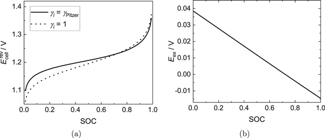
Figure 1. (a) OCV of the Fe/Cd RFB with chloride salts only as a function of the SOC calculated with the present model. Dotted line: ideal case (neglect of activity coefficients), solid line: real case (activity coefficients from Pitzer model). (b) Excess OCV (Eex) of the Fe/Cd RFB with chloride salts only according to Eq. 3 as a function of the SOC.
Download figure:
Standard image High-resolution imageAs could be expected from the high concentrations of ionic species, a significant difference between the two curves corresponding to the ideal and the real case is found. The observed difference in the OCVs is solely caused by the influence of the activity coefficients, i.e. by the excess OCV Eex, which can be calculated using Eq. 3 and which is plotted in Fig. 1b. Therefore, activity coefficients should not be neglected in the Nernst equation.
When modeling the OCV of RFBs, it is often assumed that the ratio of activity coefficients and thus also Eex remains constant over the SOC, so that this contribution may simply be viewed as an additional additive contribution to the OCV, the so-called "formal potential term".33–35 The present results show that this is not the case. By contrast, the excess OCV depends linearly on the SOC, with a coefficient of determination of about R2 = 0.99998. In the supplementary material, a possible reason for the linear trend of the excess OCV vs the SOC in the case of the Fe/Cd RFB is presented. There, the natural logarithm of all species' activity coefficients is shown as a function of the SOC. For most species, that property depends approximately linearly on the SOC. Consequently, when summing up these terms in the Nernst equation that linearity is preserved. However, we can only investigate this thoroughly for the Fe/Cd RFB, so that we cannot make any predictions whether this is only a peculiarity of the Fe/Cd RFB or a generic feature of RFBs.
Moreover, Eex varies between 0.038 V (SOC  0) and −0.014 V (SOC
  1). Thus, it is in the same order of magnitude as the voltage losses during operation, which are discussed in more detail below.
OCV of the AVRFB
For the AVRFB, no Pitzer parameters are available. Thus, the calculation presented in the previous subsection cannot be simply repeated for the AVRFB. However, measurement data of the OCV are available,37 which can be used to estimate the excess OCV.
In the experiments conducted by Pavelka et al.,37 two AVRFB setups were investigated: one with a catex and one with an anex membrane. Both setups are considered here, see scenarios #2a and #2b in Table I, using the reported overall compositions by Pavelka et al.37
Figures 2a and 3a show the measured OCV data by Pavelka et al.37 in comparison to the ideal OCV calculated with the present model. Additionally, the simulation results of the ideal OCV of Pavelka et al. are shown. Their calculations differ from the ones presented here in terms of the mass balances and the dissociation equilibrium of sulfuric acid, for which Pavelka et al. made additional assumptions. In the present work, the dissociation equilibrium is treated in a thermodynamically rigorous way. Furthermore, Figs. 2b and 3b show the calculated excess OCV (see Eq. 3), which is the difference between the measured (real) OCV and the simulated (ideal) OCV illustrated in Figs. 2a and 3a.
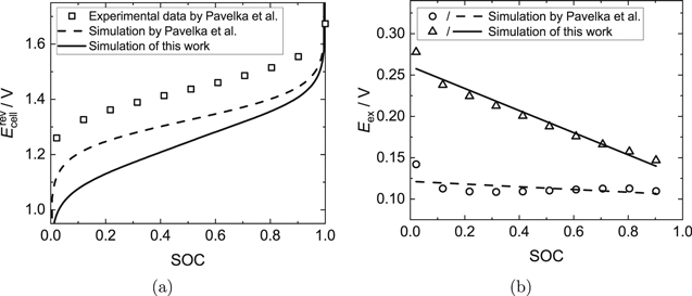
Figure 2. AVRFB with a catex membrane. (a) Comparison of the simulated ideal OCV according to Pavelka et al.37 (dashed line), the simulated ideal OCV from this work with explicit treatment of the dissociation of sulfuric acid (solid line) and the experimental real OCV data from Pavelka et al. (open symbols). The activity coefficients were neglected in the simulations. (b) Difference between the experimental data from Pavelka et al.37 and the simulated OCV according to Pavelka et al. (circles) or the simulated OCV with explicit treatment of the dissociation of sulfuric acid (triangles), as presented in (a). In addition, linear fits of the data are shown (dashed line: R2 = 0.23217; solid line: R2 = 0.95588).
Download figure:
Standard image High-resolution image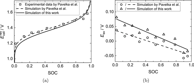
Figure 3. AVRFB with an anex membrane. (a) Comparison of the simulated ideal OCV according to Pavelka et al.37 (dashed line), the simulated ideal OCV from this work with explicit treatment of the dissociation of sulfuric acid (solid line) and the experimental real OCV data from Pavelka et al. (open symbols). The activity coefficients were neglected in the simulations. (b) Difference between the experimental data from Pavelka et al.37 and the simulated OCV according to Pavelka et al. (circles) or the simulated OCV with explicit treatment of the dissociation of sulfuric acid (triangles), as presented in (a). In addition, linear fits of the data are shown (dashed line: R2 = 0.83265; solid line: R2 = 0.89589).
Download figure:
Standard image High-resolution imageAs illustrated in Figs. 2 and 3, the simulated ideal OCVs for the setup with a catex membrane deviate significantly from the measured data, while in the case of the setup with an anex membrane, the differences are moderate, but still important. The maximum excess OCV is 0.28 V (SOC  0) for the setup with the catex membrane and 0.08 V (SOC
  0) for the setup with the anex membrane, which is significantly higher than for the Fe/Cd RFB discussed in the previous subsection. Furthermore, the changes of the excess OCV over the SOC shown in Figs. 2b and 3b are larger than in the simulation results of the Fe/Cd RFB.
In this work, the dissociation equilibrium is treated in a thermodynamically rigorous way, but since the activity coefficients cannot be calculated due to a lack of Pitzer parameters, some uncertainties as to the reliability of the calculations remain and it is not possible to estimate the accuracy of the simulation results. It can only be noted that the developed model yields lower ideal OCVs for both simulated setups and thus larger excess OCVs than the model of Pavelka et al.37 Thus, the treatment of the dissociation equilibrium of sulfuric acid has a crucial influence on the OCV. Nevertheless, both sets of calculations, i.e. those of Pavelka et al. and those of the present work, indicate that the assumption of a constant excess OCV Eex32,34 is not valid.
Evaluation of the regression lines obtained with the present model support the assumption that the dependence of Eex on the OCV could be described more accurately by a straight line, which validates the findings for the Fe/Cd RFB in the previous subsection.
Sensitivity of the OCV on the composition of the electrolyte solution of the Fe/Cd RFB
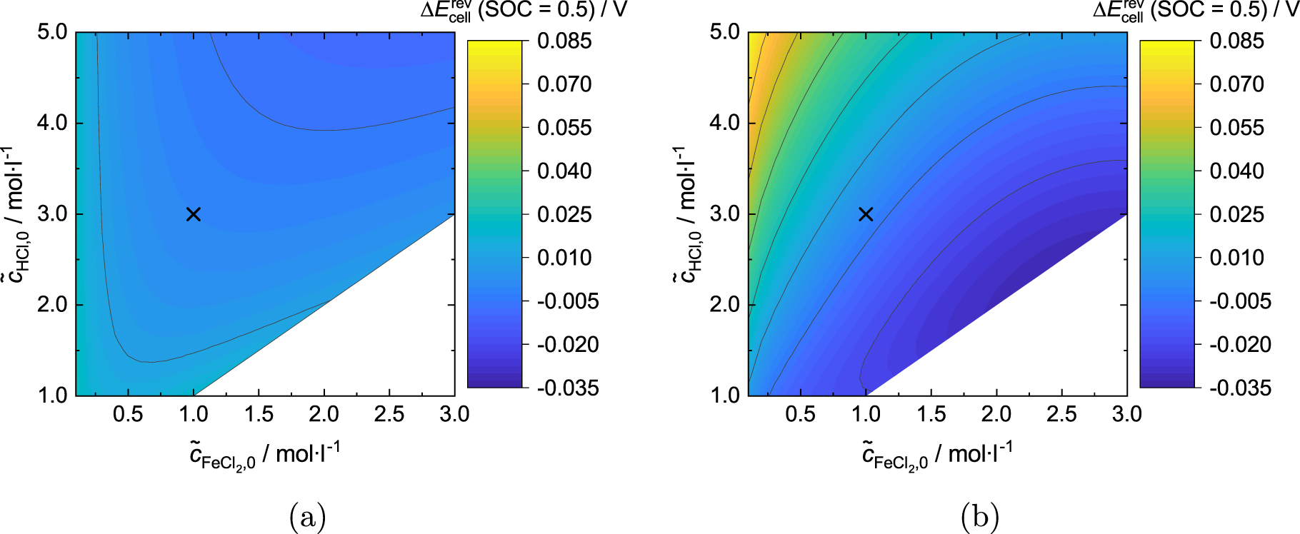
In this subsection, an optimization of the composition of the electrolyte solution toward high OCVs as described in scenario #3 in Table I is discussed. In order to investigate the influence of activity coefficients on the results, the ideal and real OCV plots are compared. The contour plots shown in Fig. 4 summarize the results of the variation of the overall salt molarities and the variation of the overall HCl molarity. There, the OCV at an SOC of 0.5 is shown as an example, which is, however, representative for most of the entire SOC range (except for very high SOC).

Figure 4. Simulated OCV at an SOC of 0.5 with variation of the overall molarities of FeCl2 between 0.1 and 3.0 mol l−1 and of HCl between 1.0 and 5.0 mol l−1. The overall CdCl2 molarity is always half that of FeCl2. The cross indicates the typical overall composition of the electrolyte solution of the Fe/Cd RFB with chloride salts only (see scenario #1 in Table I 38). No simulation data can be generated for the white area, since the quantity of protons is not sufficient for charge equalization over the entire SOC. (a) Ideal case (neglect of activity coefficients). (b) Real case (activity coefficients from Pitzer model).
Download figure:
Standard image High-resolution imageFor both the ideal and the real case, the model predicts that lower overall salt molarities lead to a higher OCV. In contrast, the variation of the HCl molarity shows different trends for the ideal and real cases: while the OCV rises with increasing HCl molarity in the ideal case, the real case predicts the opposite (except for very low acid molarities at high SOC). Hence, neglecting the activity coefficients is misleading when optimizing the OCV by varying the electrolyte composition: looking at the ideal case suggests lowering the acid concentration is beneficial, while in reality, the opposite is true.
In Fig. 5, the results already shown in Fig. 4 are depicted in a different way to show the difference of the OCV between the typical operating point (cross) and other operating conditions: there, the same color scale is used for both the ideal and real cases. That color scale is set to zero for the typical operating point of the Fe/Cd RFB, see scenario #1 in Table I. Figure 5 illustrates which overall compositions of the electrolyte solutions could enhance the OCV and shows the absolute difference to typical concentrations used in Fe/Cd RFBs.38 The influence of the variation is assumed to be much smaller in the ideal case than it is in the real case. Hence, the full optimization potential of the RFB is underestimated if only the ideal part of the Nernst equation is taken into account.

Figure 5. Deviations of the OCV at an SOC of 0.5 from the typical operating point (cross; see scenario #1 in Table I 38) of the Fe/Cd RFB with chloride salts only. Variation of the overall molarities of FeCl2 between 0.1 and 3.0 mol l−1 and of HCl between 1.0 and 5.0 mol l−1. The overall CdCl2 molarity is always half that of FeCl2. No simulation data can be generated for the white area, since the quantity of protons is not sufficient for charge equalization over the entire SOC. (a) Ideal case (neglect of activity coefficients). (b) Real case (activity coefficients from Pitzer model).
Download figure:
Standard image High-resolution imageInfluence of the excess OCV on voltage losses in the Fe/Cd RFB
RFBs during operation are considered in the following as described in scenario #4 in Table I, in contrast to the currentless state of equilibrium discussed above. Measurement data provided by Zeng et al.38 are compared with calculated OCVs to estimate the occurring voltage losses. The measurement data of Zeng et al.38 were carried out with a Fe/Cd RFB with chloride and sulfate salts. For this system, one set of Pitzer parameters, namely those of the Cd2+- interaction, are not available. In principle, this can lead to inaccuracies in modeling the activity coefficients. However, as the concentration of Cl− ions in the investigated RFB is typically 10 times larger than that of the
  and
and  ions, the impact of the missing parameters is presumably rather small. Furthermore, the binary parameters of all other combinations of anions and cations of the described electrolyte solution are available.
Zeng et al.38 reported measured cell voltage data during charging of a Fe/Cd RFB as a function of time for four different current densities. Furthermore, the electrolyte utilization at the cutoff voltage (1.35 V) is given for each case. Explanations for the relatively low electrolyte utilization are already provided by Zeng et al.38 and are not discussed here. Based on the reported data, the cell voltage curves as a function of the SOC (see Eq. 25) were derived. In terms of the SOC definition used in the present work, the charging experiments by Zeng et al. start at SOC = 0. The SOC at the end of the experiment can be determined from the electrolyte utilization provided by Zeng et al.,38 in the following we discuss only the current densities 40 mA cm−2 and 160 mA cm−2.
The data of the charge process provided by Zeng et al.38 show that the measured cell voltage rises with increasing current density, which is due to current-dependent voltage losses during charging of the RFB. As outlined in the introduction, the voltage losses are calculated as

where Elosses,real is the true sum of all voltage losses, i.e. considering the activity coefficients when calculating the OCV. Hence, inaccuracies in the calculation of the OCV, such as the neglect of activity coefficients, lead to errors in the calculation of voltage losses. To distinguish the two approaches, the term Elosses,ideal is introduced in the following as

to indicate the losses that one would expect when calculating the OCV without activity coefficients. Combining Eqs. 4, 35 and 36 yields
Equation 37 clearly shows that the neglect of the excess OCV leads to erroneous estimations of the voltage losses.
Figures 6a and 7a illustrate the comparison of the simulated ideal and real OCV with the measurement data of Zeng et al.38 for the two applied current densities. Furthermore, Figs. 6b and 7b show the ideal and real voltage losses calculated from the data in Figs. 6a and 7a, as well as the excess OCV.

Figure 6. Applied current density: 40 mA cm−2. (a) Comparison of measurement data of a Fe/Cd RFB by Zeng et al.38 with simulation results using the model developed in the present work for the OCV. Model calculations were performed for the ideal (neglect of activity coefficients) and the real case (activity coefficients from Pitzer model). (b) Estimated ideal and real voltage losses (see Eqs. 35 and 36) of the Fe/Cd RFB investigated by Zeng et al.38 In addition, the excess OCV calculated using Eq. 3 is shown.
Download figure:
Standard image High-resolution image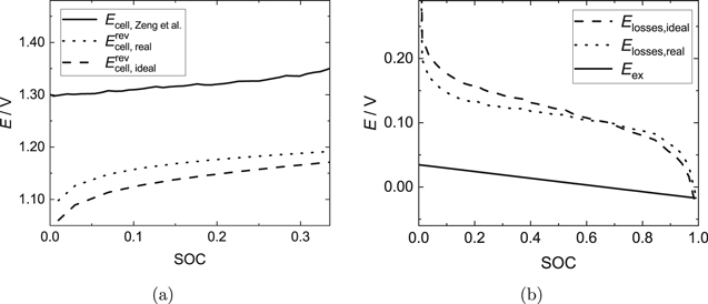
Figure 7. Applied current density: 160 mA cm−2. (a) Comparison of measurement data of a Fe/Cd RFB by Zeng et al.38 with simulation results using the model developed in the present work for the OCV. Model calculations were performed for the ideal (neglect of activity coefficients) and the real case (activity coefficients from Pitzer model). (b) Estimated ideal and real voltage losses (see Eqs. 35 and 36) of the Fe/Cd RFB investigated by Zeng et al.38 In addition, the excess OCV calculated using Eq. 3 is shown.
Download figure:
Standard image High-resolution image
The excess OCV describes the equilibrium state and is therefore only a function of the SOC, but does not depend on the applied current density. At an applied current density of 40 mA cm−2, the calculated voltage losses are small and in the order of magnitude of the excess OCV. Hence, when calculating voltage losses with respect to  , an appreciable error can be made: the voltage losses can be under- or overestimated to a large extent. Higher applied current densities lead to increasing voltage losses caused by overpotentials and ohmic losses, so that the relative difference between ideal and real voltage losses decreases. Therefore, the thermodynamically rigorous calculation of the OCV is especially important when studying voltage losses in RFB setups at low current densities.
In the literature, the experimental data of ideal voltage losses of lab-scale RFB setups are often used to adjust model parameters, e.g. the kinetic parameters in the Butler-Volmer equations for the calculation of activation overpotentials.17,22,23,28,49,50 However, the present results indicate that the ideal voltage losses under- or overestimate the real voltage losses. As a result, the obtained fit parameters have to effectively capture phenomena that should rather be included in the description of the equilibrium state. Both the voltage losses and the excess OCV depend on the SOC, but not necessarily in the same functional form. Even if they did, that functional form would not be known. The excess OCV and the voltage losses (see Eq. 1) should therefore be treated independently. Hence, a precise calculation of the OCV can help to evaluate the required fit parameters more accurately for a wide range of operating regimes in order to improve existing models.
For the AVRFB, the calculations presented in this subsection cannot be simply repeated due to a lack of necessary Pitzer parameters or data from which these parameters could be obtained. Instead, we implemented the zero-dimensional model by Sharma et al.17 to get an estimate of the magnitude of the different types of voltages losses. The predicted types of voltage losses (activation overpotentials and ohmic losses of the current collector, electrolyte, and membrane) are smaller or of the same magnitude as the estimated excess OCV of a typical AVRFB examined above. This supports the hypothesis that activity coefficients are essential for an accurate modeling of RFBs and should not be neglected.
Conclusions
In this work, the hypothesis was investigated that considering activity coefficients in electrolyte solutions is essential for the modeling of RFBs. By simulating a Fe/Cd RFB and using measurement data from an AVRFB, it could be demonstrated that the excess OCV is substantial and should not be neglected. Moreover, in contrast to a common assumption in the literature, the excess OCV is not a constant, but rather varies with the SOC. Our results for both RFBs show a linear relationship between the excess OCV and the SOC, however, this linear dependence is not necessarily a unique feature for all RFBs. Nonetheless, these results show that the introduction of a so-called "formal potential term" is thermodynamically invalid. Furthermore, using measurement data from a Fe/Cd RFB during operation, it was shown that voltage losses are in the same order of magnitude as the excess OCV, so that their estimation depends strongly on the way the OCV is calculated. With this new approach, this work proves that activity coefficients have a significant influence on the modeling of RFBs that should not be neglected.
Additionally, the developed model provides the framework for conducting sensitivity studies. This was demonstrated by investigating the sensitivity of the OCV of a Fe/Cd RFB on the composition of the electrolyte solution. The observed dependencies of the OCV on the overall molarities of the electrolyte solutions would be misinterpreted if activity coefficients were neglected. Potentially, the obtained results can be used to optimize the composition of the electrolyte solution of a Fe/Cd RFB. In the present work, the solubilities of the electrolytes and the stability of the RFB electrolyte solution was not considered. Therefore, in future applications of the model, e.g. for multicriteria optimization of the composition of the electrolyte solution, a calculation of the electrolyte solubilities should be added.
The results of the present work indicate that in future work, activity data of the electrolyte solutions in the AVFRB should be measured, and a thermodynamic model, e.g. the Pitzer model, should be fitted to these data. In literature models, the required parameters for voltage losses are usually obtained by a fit to data of lab-scale RFB setups, a procedure which is prone to errors due to an inaccurate OCV calculation. Therefore, implementing a thermodynamically accurate model to describe the electrolyte solutions used in RFBs has the potential to significantly improve the simulations of the OCV, the cell voltage, and voltage losses, thus improving the understanding of RFBs in general and allowing for a more robust cell design.
: Appendix: Derivation of the OCV of a Fe/Cd RFB
In the following, the Nernst equation for describing the OCV of a Fe/Cd RFB is derived. The approach is similar to that of Pavelka et al.37 and Muñoz et al.32 for the AVRFB. Chemical equilibrium for both half-cell reactions (IV) and (V) (see Model development section) is given by the equality of the electrochemical potentials:
Here, m and m' represent the phase of the wires connecting the voltmeter and the terminals of the battery.32 By inserting the definition of the electrochemical potential (see supplementary material) into A·1 and A·2, the following equations are obtained:

Since a proton-permeable catex membrane is used, the electrochemical potential of protons has to be the same in both half-cells,37 resulting in
Combining Eqs. A·3–A·5 leads to
An appropriate normalization (see supplementary material) of the electrochemical potentials in Eq. A·6 yields
Furthermore, the standard electrode potentials of both half-cells38 can be expressed as
leading to the standard electrode potential of the Fe/Cd RFB
Finally, inserting Eqs. A·8–A·10 into A·7 gives the result
Equation A·11 is the thermodynamically rigorous Nernst equation for the Fe/Cd RFB.