

Abstract
Measuring carbon (C) loss through different pathways is essential for understanding the net ecosystem exchange of carbon dioxide (CO2) in tidal wetlands, especially in a reality where wetland mitigation and protecting coastlines from rapid sea-level rise is a growing priority. Tracking C loss can help reveal where an ecosystem is storing the most C, but it can also help scientists understand near- and long-term impacts of wetland restoration on climate. A recently developed partial pressure of dissolved CO2 platform was tested in a subtropical salt marsh with an apparatus that raised and lowered sensor housing with the tide. Additional low-cost water quality sensors were installed nearby for measuring turbidity and salinity. Here, we evaluated how well this floating sensor platform along with 28 d of biogeochemical data from a tidal salt marsh could detect C import and export from tidal effects. This work provides a pathway to low-cost, routine in-situ C exchange measurements which serve the needs of environmental managers, researchers, and others interested in better estimating wetland C storage and transport.
Export citation and abstract BibTeX RIS

Original content from this work may be used under the terms of the Creative Commons Attribution 4.0 license. Any further distribution of this work must maintain attribution to the author(s) and the title of the work, journal citation and DOI.
Corrections were made to this article on 29 August 2023. An author affiliation was updated.
1. Introduction
Nearly three quarters of all inorganic and organic carbon (C) sequestrated and exported from terrestrial inland waterways and wetlands is evaded to the atmosphere as carbon dioxide (CO2) before the time it reaches the ocean (Ward et al 2017). For much of this C transport, mangroves and tidal marshes represent the last stop on this journey for potential organic C sequestration while also being the first natural defense against sea level rise due to soil accretion, soil expansion, and the presence of coastal vegetation (Mudd et al 2010, Macreadie et al 2019). Tidal wetland C gains are expected in future climate scenarios in the US, Australia, Brazil, and China, while losses are expected in Indonesia and Mexico due to changes in wetland area (Wang et al 2021). Coastal ecosystems play an important role in the C cycle despite their small surface area, transforming and storing significant amounts of C in marine sediment (Kirwan and Megonigal 2013). However, environmental and human-caused stressors are projected to cause disappearance of these ecosystems and jeopardize their role as C sinks in the global C cycle (Lovelock and Reef 2020).
In coastal ecosystems, the routine action of the tide plays a role in nearly every aspect of biogeochemistry and biogeochemical cycles (Tobias and Neubauer 2019). One useful integrated indicator of coastal marsh biogeochemistry is pCO2. Tides bring in cold water from the ocean, which increases the solubility of CO2 and has a general positive influence on pCO2 concentration. Tidal inundation can temporarily lower productivity in salt marsh vegetation (Mendelssohn and Morris 2000, Sutter et al 2014) and increase CO2 production by increasing organic C mineralization (Chambers et al 2011). Although a positive relationship between pCO2 and tide height has been noted in some coastal ecosystems (Mayen 2020), the inverse relationship has also been noted (Dai et al 2009). Turbidity caused by an abundance of inorganic particulate material may increase the partial pressure of dissolved CO2 (pCO2) by restricting light attenuation and therefore photosynthesis (Kuwae et al 2019, Chanda et al 2020). In Trifunovic et al (2020), turbidity had a strong correlation with modeled CO2 and CH4 emissions from a salt marsh tidal creek when plants reached maturity, which authors suspected was due to the linkage between turbidity and pulses in water level rise. Tide velocity and turbulence were also more important in regulating diel creek CO2 efflux than variability in water temperature.
Salinity can lower pCO2 due to a reduction in CO2 solubility (Weiss et al 1982) or by increasing gross primary productivity and resulting aquatic CO2 consumption during dry season (Liu and Lai 2019). However, in freshwater wetlands and during wet season in subtropical mangroves, gross primary productivity has been demonstrated to decrease with salinization, thereby increasing pCO2 (Liu and Lai 2019, Chamberlain et al 2020). Gross primary productivity may also regulate short-term soil CO2 respiration in coastal wetlands (Han et al 2014), which would lead to increased pCO2. Salinity alone is not a good predictor of C within tidal marsh soils or biomass (Kolka et al 2021).
High frequency pCO2 observations may hold more clues about coastal wetland biogeochemistry and implications for environmental management and climate modeling. Limiting factors from earlier studies are sample size and frequency of C cycle observations for reliable extrapolation and generalization of process understanding. Spatially and temporally frequent measurements of C on the coasts are needed to better understand the global C cycle, design relevant climate policies, and predict the impacts of climate change (Friedlingstein et al 2020). Measurements of pCO2 can be made using non-dispersive infrared (NDIR) gas analyzers, electrodes, fluorescence, or spectrophotometry, and are often accompanied by measurements of water flow, atmospheric CO2 concentration, water temperature, and salinity. pCO2 can be used to estimate C lost by wind-driven evasion at the water surface, or tidal CO2 export (Raymond et al 2000). Many pCO2 datasets are typically limited in terms of being either low-frequency, or high-frequency and using cost-prohibitive equipment that require expert users for analysis and maintenance. Affordable yet frequent direct observations of pCO2 in coastal ecosystems combined with other measurements such as eddy covariance flux, soil accretion, or lateral flow would improve estimates of whole-ecosystem gas fluxes (Song et al 2020).
Previous studies on biogeochemistry at Sapelo Island, Georgia, USA have deployed different methods of measuring pCO2. One study calculated pCO2 from temperature, salinity, dissolved inorganic carbon (DIC), and pH using carbonate equilibrium constants (Wang and Cai 2004). Estimating pCO2 this way can lead to large error for systems other than oceans (Golub et al 2017). Another study continuously measured pCO2 with a differential NDIR gas analyzer during a series of cruises around the island (Jiang et al 2008). Seasonal metabolic cycles have previously been found to dominate pCO2 variability in Sapelo Sound at the northern tip of the island, with the lowest concentrations occurring in winter. Jiang et al (2008), Wang and Cai (2004) sampled Barn Creek and Doboy Sound, which are rivers surrounding the island, rather than in the marsh. In those studies, surface water pCO2 was lowest near the ocean, with increasing values towards the innermost areas of the estuaries. Higher CO2 degassing, estimated from pCO2, was observed at the river-dominated estuary in comparison to the marine-dominated estuary. Both studies highlighted the salt marshes of Sapelo Island as significant sources of dissolved organic and inorganic carbon (Wang and Cai 2004, Jiang et al 2008). There was also a clear seasonal progression of pCO2 and total dissolved inorganic C.
Tidal direction can also play a role in coastal wetland biogeochemistry. Numerous studies have observed higher pCO2 concentrations during low tide (ebb) and lower pCO2 concentrations during high tide (flood) at a variety of coastal locations (Jiang et al 2008, Zablocki et al 2011, Taillardat et al 2018, Trifunovic et al 2020). At Sapelo Island, ebb velocities are higher than flood velocities, and have been estimated along the Duplin River using an unmanned aerial vehicle and fluorescent dye tracing (Pinton et al 2020). Ebb velocity was greater than flood velocity by approximately 0.25 m s−1, or 27%, during spring tide, a period which features the greatest ranges in tide heights. This feature is known as flood-ebb tidal asymmetry and can be partially caused by nonlinear tidal interactions in shallow water and is common in marsh creeks (Fagherazzi et al 2013, Zhang et al 2018).
We seek to evaluate how well the CO2 low-cost Arduino monitoring platform (CO2-LAMP), a low-cost alternative pCO2 platform, can easily be implemented in coastal and other wetlands with frequently changing water levels. We hypothesize that (a) CO2-LAMP pCO2 measurements will confirm previous studies at this site showing marsh surface water is a lateral C source and (b) pCO2 measurements will reflect mechanisms noted in the literature and discussed above, including positive correlations with turbidity and salinity, and a weak inverse correlation with water temperature. We expect water flowing out of the marsh (ebb tide) will feature higher pCO2 concentrations than incoming water (flood tide), resulting in net C export in agreeance with previous research findings at this site and others (Wang and Cai 2004, Jiang et al 2008, Call et al 2019). Moon phase and tide height will likely be the strongest drivers of pCO2 compared to other factors, such as turbidity and salinity.
Direct measurements of pCO2 in the marsh, presented here, are incredibly important for measuring pCO2 spatial variability, providing insights into C dynamics and potential mechanisms, and supporting prior studies on the marsh as an important C source. This study fills this knowledge gap with the use of a low-cost sensor platform. Measurements from the marsh may potentially influence what drives pCO2 of connected water bodies, thus informing previous measurements outside of the marsh. Being able to observe and evaluate these hypotheses will also allow us to evaluate the reliability of further deployment of this and similar low-cost pCO2 measurement platforms in more locations for longer periods to uphold tidal wetland and blue carbon mitigation initiatives (Lovelock and Reef 2020).
2. Data and methodology
2.1. Study site
The study took place 21 July–17 August in a Sapelo Island marsh located at 31.44 lat, −81.28 long. Sapelo Island (31.48 lat, 81.24 long) is a long-term ecological research site and barrier island off the coast of Georgia, USA, in the humid subtropical climate (figure 1). There is a history of interdisciplinary scientific collaboration between researchers at Sapelo Island, Georgia and University of Wisconsin-Madison on biogeochemistry studies dating back more than 50 years (Ragotzkie and Bryson 1955, Jones 1980). Research on marine and estuarine ecosystems at Sapelo Island by students at UW-Madison continues as part of a fall course offered by the Department of Integrative Biology (Kara and Shade 2009). Salt marsh is a common habitat around the island, but this study specifically focused on the location denoted by the blue star on the map below (figure 1). Vegetation in the marsh is predominantly Spartina alterniflora and can reach as high as 2 m (Pinton et al 2020). Salicornia virginica, Batis maritima, and Juncus roemarianus can be found in smaller numbers where elevation and salinity are adequate (Sanders 2021).
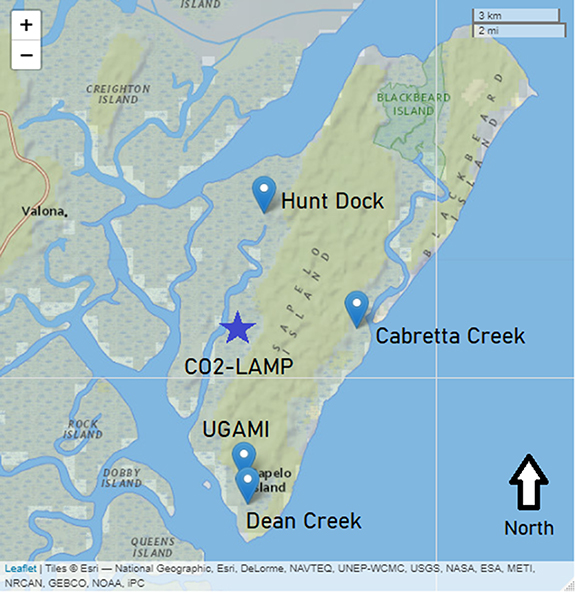
Figure 1. Map of instrument locations on Sapelo Island, created using 'leaflet' package in R. Background from Esri. UGAMI stands for University of Georgia Marine Institute. The star denotes the floating pCO2 sensor platform. Sapelo Island is located at 31.48 lat, 81.24 long. Map created using 'Leaflet' package in R (Cheng et al 2022). © 2014–2016 RStudio, Inc.
Download figure:
Standard image High-resolution image2.2. Tide data
Sapelo Island hydrography is characterized by a strong tide (Ragotzkie and Bryson 1955), which varied as much as 3.23 m during the study period at Hunt Dock. Tide height, water temperature, salinity, and turbidity were recorded by NOAA (National Oceanic and Atmospheric Administration) tide gages in 15 min intervals at three different locations: Hunt Dock, Cabretta Creek, and Dean Creek (figure 1; NOAA Tides & Currents 2021, NOAA NERRS 2022). The 15 min tide height, water temperature, salinity, and turbidity, and 1 h moon phase data were linearly interpolated to match exactly the pCO2 timestamps for the purpose of statistical testing. After interpolation, all data had a resolution of approximately 1 h. Tides lasted an average of 12 h, 25 min, and 15 s from high tide to high tide during the study period. Water temperature ranged from 27.2 °C to 33.4 °C at Hunt Dock during the study period. Geocentric moon phase data at hourly intervals in 2021 was retrieved from NASA Scientific Visualization Studio (Wright n.d.).
2.3. Flux data
Atmospheric CO2 concentration (ppm) was from the Georgia Coastal Ecosystems LTER Flux Tower (US-GCE) at 31.44 lat, −81.28 long. US-GCE is owned and maintained by the University of Georgia Marine Institute (UGAMI), located 5.5 km from US-GCE, at 31.40 lat, −81.28 long. It is a 10 m tall triangle tower installed on an elevated dock platform. CO2 is measured by an enclosed CO2 gas analyzer (CSAT LI7200) at 10 Hz frequency, then averaged to produce half-hourly data (Feagin et al 2020). Half-hourly data was used in this study due to less noise, then was linearly interpolated to exactly match pCO2 timestamps. The tower is accessed from UGAMI by car, boat, and then walk through the marsh.
2.4. Smart Rock
The Smart Rock is a low-cost submersible sensor developed by the OPEnS Lab (Openly Published Environmental Sensing Lab) and provided by the Consortium of Universities for the Advancement of Hydrologic Sciences, Inc. (∼$200). It measures turbidity and salinity but can also measure water level and temperature when in calibration mode (Veach 2019). Salinity was measured using the Gravity: Analog Total Dissolved Solids Sensor/Meter for Arduino manufactured by DF Robot, with a measurement range 0–1000 ppm (∼0–2000 uS cm−1) and accuracy within 10%. Turbidity was measured using the Gravity: Analog Turbidity Sensor for Arduino, also manufactured by DF Robot, with a measurement range of 0–4.5 V and accuracy within 0.3 V. Turbidity and salinity were recorded by the Smart Rock once every 20 min. Turbidity and salinity from both the Smart Rock and NOAA tide gage are presented in the results. However, only measurements from NOAA tide gages were used for analysis.
2.5. CO2-LAMP
The CO2-LAMP was deployed at the base of US-GCE. The CO2-LAMP measured pCO2 in both water and air in the tidal marsh. A waterproofed NDIR CO2 gas analyzer was used to measure pCO2. Data were logged using a CO2-LAMP recently developed by Blackstock et al (2019). In this platform, passive equilibration of dissolved CO2 in the water exchanges with a 'headspace' volume containing the CO2 gas analyzer enclosed by an expanded polytetrafluoroethylene (ePTFE) semi-permeable membrane. As previously reported by Johnson et al (2010), diffusion of CO2 in water primarily limits time needed for equilibration, but where runoff rapidly introduces water of dissimilar pCO2 values, passive equilibrators may not fully capture peak pCO2 values in some cases (Yoon et al 2016).
The NDIR gas analyzer used was a K30 10% manufactured by Senseair AB (Delbo, Sweden). The K30 10% manufacturer reported accuracy is ±300 ppm with a resolution of 10 ppm CO2 and capability of measuring up to 100 000 ppm. Prior to deployment, reference measurements were made using 0 ppm CO2 (99% N2, O2-balance) and 2000 ± 40 ppm CO2 (N2 balance) reference gases. After deployment, reference measurements were remade using a 0 ppm CO2 (N2) and 550 ± 2 ppm CO2. During reference measurements, the reference gas exchanges across the semi-permeable ePTFE surface and is measured by the K30 until equilibration is reached. Pre-deployment 0 ppm CO2 reference gas measurements were measured as 0 ppm CO2 by the K30, and the 2000 ppm CO2 reference measurements were measured as 1980 ppm CO2, which were within K30 analytical and reference gas concentration uncertainty. Post-deployment 0 ppm CO2 reference gas measurements were measured as 0 ppm CO2 by the K30, and the 550 ppm CO2 reference measurements were measured as 530 ppm CO2, indicating a consistent, slight underestimation (20 ppm) of gas concentrations and negligible drift relative to the range of the gas analyzer and previous ranges observed in surface waters at Sapelo Island (Wang and Cai 2004).
CO2-LAMP data were recorded every 10 s for 20 min, followed by 45 min of sleep. All measurements except the last measurement from each measurement cycle were removed during post-processing, resulting in approximately 22 datapoints per day with a resolution of 1.09 h each and 589 datapoints overall. Due to the unique CO2-LAMP measurement frequency, 15 min tide data, 30 min flux data, and hourly moon phase included in our analysis were interpolated to match the temporal resolution of pCO2. Values of pCO2 less than or equal to 0 ppm occurred infrequently during measurement cycles but were marked as non-physical values and replaced with the value of the previous measurement. Multiple sensors are preferred to compare pCO2 data, check for drift, and determine the degree of spatial variability. However, power limitations restricted simultaneous deployment of multiple CO2-LAMPs.
Another issue which impacted data collection was biological fouling, which is common when monitoring in coastal or other aquatic ecosystems. Minimum daily pCO2 measurements determined by the 22-point moving minimum linearly increased throughout the study, likely due to accumulation of biofilms and algae over the CO2-LAMP semi-permeable membrane (figure 2). Original data were detrended by fitting the daily moving minimum pCO2 to a simple linear regression. Fitted data was then subtracted from the original data, and atmospheric background CO2 of 420 ppm was added back in.

Figure 2. Original and detrended daily moving minimum pCO2 with respective linear best fit lines and their equations. The number of the observation is represented by n.
Download figure:
Standard image High-resolution imageThe CO2-LAMP was attached to a foam board capable of varying with tide height. This deployment was based on a similar, unpublished design by Thomas L O'Halloran at Clemson University (personal communication). The CO2-LAMP protective housing was attached to a foam swimming board' using marine epoxy and an extra-large zip tie to keep it elevated at the water surface with the waterproofed gas analyzer submerged below the water surface (figure 3). Because pCO2 concentrations at the air–water interface are most important to wind-driven gas exchange (Wanninkhof 2014), and pCO2 can vary within the water column (Beaubien et al 2014), consistent depth of measurement near the water surface is important. The bottom baseboard was held down with four t-shaped PVC pipes with holes drilled into the piping for drainage, which prevented the pipes from moving upwards over time. The top baseboard, sized 60.96 × 60.96 × 0.635 cm, was secured to the flux tower with zip ties threaded through holes in the wood and decking. Metal flanges with male adapter fittings were screwed into the top and bottom boards with wood screws. Three hollow five-foot copper pipes were then easily placed inside the adapter fittings on both ends and pressed or hammered down, with no further seal necessary. Only metal flanges and adapters can be used because the allowances fit with copper piping. Plastic pipe fittings did not fit with the metal pipes or flanges, though transition adapters could work in the future.

Figure 3. Schematic of CO2-LAMP tide-varying station, with height, width, and thickness dimensions. Blue lines represent hollow copper pipes held in place by metal flanges and adapters on the wooden top and baseboards. The black power line connects to a solar power array. The yellow waterproof sensor housing case is zip-tied onto the pink flotation device. (A) The sensor platform sits near the marsh surface at low tide, while the K30 sensor (white square) measures pCO2 in air. (B) The sensor platform floats upwards with the change in water level at high tide, measuring pCO2 just below the water surface. The dark blue square represents marsh surface water.
Download figure:
Standard image High-resolution imageLateral C export is referred to as a 'potential' throughout this study because it is solely based on contributions from pCO2 and does not account for the import or export of other forms of C. Tide velocity was calculated as change in tide height divided by change in time between pCO2 measurements. Atmospheric CO2 (ppm) measured at the flux tower was subtracted from pCO2 prior to the potential tidal C export estimation (table 1) and linear regression (figure 5) to eliminate any measurements potentially taken in air. Any measurements below zero after this correction were set to zero. Lateral import was assumed to occur when tide was increasing, and export when tide was decreasing. Cumulative imported and exported C were calculated for each tide cycle. Cumulative tidal imports were subtracted from cumulative tidal exports to achieve net export (gC m−2 s−1). Net export was then multiplied by the length of each tidal cycle in seconds and averaged to find the potential average C export per tidal cycle. Net export in seconds was also summed across the duration of the study to find potential total C export for the entire study. The equation used for calculations was:

Table 1. Tide gage locations and distances and potential tidal and total export of pCO2. Letters represent (A) Monte Carlo style estimate to account for sensor inaccuracies (B) actual observations assuming 100% sensor accuracy.
| Station | Lat. | Long. | Dist. (km) | Potential tidal export (gC m−2 tide cycle−1) | Potential total export (gC m−2 study period−1) | ||
|---|---|---|---|---|---|---|---|
| A | B | A | B | ||||
| Hunt Dock | 31.48 | −82.17 | 4.15 | 0.07–0.22 | 0.06 | 3.68–11.67 | 3.02 |
| Cabretta Creek | 31.44 | −81.24 | 4.15 | 0.03–0.16 | 0.04 | 1.62–8.47 | 2.25 |
| Dean Creek | 31.39 | −81.28 | 6.02 | 0.04–0.11 | 0.03 | 2.04–5.85 | 1.71 |
ρair was assumed to be 1225 g m−3. About 106 is the conversion factor for pCO2 (ppm).
2.6. Hypothesis testing
Vector autoregression and Granger causality were the selected methods for hypothesis testing. These methods work together and are ideal for complex datasets with multiple predictors. Vector autoregressive models are stationary, multivariate time series models which can be used to describe random stochastic processes with limited prior knowledge of the forces influencing each variable. One equation is created for each dependent variable using a linear function of the lagged dependent variable and other information. Akaike information criterion (AIC) of each model is calculated from the number of predictor variables and model performance. The best-fit model according to the AIC is then used in the Granger causality test.
The Granger causality test works well to examine underlying relationships in a dataset which the vector autoregression cannot. Granger causality originated in econometrics, but has since been adopted by many other fields, including the geosciences (Granger 1969, Detto et al 2012, Desai 2014). Granger causality should only be computed on stationary, modeled data rather than original or nonstationary data, and cannot be computed for singular matrices made of multiple, strongly interdependent variables. This model-test combination is a computationally simple way of assessing temporal relationships between variables. Some disadvantages of Granger causality testing are that results may be skewed by infrequent sampling, too-frequent sampling, nonlinear causal relationships, and more. Interpretations of Granger causality testing should align with the physical dynamics of a system, and not be used as stand-alone statistical results due to these limitations.
Hourly moon phase and 15 min tide height, salinity, turbidity, and water temperature were linearly interpolated to match pCO2 measurement times, which had a resolution of 1.09 h, for statistical testing. Moon phase was eliminated from statistical testing because it created a singular matrix due to its close relationship with tide height. The vector autoregression model was fitted to the dataset including tide height, salinity, turbidity, and pCO2 with lags ranging from 1 to 5. Model estimation was initialized using the first six observations as pre-sample data. The model with the best fit, according to the lowest AIC, was then used in the Granger causality test. To evaluate the accuracy of the vector autoregression model fit, half of the data (even-numbered observations) were withheld from the fitting procedure and pCO2 was estimated from the fitted model. The ability of the fitted model to predict the withheld values was then assessed using correlation and significance between pCO2 predictions and observations. Adjusted R2 of modeled tide height, salinity, turbidity, and pCO2 was also calculated. Lastly, model consistency and autopower spectral densities of the vector autoregression were reported. Model consistency measures the proportion of the correlation structure in both the observed and modeled data. Autopower spectra can be used to determine overlapping peak frequencies between observed and modeled data.
The leave-one-out Granger causality test was performed using the multivariate Granger causality toolbox in MATLAB, which assesses whether each variable in a best-fit vector autoregression model forecasts another variable (Barnett and Seth 2014). Results of the Granger causality test are described using p-values of each Granger causality and causal density, which is the average of Granger causalities between each pair of variables in a dataset with respect to the variables not included in each pairwise causality test. Datasets composed of variables that behave relatively independently will have higher causal densities because their predictors produce unique and useful information. Datasets with completely unrelated variables will have scores closer to zero, as the dynamics guiding each variable are different (Seth et al 2011).
2.7. Uncertainty analysis
To estimate the uncertainty of our approach, we constructed 100 pCO2 alternative timeseries datasets using a Monte Carlo style approach. The 100 datasets were created by randomly selecting numbers in the range of the original measurement ±300 ppm, to account for sensor accuracy. The potential tidal export was then recalculated using the simulated datasets to produce estimated upper and lower limits of tidal exports from the marsh.
3. Results
3.1. Tidal influence
The twice daily, or semidiurnal, tide at Sapelo Island had a clear influence on pCO2 (figure 4(A)). Tide also influenced changes in salinity and turbidity (figures 4(B) and (C)). Tide height at Hunt Dock reached a maximum of 4.5 m during the study (figure 4(D)). Water temperature was not strongly correlated with pCO2 (R = −0.09, p = 0.02). Surface water salinity as electrical conductivity surpassed the maximum limit of the Smart Rock sensor. Salinity peaks lined up well with peaks in tide height. Low tide was reflected in pCO2 measurements and tide height, but not by the salinity sensor. Salinity and pCO2 were also poorly aligned from 31 July to 3 August when both dropped to low levels. Relative turbidity indicated murky water was consistently brought in by the tide, and was especially murky on 25–27 July, and 21 August. Relative turbidity continued to decrease throughout the study, which means that surface water got darker with time.

Figure 4. Time series at Sapelo Island Marsh. (A) Observed pCO2 concentrations in ppm (yellow line) and modeled by vector autoregression (black dots). (B) Salinity measured by the Smart Rock and at Hunt Dock (uS/cm). (C) Relative turbidity measured by the Smart Rock (Volts) on the left axis and turbidity (nephelometric turbidity unit, NTU) at Hunt Dock on the right axis. Only turbidity less than 50 NTU is shown. Higher NTU indicates murkier water, while higher voltage implies clearer water. (D) Tide height at Hunt Dock (meters) and moon phase divided by 25 on the left axis and water temperature (°C) on the right axis.
Download figure:
Standard image High-resolution imageValues of pCO2 ranged from 390 to 6106 ppm ± 54 (standard error), with a mean of 1421 ppm. This equated to a range of 0–5596 ppm throughout the study period after accounting for atmospheric CO2, with a mean of 1081 ppm (0 standard error). There was a positive linear relationship (R2 = 0.35) between mean tide height and median binned pCO2 (figure 5). Most outliers, having pCO2 values greater than 1.5 times the interquartile range, occurred at tide heights below 3 m.

Figure 5. Box chart of pCO2 (ppm) according to tide height at Hunt Dock (blue boxes) with linear equation fitted to median pCO2 of each bin (black line). pCO2 was binned every 0.2 meters of tide height. The mean tide height for each bin, rounded to the nearest tenth of a meter, is displayed on the x-axis. Horizontal bars represent median pCO2 for each bin. The top and bottom of each box represent the upper and lower quartile. The whisker extending from each box represents minimum and maximum values. Outliers are shown as blue circles. Only pCO2 concentrations above 0 ppm after subtracting atmospheric CO2 are shown.
Download figure:
Standard image High-resolution image3.2. Net tidal C export and uncertainty analysis
Mean pCO2 during incoming tide was roughly half of mean pCO2 during outgoing tide, with an average concentration of 492 ppm compared to 1569 ppm after accounting for atmospheric CO2. This resulted in a potential net lateral C export of 0.03–0.06 gC m−2 tide cycle−1 and 1.71–3.02 gC m−2 during the entire study period as pCO2 at all tide gages, assuming 100% sensor accuracy (table 1). Potential tidal C export was largest when using Hunt Dock tide data. Potential lateral net C exports per tide cycle based on tide gages at Cabretta Creek and Dean Creek were similar despite different distances from the CO2-LAMP when 100% sensor accuracy was assumed.
Flow out of the marsh was highly variable dependent on sensor accuracy. Potential lateral net C export estimated using Hunt Dock tide data was 3.20 gC m−2 higher than estimations based on tide data at Cabretta Creek and 5.82 gC m−2 higher than estimations based on tide data at Dean Creek when summed across the entire study period according to the Monte Carlo style simulation. Although the range produced by the upper and lower bounds of the Monte Carlo style simulations for each tide gage were relatively small on average per tide cycle (range of 0.12 gC m−2 tide cycle−1), these led to large uncertainties in total C export for the study period overall (average range of 6.22 gC m−2 study period−1). Lower bounds of the Monte Carlo style estimates were similar to observations, but upper bounds were at least two times greater than observations across all tide gages.
3.3. Vector autoregression and Granger causality testing
The vector autoregression model explained 98% of the variation in tide height, 96% of the variation in salinity, 97% of the variation in water temperature, and 58% of the variation in pCO2 when considering the number of independent variables. The model results did not fit well with observations of turbidity, with an adjusted R2 value of −0.28. Model consistency was low at only 5%. Strong peaks in the autopower spectra for tide height and pCO2 corresponded with the frequency of the semidiurnal tide at roughly 2.3 × 10⁻⁵ Hz (figures 6(A) and (D)). A similar but weaker maximum frequency was observed in the autopower spectra for salinity (figure 6(B)). Turbidity reflected maximum autopower at the semidiurnal frequency for modeled data but not for observed data (figure 6(C)). Vector autoregression predictions of pCO2 aligned well with observations when withholding half of the data (R = 0.84) and when using the full dataset to fit the model (R = 0.83).

Figure 6. Autopower spectral densities from the vector autoregression model and time series data of (A) tide height, (B) salinity, (C) turbidity, (D) water temperature (°C), and (E) pCO2. Autopower is displayed on the y-axis and has units of the representative variable squared over Hz (e.g. m2Hz−1 for tide height).
Download figure:
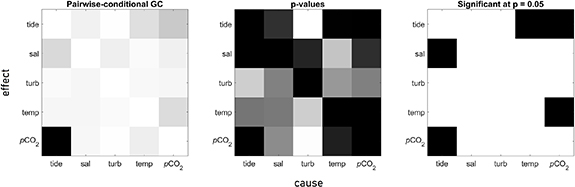
Standard image High-resolution imageGranger causality testing of the vector autoregression model using Hunt Dock tide data revealed causal relationships between tide height and water temperature, water temperature and pCO2, tide height and pCO2, and tide height and salinity (figure 7). Causal relationship direction (e.g. pCO2 –> tide ht.) was the opposite of reality in some cases. Mean causal density was 0.03.
Figure 7. Granger causality test results. (A) Pairwise-conditional Granger causalities, with darker squares representing higher values. Granger causality units are arbitrary. (B) Corresponding p-values for each pairwise Granger causality test, with darker squares representing lower, more significant p-values. (C) Significant Granger causalities only, with dark squares representing causal relationships. In all subplots, columns represent causes; rows represent effects.
Download figure:
Standard image High-resolution image
4. Discussion
4.1. Reliability of the CO2-LAMP
We demonstrated that the CO2-LAMP could measure the influence of tides on dissolved CO2 in a tidal marsh using a low-cost platform ($346–497 in 2022). Uncertainty in pCO2 measurements due to sensor accuracy using the manufacturer-provided ranges had a large influence over potential net export, in addition to atmospheric CO2 concentration and tide gage location. Nevertheless, it is important to note that the manufacturer-provided analytical error represents a maximum. Reference measurements inform that actual field measurements are likely much more accurate than the manufacturer-stated accuracy. A more thorough set of reference measurements would provide better statistics regarding individual sensor accuracy, which could then be used for refining the parameterization of the Monte Carlo style analysis. We assume the estimated uncertainty would be much lower in this case.
4.2. Cost and improvements of pCO2 and Smart Rock sensors
Large ranges in lateral flow estimates demonstrated difficulty with comprehensive measurement of water flow and the importance of co-located tide gages when measuring pCO2. When using water flow outside of the marsh to understand lateral C imports or exports from the marsh, overland and groundwater flow corrections should be made (Wang et al 2016), though such information was not available in this study. Overland flow is when water follows a path through the marsh not captured by a tide gage. More spatiotemporally frequent measurements of water flow are essential. One way to do this could be to use a fixed acoustic Doppler current profiler or measure particle tracking velocity using video, though video may be difficult in the marsh as wind effects on apparent surface water flow can lead to erroneous flow estimations.
Despite challenges faced with maintenance and operation, the CO2-LAMP performed well in detecting tidal export of C as pCO2. The sensor platform is simple to operate, lightweight, low-cost, and captures moderately frequent measurements necessary to understand influence of a full tidal cycle on marsh biogeochemistry. Mismatched peaks in salinity and pCO2 indicated there was likely residual moisture with relatively high salinity still on the sensor between some tidal cycles. Decreasing turbidity and pCO2 drift could have been caused by fouling on sensor surfaces or increased inputs of DIC from terrestrial freshwaters. Data from nearby streams from smaller catchments would be needed to validate this claim. Additionally, more frequent cleaning may resolve this issue. In future versions of the Smart Rock, the upper limit of the salinity sensor should be increased. Adding higher quality internal clocks to both the Smart Rock and CO2-LAMP will provide more reliable timestamps. Decreasing the power draw of the CO2-LAMP would also enable simultaneous data collection by multiple sensors at stations having smaller solar arrays.
The cost of the CO2-LAMP in 2022 ranges $346–497 with an added $180 minimum for the tide-varying station (i.e. wooden boards, copper pipes, etc), plus shipping and tax. Prices can change with individual product choices (e.g. type of K30, size of waterproof case), access to construction tools or lab supplies, and the number of supplies bought in bulk or reused. An itemized list of parts and costs are included in SI1. The CO2-LAMP uses the same measurement method as other low-cost pCO2 sensor platforms such as the SIPCO2, which had a cost of $500 USD in 2017 (Hunt et al 2017). A smaller, lower-cost, and submersible pCO2 sensor platform was developed by Hill (2018) for approximately $305 USD, though battery life was shorter. At its current price, the CO2-LAMP is still less costly than some other alternatives (Li 2022). The Smart Rock had a low cost of around $200 but was built most easily while taking an online course workshop, which adds to the overall cost. However, the internal battery and long-lasting low-power mode make the Smart Rock simple to use and implement.
4.3. Vector autoregression and Granger causality testing
The autoregression model demonstrated that variations in observations of turbidity are difficult to explain with this suite of variables, and the tidal influence on modeled salinity and turbidity are present, but weak. Neither modeled nor observed water temperature demonstrated a tidal signal. Granger causality testing revealed that although pCO2, turbidity, salinity, and water temperature fluctuated with tide height, any correlation between pCO2 and salinity is likely due to the influence of tide height on salinity. Causal density and vector autoregression model consistency were low. Low model consistency in this case could be the result of a missing key variable, such as tide direction. Nonzero causal density indicates that there was some dynamical complexity, but higher causal density might be achieved with more variables or a higher frequency and duration dataset, which would enable a greater lag capability and higher confidence in results. Alternative statistical techniques such as multiple linear regression may be better suited to describing tidal data in cases where the dataset is highly interdependent, or singular. Granger causality testing did not accurately predict the direction of some relationships potentially due to edge effects from overlapping signals, or distance between the tide gage and pCO2 sensor. More specifically, a sine wave of pCO2 may be viewed as 90° ahead of a sine wave of water temperature or 270° behind.
Our modeling approach could be used to increase spatial estimations of C imports and exports in salt marshes given certain assumptions. With an adequate training set and validation data collected through time, C imports and exports could be estimated. Investigators could expand C exchange monitoring using instrumentation like the CO2-LAMP to develop regression-based models where tide height and other water quality parameters are monitored. Intermittent CO2-LAMP (or similar system) deployments at potential sites would allow validation of the regression-based model and re-evaluation of model coefficients over time should cyclical or long-term changes be present in response to C exchange dynamics.
4.4. Tidal effects in coastal marshes
Fluctuation of pCO2 with the tide supported other studies which show tidal amplitude is a key variable in porewater discharge (Bouillon et al 2008, Maher et al 2013, Linto et al 2014, Call et al 2015, Seyfferth et al 2020) and groundwater discharge (Wang and Cai 2004, Tamborski et al 2021). Porewater and groundwater also contribute to lateral export of dissolved inorganic C, which includes CO2, bicarbonate (HCO3 −), carbonate (CO3 −), and carbonic acid (H2CO3). As a result, low tides may result in higher concentrations of CO2 partial pressure (pCO2) in surface water than high tides at some sites as high pCO2 porewater and groundwater become more dominant (Zablocki et al 2011, Burgos et al 2018, Taillardat et al 2018, Mayen 2020), especially during periods of low flow (Marescaux et al 2018). There was no strong evidence for that relationship in bin-averaged pCO2 and tide height in the marsh, though most pCO2 outliers existed at low tide heights. The marsh surface was also exposed during low tide, leading to a lack of underwater pCO2 measurements during low tide to compare with high tide. Tidal oscillation of pCO2 at Sapelo contrasted with coastal ecosystems of the English Channel, which have a much stronger diurnal variability despite a semidiurnal tide (Yang et al 2019). Measurements of groundwater and surface water flow from within the marsh were a limitation of this study but are crucial for understanding coastal C dynamics.
Potential net tidal export based on tide velocity at all stations was expected, as tidal marshes typically export more C than they import through lateral flow. A salt marsh in North Carolina demonstrated summertime lateral dissolved inorganic C export of approximately 0.5 gC m−2 tidal cycle−1, which was larger but similar in magnitude to the upper limits of C export based on tide velocity at Hunt Dock and Dean Creek using the Monte Carlo style simulation (Czapla et al 2020). Potential net C export for the entire month of study was lower than dissolved inorganic C export of more than 30 gC m−2 for the month of July in a Massachusetts salt marsh in all cases (Wang et al 2016). The cumulative annual C sink for the marsh in Sapelo ranges from approximately 130–300 gC m−2yr−1 (Nahrawi 2019) and can range from 380 to 890 gC m−2yr−1 in other subtropical marshes (Gomez-Casanovas et al 2020, Liu et al 2020). Total lateral C export during the month of study alone would account for approximately 0.5%–9% of the cumulative annual C sink of the marsh. The estimates presented here were based on measurements taken during the peak of the growing season when photosynthetic productivity and respiration rates are high, and they should not be extrapolated throughout the rest of the year. Granger causality of tide height means that small changes in tide height across the marsh surface could have a large impact on seasonal and long-term fluctuations in C export due to pCO2.
Additionally, subtropical salt marshes can display 'hot' moments of high C export or import, such as the coastal marsh in Codden et al (2022) where as much as 12% of annual organic C sequestration was exported as DOC in one summer month across a 16 month study. Longer term monitoring would be necessary to determine whether our measurements reflect a 'hot' moment. Our lateral C export estimate likely underestimates actual lateral C export from the marsh because it does not consider the import or export of other forms of C, such as particulate organic C, dissolved organic C, or C in CH4. Subtropical coastal salt marshes such as Sapelo Island are among the most productive ecosystems on Earth and given high spatiotemporal variability of these types of measurements, continual monitoring is important.
A weak, positive linear relationship between marsh surface water pCO2 and tide height was in line with results from previous studies at this site. Specifically, aquatic pCO2 concentrations aligned well with previous measurements of ∼3250 and ∼2500 ppm during low tide and high tide, respectively in June 2001 at Barn Creek (Wang and Cai 2004). Maximum pCO2 concentrations were still lower than those of a tidal creek in Delaware, USA of around 8400 ppm (Trifunovic et al 2020). Surface water pCO2 aligned with the observations of ∼1086 ppm and ∼493ppm during low tide and high tide respectively at the mouth of Doboy Sound in June 2003, when accounting for atmospheric CO2 (Jiang et al 2008).
5. Conclusion
Here, we evaluated a low-cost pCO2 sensor platform at Sapelo Island, Georgia, USA as an approach to address the desire for more frequent and more extensive sampling of pCO2 in coastal marshes. We hypothesized that (a) CO2-LAMP measurements of pCO2 would support previous research findings that Sapelo Island marshes are a lateral C source, and (b) comparison of pCO2 measurements with tidal data would demonstrate known biogeochemical mechanisms, including positive correlations with turbidity and salinity, a weak inverse correlation with water temperature, and higher concentrations during ebb tide than flood tide.
In accordance with our first hypothesis, we found that the CO2-LAMP is an effective tool for studying aquatic biogeochemistry and capturing tidal signals using semi-frequent measurements. Results of pCO2 tidal variability demonstrated net lateral C export as pCO2 and higher pCO2 concentrations during outgoing tide (ebb) than incoming tide (flood), but some difficulties remain when teasing apart signal from complex tidal data.
Our second hypothesis was partially supported by Granger causality results showing that. Tide height was a significant driver of pCO2, salinity, and water temperature, although the direction of causality was incorrect. pCO2 had a weak inverse relationship with water temperature, a positive linear relationship with tide height, and was higher during outgoing tide (ebb) than incoming tide (flood).
As coastal wetlands begin to migrate landwards or disappear because of urbanization, topography, and rising seas, the pressure to understand and conserve them increases (Borchert et al 2018, Thorne et al 2018). Scientific collaboration and a clearer understanding of biogeochemistry in tidal ecosystems could contribute to better modeling of coastal environments influenced by hurricanes, sea-level rise, groundwater abstraction, and more (White and Kaplan 2017). In combination with other measurements, pCO2 can provide a window into the biogeochemistry of coastal ecosystems.
Acknowledgments
We would like to thank the dedicated team of researchers and field technicians at UGA and UGAMI, including Jacob Shalack, Peter Hawman, and Dr Deepak Mishra, and our reviewers for their valuable feedback. This work also benefitted from insights on Granger causality testing from Dr Paul Stoy and Dr Matteo Detto, and post-deployment lab testing by Jonathan Thom of the Space Science and Engineering Center at UW-Madison. This material is based upon work supported by the National Science Foundation Graduate Research Fellowship Program under Grant No. DGE-1747503. Any opinions, findings, and conclusions or recommendations expressed in this material are those of the authors and do not necessarily reflect the views of the National Science Foundation or the USDA. Any mention of commercial names or products does not imply USDA endorsement.
Data availability statements
The data that support the findings of this study are openly available at the following URL/DOI: 10.5281/zenodo.6403170. MATLAB scripts and datasets created for this research are available on GitHub (turner-j 2022) and through the Environmental Data Initiative (EDI) Data Portal (Turner 2022). Others can be found using the in-text citations (NOAA Tides & Currents 2021, NOAA National Estuarine Research Reserve System (NERRS) 2022). Flux data from US-GCE are available from the site Principal Investigators upon reasonable request using contact information on AmeriFlux.
Supplementary data (0.3 MB PDF)