


Abstract
Green ammonia has been proposed as a technologically viable solution to decarbonise global shipping, yet there are conflicting ambitions for where global production, transport and fuelling infrastructure will be located. Here, we develop a spatial modelling framework to quantify the cost-optimal fuel supply to decarbonise shipping in 2050 using green ammonia. We find that the demand for green ammonia by 2050 could be three to four times the current (grey) ammonia production, requiring major new investments in infrastructure. Our model predicts a regionalisation of supply, entailing a few large supply clusters that will serve regional demand centres, with limited long-distance shipping of green ammonia fuel. In this cost-efficient model, practically all green ammonia production is predicted to lie within 40° latitudes North/South. To facilitate this transformation, investments worth USD 2 trillion would be needed, half of which will be required in low- and middle-income countries.
Export citation and abstract BibTeX RIS

Original content from this work may be used under the terms of the Creative Commons Attribution 4.0 license. Any further distribution of this work must maintain attribution to the author(s) and the title of the work, journal citation and DOI.
1. Introduction
Maritime transport handles around 80% of global trade by volume [1], making it imperative for the global economy. However, maritime vessels currently run predominantly on cheap, energy-dense heavy fuel oils (HFOs), which is responsible for around 2.9% of global anthropogenic greenhouse gas (GHG) emissions [2]. In 2018, the International Maritime Organization (IMO) committed to decarbonize the sector, aiming to reduce GHG emissions by 50% in 2050 compared to the 2008 baseline, alongside a set of other regulatory actions [2]. More recently, calls have been made to set even more ambitious targets and completely decarbonise the sector by 2050 [3].
The shipping industry faces considerable hurdles to achieve the decarbonisation targets set, in particular given long asset lifetimes, the price gap between HFO and green fuel options, a large number of independent stakeholders which will need to coordinate (e.g. engine manufactures, ports, carriers, production facilities, investors) [4–7]. As such, there is considerable uncertainty in terms of the optimal path to decarbonise the maritime sector relating to the future energy fuel mix and the infrastructure necessary to facilitate this new fuel supply-chain [8–10].
Recently, the international community has converged on green ammonia (ammonia produced using renewable energy only) as a likely candidate in the long-run (i.e. mid to end-century) for long-haul maritime transport [7, 9, 11], given that (i) it is relatively energy dense (∼3.6 kWh L−1) compared to liquid hydrogen (∼2.3 kWh L−1) [12], (ii) it is easy to handle, as it is liquid under relatively mild conditions (it boils at −33 °C under atmospheric pressure), (iii) it can be produced in very large volumes (in the order of hundreds of million tonnes/annum) at low costs (between 10 and 100 USD/GJ) [13] and without competing for agricultural land (which is the drawback of biofuels), and (iv) several manufacturers have announced commercialisation of ammonia-fuelled maritime vessels by 2025–2030 [14]. According to a projections by several studies [9, 10], green ammonia could constitute 43%–99% of the shipping fuel mix in 2050, which would be equivalent to, or several times more than, the over 180 million tonne of ammonia produced globally at present (mainly for the fertilizer industry) [12]. Some environmental concerns relating to NOx emissions from ammonia engines remain, but these can be ameliorated using selective catalytic reduction and other advanced combustion techniques [13]. Overall, ammonia is a very likely candidate for the decarbonisation of shipping fuels, and more detailed techno-economic analysis is required to better compare it to other potential options.
Notwithstanding the technical and cost advantages of extensive use of green ammonia for shipping, the industry and investors currently lack credible scenarios for how a global green ammonia industry for shipping could be configured. This is partly driven by a limited understanding of where green ammonia could be most cost-efficiently produced in the future [13], and how to establish a fuel supply chain (spanning site selection, land transportation, processing, transportation to fuel demand centres) [12]. So far, studies investigating potential production locations of green ammonia for shipping have not adopted a rigorous techno-economic approach [7]. Where fine-scale estimates of site-specific (green) ammonia production have been developed [12, 13, 15], those spatially explicit production cost estimates often do not include fuel-supply costs and have not yet been extended to an analysis of global fuel supply-chains beyond a small number of routes [16]. Similarly, while one study estimated that cumulative capital costs to decarbonize the shipping industry by 2050 could be up to 1.9 USD trillion, of which 85%–90% would be fuel supply infrastructure (the remaining being cost related to energy efficiency technologies and ship engines) [10], it is not clear where this investment would be needed. Hence, major research gaps exist in terms of developing a geospatial global scale understanding of likely demand locations of future maritime fuels, taking changes in trade into consideration, and the optimal fuel supply network to meet this demand.
Here, we develop a port-level (1360 ports) fuel demand model for 2050 by scaling current fuel demand on transport routes with trade scenarios for 2050. We combine this with a spatially granular optimisation model of green ammonia production, storage, and transport on a global scale [12], finding the optimal production locations to meet demand for shipping fuel in 2050. We consider two future decarbonisation scenarios for 2050, a moderately ambitious (MOD-AMB) future scenario and highly ambitious (HIGH-AMB) future scenario, which include assumptions regarding future shipping trade (notably overall growth in trade and the quantity of fossil fuels that will be shipped in 2050), the levelised cost of ammonia production, and fleet adoption rate of ammonia-compatible maritime vessels (see table 1). The overarching model is schematised in supplementary figure 1.
Table 1. Overview of the two 2050 scenarios adopted throughout this study and key results. Note costs specified for energy and ammonia are averaged across the cases and are calculated individually at each location. See section 4 how these model assumptions are derived.
| Description | MOD-AMB | HIGH-AMB |
|---|---|---|
| Socio-economic growth | Shared Socioeconomic Pathway 'Middle of the Road' (SSP2) | Shared Socioeconomic Pathway 'Sustainability' (SSP1) |
| Decarbonisation | Representative Concentration Pathway 4.5 | Representative Concentration Pathway 2.6 |
| Fleet adoption rate | 70% | 90% |
| Levelised energy cost from solar PV with capacity factor = 20% | 14.4 USD/MWh | 10.7 USD/MWh |
| Levelised energy cost from onshore wind with capacity factor = 45% | 21.9 USD/MWh | 20.0 USD/MWh |
| Levelised ammonia production costs | 260 USD/tonne | 237 USD/tonne |
Our results provide the first comprehensive picture of supply and demand for the future green ammonia economy, which indicates an efficient future configuration of the global ammonia production and supply-chain network.
2. Results
2.1. Present and future fuel and green ammonia demand
Annual fuel demand is determined by the fuel consumption of maritime vessels, which can differ considerably between vessel types and size, the operating speed of vessels, and the distance travelled within a year [17, 18]. We estimate the fuel consumption and operating speed for 97 500 trade-carrying vessels (see section 4) and combine this with a dataset of port visits for each vessel for the year 2019 [19]. We aggregate the fuel consumption across port-to-port routes (between 1360 ports in our database, using real maritime distances), thereby deriving the fuel needed at the port of origin to reach the next port of call. We project the port-level fuel demand with the expected increase in port throughput for 2050 under two trade scenarios, which vary according to the socio-economic growth and decarbonisation scenario adopted (see table 1). This is done using present and future port throughput derived from the OxMarTrans model [1], a global maritime transport model that simulates the route allocation of maritime flows between countries (see section 4).
In total, we estimate global fuel consumption to be 233 million metric tonnes per annum (MMTPA) in 2019. This number is in line with the reported amount of global bunkering fuel for shipping by the IMO's Ship Fuel Oil Consumption Database [20], in which fuel consumption was estimated to be 213 million tonne in 2019. However, IMO's consumption estimate is based on reporting of 27 221 vessels (>5000 gross tonnage, which use the vast majority of fuel), compared to 97 500 vessels in our database. Our database also includes passenger and cruise ships (which contributes 3.5% to global fuel consumption). In supplementary table 1, we show the contribution of the different vessel types to global fuel demand, and in supplementary figure 2 we show the cumulative distribution of fuel demand over the distance travelled between ports in 2019.
HFO fuel demand (across all distances) is expected to increase to 434.0–446.2 MMTPA in 2050 given trade projections. Supplementary figure 3 shows a port-level disaggregation of the demand, which is achieved based on forecast trade projections, assuming ships bunker enough fuel at each port to carry the goods they collect to their destination—see the section 2 for more details. Using the fleet adoption rates adopted in table 1, combined with the equivalent energy efficiency of ammonia (1 tonne of HFO ≈ 2.07 tonne of ammonia), we project global demand for green ammonia fuel to be 601.5 MMTPA under the MOD-AMB scenario and 749.1 MMTPA under the HIGH-AMB scenario. Figures 1(a) and (b) shows the demand per country, after aggregating the demand on a port-level (supplementary figure 4 for port-level estimates). Large demand is predicted for prominent countries that depend on (long-distance) maritime transport, including the USA, Singapore, Japan, South-Korea, China, Brazil, India, Australia, South Africa, and Malaysia. These top 10 countries (out of 178 maritime countries) demand 57.0% (HIGH-AMB) and 58.2% (MOD-AMB) of the global green ammonia fuel.

Figure 1. Global green ammonia fuel demand by 2050. (a) Country-aggregated green ammonia demand under the MOD-AMB scenario. (b) Same as (a) but under the HIGH-AMB scenario. (c) Cumulative ammonia demand across ports. The horizontal lines indicate the ammonia required to meet the demand for the top 10, 50 and 100 ports. (d) Same as (c) but per region (in relative terms), with the horizontal line indicating the relative demand that can be met by targeting the top 10 fuel demanding ports.
Download figure:
Standard image High-resolution imageFigure 1(c) shows the global concentration of green ammonia fuel demand across the 1360 ports considered, showing large demand inequality. In other words, by targeting the largest ports first, a substantial amount of shipping can be decarbonised. For instance, targeting the top 10, 50, and 100 ports globally in terms of fuel demand (horizontal lines in figure 1(c)) would meet 21.3% (21.8%), 45.7% (46.7%), and 62.0% (62.6%) of the cumulative green ammonia fuel demand, respectively, under the MOD-AMB (HIGH-AMB) scenario. These port demand inequalities can be even larger regionally, as shown in figure 1(d), with the horizontal line showing the cumulative regional demand that can be met by targeting the top 10 ports. For instance, in Oceania, North Africa, South Asia and South-East Asia, over 60% of fuel demand can be met by targeting the top 10 regional ports as measured by fuel demand.
2.2. Levelised costs
We utilize a spatially-explicit green ammonia production model for 2050 [12], with ammonia production cost and capacity estimated on a 1 × 1 degree grid. This results in a dataset of 15 000 potential (wind and solar) supply locations on-land (see supplementary figure 5 for the spatial production cost estimates), of which we only consider the 4000 most likely locations for production based on cost and land availability (see Methods).
In both the MOD-AMB and HIGH-AMB scenario, the lowest production cost locations in 2050 predominantly rely on solar electricity (only ∼20% of production sites rely on wind with installed capacity of ∼1%). Although the capacity factor of solar (which is between 20%–30% for most locations at <40° latitude) is lower than the best wind sites, its installation cost are very low. Across these sites in both scenarios, there is potential for installation of 60 TW of solar PV dedicated to maritime fuel production, which translates to around 17 000 MMTPA of ammonia production capacity, around 25 times the ammonia demand in this model (despite the significant constraints imposed on land usage—see supplementary figure 6).
The levelised cost of ammonia supply (LCOA, in USD per tonne), which includes the production costs, electricity costs, pipeline construction cost, port storage (at the exporting and importing ports) and ocean transport, differs geographically (see figures 3(a) and (b)). Globally, the weighted average LCOA is 237 USD/tonne under the HIGH-AMB and 260 USD/tonne under the MOD-AMB scenario, which would be equivalent to an HFO cost of between 490 and 540 USD/tonnes (given the energy density difference), similar as the cost of very low sulphur fuel oil at present.
The cost breakdown per geographical demand region (figure 2) shows that production in North Africa has the lowest average (weighted) delivered LCOA, given almost no transport costs (mainly domestic production). Driven by the reduced production cost, all regions have a delivered LCOA in the HIGH-AMB scenario that is approximately 10% lower than the MOD-AMB scenario. The highest LCOA is for countries in Europe, which depend disproportionately on shipped imports, increasing the delivered LCOA. However, cost differences are relatively small across regions, driven by the relatively similar cost of producing green ammonia, which dominate the total LCOA (production and electricity cost is between 76% and 95% of LCOA across regions). The largest regional difference is only about 18% of the value of the fuel in both scenarios. In other words, all regions will have a similar LCOA to decarbonise the shipping sector long-term.

Figure 2. Regional variations in levelised cost of ammonia and cost breakdown. (a) The total LCOA across geographic demand regions under the MOD-AMB scenario, including the cost breakdown in six cost components (production, electricity, pipelines, supply storage, demand storage and ocean transport). (b) Same as (a) but under the HIGH-AMB scenario. The black markers indicate the total ammonia demand per region.
Download figure:
Standard image High-resolution image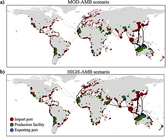
Figure 3. Optimal spatial fuel supply to meet global port fuel demand. (a) Cost-optimal fuel supply-chain under the MOD-AMB scenario, with green markers indicating production locations, blue markets fuel exporting ports, red markers fuel demand ports, and the lines the fuel shipments from exporting to demand ports. (b) Same as (a) but under the HIGH-AMB scenario.
Download figure:
Standard image High-resolution image2.3. Cost-optimal green ammonia fuel supply
A spatial representation of the optimal ammonia fuel-supply chain under both scenarios is shown in figure 3, showing the optimal production locations (green markers), port exports (blue markers) and port imports (red markers). Large production locations are shown in Northern and Western Australia, Chile, Western Africa, India, and the southern Arabian Peninsula. A clear 'regionalisation' of supply can be observed, where efficient production locations are paired with regional concentrations of demand, due to the costs associated with transporting ammonia over very long distances. Consequently, under both scenarios, maritime supply distances (i.e. distance from exporting port to importing port) are generally quite short; the average maritime distance travelled is around 4,800 kilometres, and only 0.03% of ammonia travels 10 000 km or more (the maritime distance from Middle East to Western Europe). In addition, because of the low cost of solar, production tends to be clustered relatively close to the equator; in both scenarios, less than 10% (2%) of ammonia is made at an absolute latitude greater than 30 (40) degrees. As a consequence of this, some regions produce very little ammonia themselves—Europe, for instance, consumes about 9% of ammonia demand in both scenarios, but produces less than 0.05% of the global supply.
Under the optimum fuel supply network, export markets are somewhat concentrated: out of the 1380 ports in 178 countries that demand fuel, only 30 ports in 11 countries export fuel in the MOD-AMB scenario, which rises to 32 ports in 14 countries in the HIGH-AMB scenario (supplementary figure 7). These exporting ports supply around 75% of the total ammonia demand in both scenarios, with the remaining ammonia being provided domestically by pipelines over land.
Australia is the most dominant provider of internationally exported green ammonia, providing almost 50% of the total exported ammonia in both scenarios, and almost four times as much as the second largest exporter, Chile. Interestingly, Australia ranks only as the 19th country out of all ammonia-producing nations in terms of production cost, with production cost almost 10% more than the cheapest exporting country (Argentina). What drives Australia's export potential is the relatively short shipping distance from Australia to Asian demand hubs (∼50% of fuel demand), and its significant amounts of available land, which allows scaling-up of ammonia supply. In other words, while being a second-best supplier in cost terms, the vast scalability of ammonia production makes it the most important global supplier of green ammonia fuel.
2.4. Global investment needs
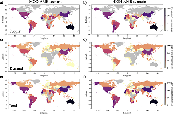
Figure 4 shows the country-aggregated investment needs on the supply-side (i.e. production, electricity, pipelines, storage at exporting port), figures 4(a) and (b) and the demand-side (i.e. storage at importing port and maritime transport costs), figures 4(c) and (d), and the combined investment need (figures 4(e) and (f)). On a global scale, we estimate the total investment need to be between USD 1.98 trillion (MOD-AMB) and USD 2.25 trillion (HIGH-AMB). Despite the fact that 25% more ammonia is being consumed under the HIGH-AMB scenario, total investment costs are 13% higher, underlining the benefits of accelerated progression down the renewable technology cost curves associated with more ambitious climate policies (table 1). Out of the total investment need, 8% is on the demand-side, while the remaining 92% is on the supply-side. Investment in the order of USD 2 trillion is in line with other estimates [10] that quantified global investment needs on the supply-side only to be USD 1.9 trillion, which additionally included the retrofitting costs of ship engines (10%–15% of estimated investment needs), but excluded electricity costs.
Figure 4. Global supply and demand-side investment needs. (a), (b) Total supply-side (production, electricity, pipelines and supply storage costs) investment need across countries under the MOD-AMB (a) and HIGH-AMB (b) scenario. (c), (d) Total demand-side (demand storage and oceans transport costs) investment need across countries under the MOD-AMB (c) and HIGH-AMB (d) scenario. (e), (f) Total investment need (supply and demand-side) across countries under the MOD-AMB (e) and HIGH-AMB (g) scenario.
Download figure:
Standard image High-resolution image
Large supply-side investments are required in Australia, Morocco, Mauritania, and Oman, while demand-side investments are required in China, the United States, Brazil and India. Altogether, green ammonia as a maritime fuel will significantly shift the spatial pattern of the maritime fuel supply chain compared to the existing fuel supply network of HFO (which is concentrated in oil-producing countries). For instance, of the total global investment needed, half of it would be needed to build infrastructure in lower- and middle-income countries.
3. Discussion
Shipping is one of the most challenging sectors to decarbonize because of the need for fuel with high energy density and the difficulty of coordinating maritime actors to produce, utilize and finance alternative (green) fuel supply. One of the main obstacles has been deep uncertainty in how this coupled system of fuel supply, trade and shipping fleet may evolve in the future. In this paper, we have provided two scenarios of the most cost-efficient global arrangements for green ammonia production and supply to fuel a decarbonised shipping fleet. This should help to create greater clarity amongst investors (in ammonia production, transport, bunkering and ships) of how the global system may look in 2050.
The implications are striking. Current dependence upon oil-producing nations, with crude oil being shipped very long distances and being separated into HFO nearer to demand hubs, is likely to be replaced by a more regionalised industry; green ammonia will be produced near the equator in countries with high solar potential and abundant land, and shipped to regional centres of shipping fuel demand. The greatest investment need, and opportunity, is in Northern and Western Australia, which is projected to become the main supplier for Asian markets. Large production clusters are also predicted in Chile (to meet demand in South America), California (to meet demand in Western U.S.A.), North-West Africa (to meet European demand), and southern Arabian Peninsula (to meet local demand and parts of south Asia). At present, our model optimises for the global minimum delivered cost of green fuel. Further research should consider features other than cost which may drive selection of production locations, such as fuel security, although for the globalised maritime industry, cost is a very strong driver.
We find that green ammonia production could reach up to 602 MMTPA under the MOD-AMB scenario and 750 MMTPA under the HIGH-AMB scenario, equivalent to a three to four-fold increase of present-day production of fossil fuel-based ammonia. While one of the benefits of ammonia compared to other potential fuels is the existence of a global market for the product [21], a considerable scaling up is required to meet the rising demand for ammonia in the future. As such, there are uncertainties regarding to what extent the market for (green) ammonia could be scaled-up, and how the market would be organised [22]. However, we also find that the majority of fuel demand will be needed at a relatively small number of ports, illustrating that the transition to ammonia fuelled shipping could begin at a small number of strategic ports that could become 'green shipping corridors', which are routes between two or more ports that will be prioritised for decarbonisation [23]. Targeting the top 10 fuel demanding ports globally could meet 21% of global fuel demand, but regional targeting strategies could meet >60% of fuel demand by targeting the top 10 regional fuel demanding ports only.
Decarbonisation of the global shipping industry will take place at the same time as fossil fuels are largely removed from global energy systems, lowering demand for maritime transport (energy products account for ∼36% of global maritime trade in 2021 [24]). Meanwhile, ammonia production for fertilizers will transition to green ammonia, whilst there may be significant uses of ammonia for energy storage. These other uses of ammonia have not been included in our optimisation, which may modify somewhat the global pattern of ammonia production, though the locations that are efficient for producing ammonia for shipping will also be favourable to supply future agricultural and energy markets. In particular, given existing land constraints in the model, places such as Australia (with moderately low production costs, but large land availability) would become even more important as suppliers of green ammonia.
The global average levelised costs of ammonia supply are predicted to be 237 USD/tonne under the HIGH-AMB and 260 USD/tonne under the MOD-AMB scenario, with remarkably small regional differences in LCOA (within ∼20%, see figure 2), driven by the large cost convergence and availability of solar energy globally, and the dominance of production costs in LCOA. In contrast, at present, there are stark differences in regional green ammonia production costs [25]. This raises important questions how to best decarbonize the maritime sector using green ammonia in the time frame between ∼2025 (expected timeframe of first ammonia-fuelled engines) and 2050. For instance, proposed wind-based projects in Europe, or developments in the US supported by the Inflation Reduction Act may shift the regional production costs. In other words, this work demonstrates that such initiatives would not be the long-term cost optimum, and therefore provides a scenario against which deviations from the cost optimum can be measured.
We find investment needs to transition to a green ammonia fuel supply chain by 2050 to be around USD 2 trillion, the vast majority of which would be needed to finance supply infrastructure. Consideration of other constraints such as fuel security may drive investment needs higher. Of this total investment need, half of it would be needed in low and middle income countries, which provides opportunities for foreign investments and green jobs, as previously identified [7]. However, at present, cost of capital is often higher in low and lower middle income countries, which could place a barrier on the flow of finance to construct renewable energy projects, such as green ammonia production [26]. Therefore, an enabling environment, in terms of investment security, skills, and governance, needs to be established such that the future green ammonia market can contribute to a green transition of developing economies.
4. Methods
4.1. Overview
The purpose of this work is to integrate a number of models, each of which provides a key piece of information relating to the decarbonised maritime industry in 2050. An overview representation of the models is provided in supplementary figure 1.
4.2. Maritime decarbonisation scenarios
We construct two plausible future maritime decarbonisation scenarios for 2050, which vary according to the degree of ambition to decarbonise shipping, the levelised cost of (green) ammonia (LCOA) production, and the composition and magnitude of global trade. The latter determines the demand for maritime transport, and which ports will likely be used to meet this demand. An overview of the two scenarios is shown in table 1, including a description of the different assumptions made. The MOD-AMB scenario assumes that the global economy, and hence maritime trade, will evolve in line with RCP4.5-SSP2, that 70% of the vessel fleet will be converted to green ammonia vessels, and uses renewable energy cost forecasting information for LCOA estimation that causes a moderate reduction in ammonia production cost (see Green ammonia production subsection). The HIGH-AMB scenario assumes that maritime trade will evolve in line with RCP2.6-SSP1, that 90% of the vessel fleet will be converted to green ammonia compatible vessels, and assumes a steeper reduction of the LCOA (see Green ammonia production subsection).
4.3. Vessel fuel consumption
The fuel consumption of a vessel is mainly determined by the vessel characteristics (vessel dimensions and carrying capacity, operational speed, power of engines) [17, 18]. To obtain insights into global fuel consumption, we utilize empirical vessel movement information for around 97 500 maritime vessels (see 'Transport and fuel demand model' subsection). For each vessel, we predict its fuel consumption per kilometre travelled.
We start by estimating a vessel-specific fuel consumption rate using a vessel-type specific linear regression. Regression formulations are well established for predicting vessel fuel consumption [17]. We use daily fuel consumption (FC), in tonne per day, as predictive variable and vessel carrying capacity (deadweight tonnage, DWT), installed horsepower of main engines (P), and operational speed (V) as explanatory variables. We fit separate regression models for different vessel types (v) to capture type-specific relationships. This regression model can be written as:

with  the error term and
  i
the regression coefficients. To fit the regression models, we use a database provided by IHS Markit, which contains the necessary information for around 19 000 maritime vessels. An overview of the vessel types is provided in supplementary table 1. The fit of the model is good, with R2 values between 0.93–0.98. Using these regression formulas, we can predict fuel consumption for 41 600 vessels (out of the 97 500) that have information provided in the IHS-Markit vessel database. For the remaining vessels, we set-up a regression based on DWT alone, and predict values of V and P based on DWT. Despite the simplicity of this regression model formulation, the R2 values are still between 0.54–0.86 (see supplementary table 1). We translate the daily fuel consumption to fuel consumption per travelled kilometre (tonne per km) by dividing the FC with the V of the vessel travelled. We end up with a database of vessel fuel consumption for 97 500 maritime vessels.
i
the regression coefficients. To fit the regression models, we use a database provided by IHS Markit, which contains the necessary information for around 19 000 maritime vessels. An overview of the vessel types is provided in supplementary table 1. The fit of the model is good, with R2 values between 0.93–0.98. Using these regression formulas, we can predict fuel consumption for 41 600 vessels (out of the 97 500) that have information provided in the IHS-Markit vessel database. For the remaining vessels, we set-up a regression based on DWT alone, and predict values of V and P based on DWT. Despite the simplicity of this regression model formulation, the R2 values are still between 0.54–0.86 (see supplementary table 1). We translate the daily fuel consumption to fuel consumption per travelled kilometre (tonne per km) by dividing the FC with the V of the vessel travelled. We end up with a database of vessel fuel consumption for 97 500 maritime vessels.
4.4. Transport and fuel demand model
Fuel demand at any given location, in this case at the port-level, is determined by the number of vessels calling at a port, their journey length (distance travelled), and the fuel consumption of vessels.
We obtained empirical vessel movement data, using Automatic Identification System data, for 97 500 vessels for the year 2019. Using this information, we have constructed a dataset of port-to-port visits of every vessel, covering 1380 ports in total, including the distance between ports. More information about this dataset is provided in previous work [1, 19]. Combined with the vessel fuel consumption database, we estimate the fuel need on every route (multiplying fuel consumption per km with the route distance). Global fuel demand per port is derived by assigning all fuel consumption of outgoing vessels to the port of origin. In other words, we assume that all vessels leaving a port will get their bunkering fuel from the port they just visited before starting their journey to the next port of call. Although a simplistic assumption, this allows us to project present-day fuel demand into the future (see 'Future fuel demand').
4.5. Future fuel demand
To project fuel demand into the future, we scale fuel demand per vessel type with future port throughput projections (per vessel type) for 2050 relative to 2019. Future throughput projections per port are derived using the Oxford Maritime Transport (OxMarTrans) model, a global maritime transport model that can simulate the route allocation of bilateral trade flows [1]. The OxMarTrans model is fed with future country bilateral trade flow projections for 2050 under different scenarios of decarbonisation and socio-economic growth, determining the magnitude and composition of trade (and hence maritime transport demand) between economies. A detailed description of the trade scenarios is provided in Verschuur et al (in review) [27]. Here, we directly use the modelled future throughput per port and vessel type for the two future scenarios considered (MOD-AMB and HIGH-AMB). We scale the present-day fuel demand at the port-level with the change in throughput, ending up with port-level fuel demand for 2050. We translate fuel demand into ammonia fuel demand using the fleet adoption rates, assuming an equal global coverage of fleet distribution, and a fuel energy conversion factor between HFO fuel and ammonia fuel (1 metric tonne HFO is equal to 2.07 metric tonne ammonia).
4.6. Green ammonia production
Methods for estimating the costs of green ammonia production have been reported extensively by the authors in other works [12, 28], and the same methods using Mixed Integer Linear Programming are adopted in this article. The model takes cost and efficiency data for renewable energy generation (Fixed Solar PV, Single-Axis tracking PV, and Wind turbines), water electrolysis, batteries, hydrogen fuel cells, air separation, and Haber-Bosch synthesis, as well as local renewable energy profiles, to design an optimal green ammonia production plant with the minimum LCOA. Production using this approach has a high Technology Readiness Level and is beginning to be rolled out at industrial scale. Importantly, cost estimation must consider not just the overall capacity of renewable energy generation, but also the shape of the renewable weather profile in order to optimise the relative sizes of each process component in the renewable ammonia production plant. This approach is adopted in our modelling framework through the use of hourly weather reanalysis data.
However, compared to previous analysis, two main modelling advances were made. Firstly, equipment size depends strongly on the relative value of equipment costs, and therefore adopting CAPEX forecasting curves is necessary to enable sensible cost prediction. In this work, to forecast equipment CAPEX, we use cost trajectories for solar PV, wind, battery electricity storage and water electrolysis from the Oxford Institute of New Economic thinking [29]. It is assumed that hydrogen fuel cells follow the same trajectories as electrolysers. The 'fast transition' in Way et al [29] is associated with the HIGH-AMB scenario in this work, while the 'slow transition' is associated with the MOD-AMB scenario. The electricity costs in Way et al [29] are reported on a per MWh basis, rather than a cost per installed MW basis (as needed for the cost estimation model). To correct for this, the cost trajectory was matched with the starting costs for renewable energy provided by the IRENA global cost of renewable energy assessments [30]. This method reports LCOAs for 2050 that are approximately 10% lower than in some other literature [13]. This is because of the stochastic method adopted by Way et al used for CAPEX forecasting, which anticipates more rapid cost declines than some other forecasters, but would have more accurately predicted the true decline in the cost of key renewable technology in the last decade. The average breakdown of equipment costs for both scenarios is shown as supplementary figure 8.
Second, we add a regional future cost of capital to the model, to take the risk associated with financing energy projects into consideration. To capture the differences in weighted average cost of capital (WACC) between potential production regions, data from Ameli et al [26] was taken. More specifically, we adopt their 'Reduced scenario', which implies a high degree of trade between all countries and relatively small differences in WACC compared to business-as-usual by 2050.
Altogether, this yields the LCOA on 1 × 1 degree spatial resolution globally (supplementary figure 5). For this analysis, only onshore production resources are considered. While offshore production of ammonia is an ongoing research topic [31], it is likely to be more expensive than onshore ammonia, and has yet to be commercially demonstrated, justifying its omission for the purpose of this model.
4.7. Land restrictions
We combine the spatially varying production costs with an estimate of the feasible production rate in each location on the basis of the total land available, which together determines the feasible production capacity at every site. Our land usage restrictions are based on two criteria: land-use availability (which constrains production based on the existing uses of the land), and land competition (which constrains production based on the need to generate renewable energy for other end uses).
In this work, land availability is estimated using the MODIS Land Cover Data product (Collection 6) [32], which is based on satellite imagery and classifies land into one of 17 categories, all of which have different suitability for renewable energy installation. It should be noted that the MODIS dataset is much more granular (∼250 m) than the weather datasets used to estimate ammonia production costs. In order to capture that granularity, each potential production location considers the total area of each land classification within the representative 1 × 1 degree grid square. Two additional exclusions are made to the total amount of land; land which has been designated as protected in the 'World Database on Protected Areas' [33] and land which is steeply sloping (i.e. >15° [34]). Having determined the total area of each land classification at each production location, a factor is applied to each classification to determine the total area available for renewable energy installation. These factors are based on previous work [34, 35] and summarised in supplementary table 2. The calculated land availabilities for solar PV are shown in supplementary figure 6.
Having estimated the land available, the model then uses a land consumption estimate of 200 km2 per GW for wind and ∼9 km2 GW−1 for solar PV [35] (adjusted with latitude, with more equatorial sites also being more space efficient for solar PV) to determine how much renewable energy can be installed at a given location. This is aggregated with the amount of installed renewables required for ammonia production that are output from the LCOA optimisation in order to determine the ammonia production capacity at a given location.
Also, having determined the amount of land available, we then consider the amount of land which can be dedicated to maritime fuel production specifically given competition from other renewable energy demands (land competition). The ∼233 MMTPA of shipping fuel used at-present represents around 2% of the global total energy demand of 418 EJ [36]. We therefore assume that an equivalent fraction of all land will be required for production of ammonia for shipping fuel, though sensitivity of this assumption should be tested in future work.
4.8. Fuel supply cost estimation
Apart from the production costs, the optimisation model (see below) requires estimates of the transport costs between production sites and demand locations. This cost component consists of three elements: land transport; ocean transport; and storage, which occurs both at the exporting (supply) and importing (demand) ports. The costs for each component of the supply chain reported and estimated in Salmon et al [12].
Given the scales of supply quantity and distance, land transport must occur by pipeline to be economically viable. Pipelines between suppliers and ports are only allowed if (i) the supplier and the port are in the same country, or (ii) the shortest distance between the supplier and the port is less than 1000 km (the actual pipeline length for cost estimation purposes includes a 10% overdesign factor for non-linear pipeline routes). On arrival at the supply port, ammonia is stored in concrete tanks, which are insulated and include an allowance for refrigeration to recondense the small amount of ammonia which boils off.
Ocean transport costs include berthing fees at the supply and demand ports, ship charter costs, insurance, and fuel. It is assumed that the ships themselves are powered by ammonia, demand for which is incorporated in the existing estimates of fuel demand described in earlier sections. The amount of fuel consumed is estimated based on the distance between ports, assuming slow steaming at 18 knots (∼33.33 km h−1). The only shipping size considered for fuel delivery in this analysis is a Panamax bulk vessel, the largest currently in use for chemical fuels. In general, the use of relatively large vessels will lower maritime transport costs but may increase storage requirements at ports (see below).
At each exporting and importing port, a storage tank must be included. The storage required needs to meet two conditions; (i) a minimum volume greater than the volume of one week of ammonia flow through the port, and (ii) 1.5 times greater in volume than the size of a Panamax ship in order to ensure there is sufficient buffer to load or unload the entire ship quickly. These constraints are reasonable for the vast majority of stored and transported ammonia. However, at some sites with very low ammonia demands it can result in unreasonably high storage costs that are not realistic. For that reason, the ammonia storage size was capped at one year of storage—those sites could be supplied by smaller ships, or a Panamax vessel which only partially unloads.
4.9. Global supply-cost optimisation
The global supply-cost optimisation is a classic example of a Mixed Integer Linear Programming problem. There are two sets, production locations and ports, and transport costs to connect the two. As described above, production costs are connected to ports directly via pipelines, or ports need to receive ammonia via ocean transport. The net delivery of ammonia to each port must be greater than or equal to the demand of ammonia at that port.
In order to maintain the computational tractability of the optimisation problem, we do not include all feasible production locations. Production locations are excluded if their capacity for ammonia production is less than 1 MMTPA after constraining for land availability. Given the scale of production required, it is not likely that a significant amount of ammonia would come from sites with a very low capacity. This still leaves a very large number of potential supply sites, of which only the 4000 lowest cost production sites are included (the determination of these sites is referred to as site selection heuristics in supplementary figure 1). We tested the sensitivity of the results to this threshold set, finding that this exclusion does not affect the results, as the production sites excluded have a higher LCOA than the most expensive delivered ammonia in the resulting model, making it unlikely that these locations would be chosen given the dominance of production cost in the total levelised cost of supply.
Acknowledgments
This work was supported by the Natural Environment Research Council (NERC) under Grant Number NE/W004976/1, as part of the Agile Initiative at the Oxford Martin School. J V acknowledges funding from the Engineering and Physical Sciences Research Council (EPSRC) under Grant Number EP/W524311/1. NS received funding from the Rhodes Trust.
Data availability statement
The data that support the findings of this study are openly available at the following URL/DOI: https://data.mendeley.com/datasets/v4yz7778mh/1.
Author contributions
All authors contributed to the conceptualisation of the research. J V and N S performed the analysis and led the writing of the manuscript. R B A and J W H provided input and helped writing the manuscript.
Conflict of interest
Authors declare that they have no competing interests.
Code availability
The code needed to run the model and analyse the data will be included in Zenodo repository (upon acceptance).
Supplementary data (1.0 MB PDF)