
Abstract
We report the design, fabrication, and experimental characterization of the first additively manufactured, miniature, metal multi-needle ionic wind pumps in the literature. The pumps are needle-ring corona diodes composed of a monolithic inkjet binder-printed active electrode, made in stainless steel 316L, with five sharp, conical needles, and a thin plate counter-electrode, made in copper, with electrochemically etched apertures aligned to the needle array; by applying a large bias voltage across the diode, electrohydrodynamically driven airflow is produced. The influence of tip multiplexing and tip sharpening on the ion current, airflow velocity, volumetric flow rate, and kinetic conversion efficiency of the pumps was characterized under different interelectrode separations, counter-electrode aperture diameters, and applied bias voltages, while triggering a negative corona discharge. At the optimal operating bias voltage (7.4 kV), the as-printed five-needle ionic wind pumps eject air at 2.66 m s−1 and at a volumetric flow rate of 316 cm3 s−1 –a twofold larger than the flow rate of an as-printed single-needle device and with 35% higher efficiency (i.e. 0.27%). Using a two-step electropolishing procedure, the needles of the active electrode can be uniformly sharpened down to 83.4 μm average tip diameter, i.e. about one quarter of their as-printed dimension (∼300 μm). Operated under the same conditions, the electropolished five-needle pumps eject air at 3.25 m s−1, i.e. 22% higher speed compared to the as-printed devices, with the same kinetic conversion efficiency. A two-module model was built in COMSOL Multiphysics, consisting of a three-species corona discharge module and a gas dynamics module, to gain insights into the operation of the pumps and to determine trends for increasing device performance. The electrohydrodynamic (EHD) body force calculated using this model has the same periodic behaviour of the Trichel pulse current. A time-dependent EHD body force analysis was performed, and the stabilized forces averaged over a multiple of the Trichel pulse period were used to predict the large-timescale airflow. The EHD force from the corona simulation can be rescaled to calculate the flow at different bias voltages, greatly reducing the simulation time, and making possible to systematically study the relevant parameters and optimize the design of the air pump. The experimental data agree with the simulation results and the reduced-order modelling.
Export citation and abstract BibTeX RIS

Original content from this work may be used under the terms of the Creative Commons Attribution 4.0 licence. Any further distribution of this work must maintain attribution to the author(s) and the title of the work, journal citation and DOI.
1. Introduction
A corona discharge is a self-sustained electrical phenomenon that is induced around the sharper electrode of a diode due to sharply nonuniform electric fields present within the interelectrode space. Depending on the discharge polarity, secondary electrons that sustain the discharge are produced by photoemission from the discharge electrode, bombardment of the discharge surface by positive ions, or photoionization in the gas [1]. The interelectrode space holds ionization, plasma and drift regions. Near the sharper (i.e. active) electrode, where the electric field is high (>130 Td), ionization prevails over attachment and new electrons are produced. Beyond the ionization region and within the plasma region, the number density and energy of the electrons are sufficient to drive electron-impact reactions. Within the drift region, only ions with the same polarity of the active electrode are present; the ions drift towards the counter electrode. The propagation of ions across the interelectrode space is accompanied by collisions with neutral particles, resulting in momentum transfer that gives rise to bulk fluid movement commonly known as ionic wind [2].
Compared to traditional counterparts, ionic wind pumps have no moving parts, respond faster, and produce significantly less noise [3], drawing great interest in applications such as air propulsion and electronics cooling [3–6]. Currently, ionic wind pump technology is far from practical in applications that require large flow velocity, flow rate and power efficiency; another concern is the stability of the pump, given that ion accumulation in the interelectrode space can cause an electric short during sustained operation.
Various electrode configurations that sustain corona discharges have been investigated, including the needle-ring/aperture diode and the wire-plate diode; the needle-ring diode is of great interest for compact pumping because it can easily be miniaturized and because it requires less power compared to the wire-plate diode, which is known for its capability of producing high-speed airflow [7, 8]. Although the maximum flow speed in a needle-ring ionic wind pump is typically in the 1–5 m s−1 range [9–12], Zhang et al reported wind speeds as high as 8 m s−1 using this configuration [13] –comparable to the flow speed of a wire-plate ionic wind pump in spite of much less power consumption [7]. However, such high wind velocity was achieved using a large overvoltage (i.e. difference between the applied bias voltage and the corona onset voltage), leading to rapid ion accumulation in the interelectrode space, eventually causing an electric short (in their experiments, Zhang et al measured 8 m s−1 air speed right before spark generation).
Currently, ionic wind pump research efforts have focused on exploring new electrode configurations to achieve higher flow velocity and/or flow rate, as well as steadier operation [2]. For example, a bipolar configuration with two electrodes biased at opposite voltages has been explored to achieve simultaneous charge neutralization in free-space to prevent generating sparks; using this architecture, Dau et al reported a device that ejects air at a speed of around 1 m s−1 with a kinetic conversion efficiency of 0.65% [14]. Also, researchers have proposed using active electrodes with a plurality of field enhancers arranged in parallel (approach commonly known as multiplexing) to maximize throughput; however, the reported multi-needle devices are serially assembled, and their performance is inferior to that of single-needle counterparts. For example, an ionic wind pump with 36 needles integrated in parallel using a printed circuit board (PCB) was proposed by Lee et al [15]; their design produced a maximum wind speed of only about 1 m s−1. In addition, Qu et al reported a five-needle corona pump that share a single ring as counter-electrode; their setup suffered from low kinetic conversion efficiency [9]. Researchers have also applied microfabrication technologies to miniaturize the field enhancers of the corona diodes to reduce the bias voltage needed to operate the devices, to decrease their power consumption, and to increase their throughput per unit of area via field enhancer multiplexing [16, 17]. However, the reported devices are either single-tip devices made in silicon, or arrays assembled into 3D structures from electroplated planar components made of soft metals, e.g. Cu, which poses reliability problems, and show severe under-utilization of the needle array due to electric field shadowing.
Additive manufacturing is the layer-by-layer fabrication of solid objects using a computer-aided design (CAD) file as template [18]. Recently, additive manufacturing has been explored as a fabrication toolbox to implement miniaturized systems; in particular, high-electric field devices such as electrospray droplet generators [19, 20], electrospinning nanofiber sources [21], and field emission electron sources [22] have been successfully demonstrated. Kanazawa et al reported a multiplexed, 3D-printed ionic wind pump [23], but their design is a 3D printed dielectric holder with holes for hosting non-printed sharp metal needles that are individually assembled to implement the array.
A corona discharge is a complex phenomenon dependent on geometrical and environmental parameters; a thorough capture of the effect of each parameter via experiments poses significant challenges, which motivates the systematic study of the phenomenon via simulations. However, a complete, 3D description of a corona discharge in air at room temperature and atmospheric pressure would be quite challenging to implement because it would involve more than 40 species and 400 reactions [24]. Reported 2D time-dependent corona discharge simulations can be categorized into two groups, i.e. ionic wind models that target airflow and neglect the corona process dynamics and gaseous discharge models focused on understanding the discharge process. The former group generally uses a unipolar charge transport model with no reactions; the active electrode is set at a constant electric field equal to the value at the onset conditions based on Kaptzov's hypothesis [25]. The latter group typically implements a three-species fluid model with transport parameters from the kinetic model or experiments that is solved simultaneously with the Poisson's equation, taking into account the distortion of the electric field caused by the space charge generated in the discharge process [26]. The simulation of gaseous discharges is time consuming because of their complex, nonlinear dynamics and the numerical stiffness of the equations, mostly limiting the application of these models to study Trichel pulse phenomena with maximum simulation time between hundreds of nanoseconds and tens of microseconds [27]. Compared to the transport of charged species that features ion-drift velocity around 103 m s−1 and electron drift velocity around 105 m s−1, the gas flow is much slower, with a velocity of a few meters per second; therefore, a longer simulation time in the range of a few seconds is required to predict the gas flow dynamics, which is quite computationally expensive.
In this study, we conduct the proof-of-concept demonstration of novel miniature, multi-needle ionic wind pumps composed of a monolithic inkjet binder-printed active electrode made in stainless steel (SS) 316L with five sharp, conical needles, and an copper thin plate counter-electrode with electrochemically etched apertures aligned to the needle array that is designed to mimic the parallel integration of single needle-to-ring devices; a two-step electropolishing method was developed to greatly reduce the tip diameter of the needles from as-printed dimensions without sacrificing their size uniformity. During operation, the corona diode is biased at a voltage that generates a negative discharge (i.e. the active electrode is at a lower potential than the counter-electrode) to counteract the increase in corona onset voltage due to inter-needle electric field shadowing [28] by operating the devices at a polarity that has associated a larger spark voltage compared to the positive corona discharge case [29, 30], resulting in a wider range of operational bias voltage. The influence of tip multiplexing and tip sharpening on the ion current, airflow velocity, volumetric flow rate, and kinetic conversion efficiency of the ionic wind pumps were characterized under different interelectrode separations, counter-electrode apertures, and applied bias voltages; experimental results from single-needle devices are also reported to benchmark the performance of the multi-needle devices. A 2D axisymmetric, two-module model, i.e. a three-species corona discharge module and a gas dynamics module, was built in COMSOL multiphysics (COMSOL, Inc., Burlington, MA, USA) to simulate the ionic wind produced by single-needle devices; the model captures the corona discharge process and predicts the flow behaviour within a reasonable simulation time. With the three-species corona model, the properties of the electrohydrodynamic (EHD) force are studied and the time-stabilized forces from the short-time corona simulation are used to calculate the long-time air flow. Then, based on the scaling analysis of a single-tip device, the EHD force calculated under a given bias voltage can be used to calculate the flow velocity produced from a different bias voltage, thereby time-consuming simulations can be avoided, making possible device optimization. The simulation results were compared to the experimental results from single-tip devices.
2. Methods
2.1. Device description
A schematic of the EHD gas pumps investigated in this study is shown in figure 1(a). The active electrode (figure 1(b)) is made of SS 316L and has five slender, sharp and conical needles with separation W equal to 6 mm. The counter-electrode is a flat copper plate with electrochemically etched apertures that match the needle array of the active electrode (figure 1(c)); the apertures of the counter-electrode plate are electrochemically etched to attain smooth edges. The apertures of the counter-electrode and the needles of the active electrode are finely aligned using an XY stage, while the separation S between the counter-electrode and the needle tips is controlled by a Z stage (models 03-0207-024 and 74-3208-000, respectively, Ealing Catalog USA, Scotts Valley, CA, USA).
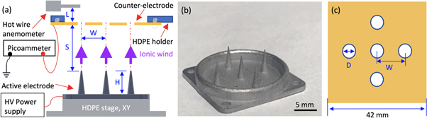
Figure 1. (a) Schematic of the experimental setup; (b) 5-needle active electrode binder inject-printed in stainless steel 316L; (c) schematic of copper plate counter-electrode. In the schematics, L is the separation between the inlet of the anemometer and the exit plane of the ionic wind pump, H is the height of the needles, W is the inter-needle separation, S is the separation between the tips of the active electrode and the counter-electrode, and D is the diameter of the counter-electrode apertures.
Download figure:
Standard image High-resolution image2.2. Active electrode fabrication
The active electrodes were monolithically fabricated in SS 316L via inkjet binder printing [31] (DM P2500, Digital Metal, Hollsopple, PA, USA) using a CAD file in STL format (SolidWorks, Dassault Systémes, Waltham, MA, USA); binder inkjet-printed SS 316L has been shown to resolve finer features than the other mainstream metal printing methods (minimum feature size ∼300 μm), is chemically resistant, has low porosity, and exhibits electrical resistance, thermal conductivity, and Young's modulus close to bulk values [32]. Two versions of the active electrode were printed, i.e. a five-needle version, and a single-needle version –the latter version was used to benchmark the performance of the multi-needle devices. The as-printed conical needles of the active electrode have a base radius equal to 863 μm ± 21.31 μm, a tip radius  equal to 151.3 μm ± 3.25 μm, and a height H equal to 5.10 mm ± 0.31 mm.
The sharpness of the needles of the active electrode is limited by the resolution capabilities of the printing method; however, having sharper needles is advantageous as it would reduce the onset bias voltage of the ionic wind pump. Consequently, an electropolishing process was developed to overcome the restrictions of the printing method without sacrificing feature uniformity. A mix of 9 mL 85 wt% phosphoric acid, 6 mL 98 wt% sulfuric acid, and 5 mL distilled water was used as electropolishing solution. To conduct the electrochemical polishing, the part to be polished and a 1 cm by 6 cm SS plate are immersed in the solution while connected to a DC bias voltage using a power supply (DP832A model, RIGOL USA, Beaverton, OR, USA) –the anode of the power supply is connected to the part to be polished, while the cathode of the power supply is connected to the SS plate, and the current is kept constant; the SS plate is covered with a glass slide to help uniformize the etch. The amount of etching is time-controlled. The dependence of the tip radius, tip shape, and surface quality was explored by varying the current and etching time. Figure 2 shows the metrology of an active electrode with 32 needles before and after experiencing an electropolishing process for 40 min while drawing 0.9 A; before sharpening, the average tip diameter is equal to 302.6 μm ± 2.9 μm; after sharpening, the average tip diameter is reduced to 153.4 μm ± 4.3 μm.

Figure 2. Tip diameter distribution of an active electrode with 32 needles before and after electropolishing.
Download figure:
Standard image High-resolution imageEmpirically, it was determined that electropolishing at higher currents causes pitting and poor control of the shape of the tip due to the rapid electrolysis, while electropolishing at lower currents significantly slows down the etch rate; a low-current/high-current two-step process was found to yield the best results (fresh acid bath is prepared for each step). For the single-needle active electrodes, the first electropolishing step takes 30 min and draws 0.8A, yielding needles with 184.8 μm ± 4.1 μm tip diameter; the second step lasts 15 min and draws 1A, resulting in needles with 116.1 μm ± 2.3 μm tip diameter. Similarly, for the five-needle active electrodes, the first electropolishing step lasts 30 min and draws 0.5A, resulting in needles with 165.5 μm ± 6.3 μm tip diameter; the second electropolishing step takes 15 min and uses 0.8A, resulting in needles with 83.4 μm ±2.8 μm tip diameter. Consequently, in both cases (single-needle, multi-needle), the tip variation of the finalized needles is kept constant from as-printed values. A typical needle after each polishing step is shown in figure 3.

Figure 3. A tip of a needle part of a five-needle active electrode after electropolishing. (a) The active electrode is polished for 30 min while drawing 0.5A, uniformly reducing almost in half the tip diameter from as-printed values. (b) The active electrode receives a second electropolishing step for 15 min while drawing 0.8A, uniformly reducing almost in half the tip diameter from first-polishing step values.
Download figure:
Standard image High-resolution image2.3. Device characterization
Experimental characterization of the devices was conducted in air at room temperature and at atmospheric pressure; single-needle ionic wind pumps with the same needle geometry were also tested to benchmark the performance of the multi-needle devices. A high voltage power supply (0–20 kV 1 mA, Gamma Voltage Research, Ormond Beach, FL, USA) was used to apply a negative bias voltage to the active electrode, while the counter-electrode was grounded through a picoammeter (Keithley 485, Tektronix, Beaverton, OR, USA), triggering a negative corona discharge; during operation, ionic wind flows from the needles towards and through the apertures of the counter-electrode; the flow velocity at the center of the exit was measured by a hot wire anemometer (model 430, TSI Incorporated, Shoreview, MN, USA); The distance L between the probe of the anemometer and the collector plate was set at 17.5 mm (figure 1), far enough from the exit of the pump so that the electric field is not significantly altered by the presence of the probe. The influence of tip multiplexing and tip sharpening on the ion current, airflow velocity, volumetric flow rate, and kinetic conversion efficiency of the ion wind pumps were characterized under different interelectrode separations (i.e. 4 mm, 5 mm, 5.35 mm, 6 mm, 7 mm, 7.85 mm, 9 mm, and 10.35 mm), counter-electrode aperture diameters (i.e. 3 mm and 5.5 mm), and applied bias voltages (continuously varied between 4 kV and 17 kV).
2.4. Scaling analysis
Based on conservation of momentum, in a single-needle ionic wind pump the local air velocity  of a negative discharge ionic wind pump is related to the density of the electrohydrodynamic force
  via
via

where  = 1.225 Kg m−3 is the density of air; the electric force density can be approximated as

where  is the number density of the negative ions,
  is the electric field, and r is the radial distance from the spherical tip surface (spherical coordinates). Peek's formula of the electric field between two parallel wires [33] was adapted to estimate the electric field distribution of the needle-plate geometry (having a tip facing a plate at a certain distance is equivalent to having two tips facing each other at twice the distance –the plate is the symmetry plane), given by

in which  is the applied bias voltage,
  is the interelectrode distance, and
  is a dimensionless parameter defined as

where  is the tip radius of the needle. Equation (3) was validated by comparing its predictions with those from COMSOL Multiphysics simulations of the same setup. The electric field is maximum at the tip of the electrode
  and is equal to
  In Poisson's equation, with only one species accounted (negative ions), the electric field is expressed in spherical coordinates as

where  is the charge of negative ions and
  is the electrical permittivity of air (i.e. 8.85 × 10⁻¹² C2 N−1 m−2). Integrating over the ionization region, which corresponds to the region near the tip where the electric potential increases from the onset potential
  (Kaptzov's assumption) to the actual potential
  applied on the tip, the total charge
  being transported from the tip is given by

where  is the radius of the ionization boundary, estimated from Kaptzov's assumption, which is of the same order of magnitude of
  The difference between the applied bias voltage and the onset voltage
  is known as the overvoltage. The electric field
  at
at  is calculated based on Kaptzov's assumption, i.e. the potential at the ionization boundary is maintained at
  (the corona onset voltage) during the corona process regardless of the potential applied at the tip. Thus, the averaged number density of the negative ions is calculated as

by integrating the momentum equation across the interelectrode separation, the velocity at the exit,  can be calculated as

The current I measured at the electrode can be expressed as
where  is the mobility of the negative ions and
  is the drift velocity of the negative ions propelled by the electric field
  Consequently,
  is
is

Therefore, for a given device with a fixed tip radius, the only relevant geometric parameter that influences the velocity of the flow is the interelectrode separation  Moreover, for a given wind velocity, the volumetric flow rate increases with the area of the counter-electrode apertures, which is directly related to the diameter aperture
  Consequently, the size of the exit apertures and interelectrode separation were varied in the experiments to optimize the flow velocity (see section 2.3). The wind velocity increases with smaller tip radius and larger onset voltage
  which decreases with larger tip radius; therefore, for a given tip size, the velocity of the flow can be optimized.
2.5. Device modelling
In this study, a two-module model that efficiently and effectively predicts the long-time airflow from the short-time corona discharge process was implemented in COMSOL Multiphysics (COMSOL, Inc., Burlington, MA, USA) for a single needle in a 2D axisymmetric geometry shown in figure 4. The needle is biased at a negative voltage and acts as the active electrode of the corona diode, near which ionization takes place. The plate counter-electrode is grounded, and its aperture is centred on the axis of the needle. The tip of the needle is spherical and has a radius of 150 μm, which is the nominal value of the as-printed needles used in the experiments; the side slope of the needle is the same of the printed devices, but the height of the needle without the spherical tip is 3 mm, truncated from the 5 mm value in the printed needles to save simulation time. The radius of the counter-electrode aperture is equal to 1.5 mm, which corresponds to one of the apertures explored in the experiments. The distance between the electrodes is set at 7.85 mm, which is one of the inter-electrode distances used in the experiments. The boundary conditions are chosen to resemble the experimental conditions. The voltage was ramped up with a hyperbolic tangent function with time constant equal to 1 × 10⁵ s. A non-uniform spatial mesh was used for an accurate and efficient numerical treatment of discharge phenomena: on the one hand, near the electrodes, where the electric field variation is particularly strong, a very spatially fine mesh is used to resolve the steep gradients associated; on the other hand, away from the axis of symmetry and electrodes, a spatially coarser mesh is used as the field does not greatly vary there.

Figure 4. Meshed simulation geometry of a single-needle, single-aperture device.
Download figure:
Standard image High-resolution imageThe first module of the model is a three-species fluid model that takes into account major corona processes (e.g. ionization, detachment, attachment, electron-ion recombination, and ion-ion recombination) in the inter-electrode space, as well as secondary electron generation on the surface of the active electrode; the second module is a gas dynamics model. With the EHD force distribution calculated from the corona model in a roughly time-independent region, the airflow characteristics can be predicted. This one-way coupling from the corona model to the gas flow model is possible because of the significant differences between the flow velocities, i.e. the low-speed airflow does not alter the transport of the charged species. Each of the charged species in the interelectrode space is described by a fluid model using the continuity equation

where  represents the three species in this model, i.e. electrons, positive ions, and negative ions;

 and
and  are the number density, flux, volumetric source and charge of each species, respectively; the flux is given by

The flux is related to the drift under the electric field by the velocity  with
with  the electric field,
  the mobility of charged species k, and
  the rate of the diffusion driven by the number density gradient of species k. In the simulations, the mobilities of the positive and negative charged molecules are
  m2 V−1 s−1 and
  m2 V−1 s−1, respectively, and the diffusivities were calculated as
  where
where 
 is Boltzmann's constant,
  is the species temperature, and
  is the species charge [34].
The continuity equation relates the rate of density change of each species to the drift and diffusion under the electric field, as well as the generation and consumption of species through major discharge processes (the volumetric source term  ), i.e. ionization, detachment, attachment, electron-ion recombination, and ion-ion recombination. This model is based on the single-moment approximation, which is valid for up to 1500 Td fields under atmospheric pressure [26]. The rate coefficient of each process is a function of the local electric field and the parameters are taken from literature [35, 36]. Specifically, the reduced ionization coefficient, reduced two-body attachment coefficient, electron energy, and reduced electron mobility (
 where
where  is the neutral number density
  ) as a function of the reduced electric field are plotted in figure 5.

Figure 5. Simulation parameters as a function of reduced electric field: (a) reduced ionization coefficient, (b) reduced two-body attachment coefficient, (c) electron energy, (d) reduced electron mobility.
Download figure:
Standard image High-resolution imageThe electric field is solved from Poisson's equation, taking into account space-charge effects


where  is the electrical permittivity of air and
  is the electric potential applied to the needle. The coupled set of equations (11)–(14) is self-consistent and describes the evolution of the corona discharge, providing information about the spatial and temporal behaviour of charged species and local electric fields. The EHD force that drives the flow is expressed as a function of the charge density and the electric field, i.e.

The flow can adequately be described as incompressible (the characteristic Mach number, i.e. 0.017, estimated with the maximum flow velocity measured in the experiments, i.e. ∼6 m s−1 {see sections 3.1 and 3.2}, is far smaller than the threshold for a fluid to show compressibility effects, i.e. 0.3 [37]); therefore

The open-boundary flow is treated as laminar flow; the flow is modelled as Newtonian, with constant density and viscosity. Therefore, the airflow is described by the Navier-Stokes equation with the EHD force equal to a body force

where  and
and  are the density and viscosity of dry air, respectively. The secondary electrons that sustain the discharge are accounted as the boundary condition of the active electrode

with n the surface normal and γ the secondary electron emission coefficient. In the simulations, γ is set at 0.001 (the value falls in the middle of the range of reported values, i.e. 10−6 – 10−1 [34, 36, 38, 39]; also, theoretical estimates based on the onset of the corona discharge using the Townsend breakdown criterion, the streamer breakdown criterion, or indirect electron production mechanism show good agreement with experimental data for values of γ between 10−4 and 10−3 [39]). Finally, the discharge current I is calculated by integrating the electron and ion flux in the simulation domain caused by drift and diffusion

in which  is the Laplacian field (i.e. the electric field when no space charge is present).
3. Results and discussion
3.1. Experimental characterization—as-printed tips
Typical current versus voltage characteristics of an as-printed single-needle device are shown in figure 6(a); the onset voltage  (estimated from the Townsend's relationship [40]) and the spark voltage
  (i.e. minimum bias voltage at which sparks are emitted) are reported in table 1. An ionic wind pump with
  = 3 mm and
  =4 mm features a narrow range of operational bias voltages, a sharp increase in current, and a fluctuating flow velocity. For as-printed devices operated at a high bias voltage, the corona discharge is unstable –this is particularly evident when the interelectrode separation is large, resulting in a pronounced rise of the current and a drop in the flow velocity. For values of interelectrode separation that result in stable operation, the data can be nicely grouped using the interelectrode distance, with negligible influence on the counter-electrode aperture diameter. As the interelectrode separation increases, the onset voltage, spark voltage, and operating voltage range (i.e. range of voltages between the onset voltage and the spark voltage) also increase. For devices with
  = 3 mm, the current has a negligible increase with interelectrode separation beyond
  = 9 mm. A larger aperture generally results in a slightly higher onset voltage and a lower spark voltage. Stable currents as high as ∼150 μA were measured.

Figure 6. Performance of as-printed single-needle ionic wind pumps versus bias voltage: (a) current; (b) flow velocity; (c) volumetric flow rate; (d) kinetic conversion efficiency. Solid markers denote stable operation, while hollow makers denote unstable operation.
Download figure:
Standard image High-resolution imageTable 1. Onset and spark voltages of the as-printed, single-needle devices for different interelectrode separations and counter-electrode apertures.
| S (mm) | 4 | 5 | 5.35 | 6 | 7 | 7.85 | 9 | 10.35 | ||||||||
|---|---|---|---|---|---|---|---|---|---|---|---|---|---|---|---|---|
| D (mm) | 3 | 5.5 | 3 | 5.5 | 3 | 5.5 | 3 | 5.5 | 3 | 5.5 | 3 | 5.5 | 3 | 5.5 | 3 | 5.5 |
 (kV) (kV) |
4.0 ± 0.6 | 4.7 ± 0.4 | 4.5 ± 0.3 | 5.0 ± 0.5 | 5.0 ± 0.4 | 5.3 ± 0.6 | 5.2 ± 0.2 | 5.3 ± 0.4 | 5.4 ± 0.5 | 5.8 ± 0.3 | 6.2 ± 0.5 | 6.1 ± 0.3 | 6.7 ± 0.6 | 7.1 ± 0.4 | 6.5 ± 0.5 | 7.8 ± 0.7 |
 (kV) (kV) |
6.6 ± 0.3 | 6.8 ± 0.5 | 8.2 ± 0.6 | 7.8 ± 0.8 | 9.4 ± 0.7 | 9.0 ± 0.4 | 9.8 ± 0.5 | 10.0 ± 0.7 | 11.4 ± 0.8 | 11.2 ± 0.6 | 13.6 ± 0.6 | 13.2 ± 0.8 | 15.2 ± 0.7 | 14.8 ± 0.7 | 14.8 ± 0.7 | 17.2 ± 0.9 |
The dependence of the flow velocity and volumetric flow rate on the bias voltage is shown in figures 6(b) and (c), respectively. The flow velocity is a function of the interelectrode distance  with smaller
  resulting in larger flow velocity at a given bias voltage –following the prediction of the scaling analysis presented in section 2.4, where the velocity is inversely related to the interelectrode separation. Moreover, a smaller interelectrode separation can reduce the onset voltage of the device, increasing the overvoltage –these synergetic effects make possible to design a miniaturized pump with high flow velocity. On the one hand, the maximum flow velocity increases with increasing interelectrode separation, which is caused by the associated larger spark voltage. On the other hand, with a smaller interelectrode distance, or while operating the device at a lower bias voltage, airflow from a larger counter-electrode aperture has a larger velocity –the difference gradually vanishes as the interelectrode separation or the applied bias voltage increases. A larger counter-electrode aperture generates a higher volumetric flow rate because the flow velocity increases with the size of the aperture. For all interelectrode distances tried in the experiments, the volumetric flow rate produced with the 3 mm aperture follows a straight line as shown in figure 6(c).
The pump efficiency  given by

is used to benchmark how much electrical energy is converted to kinetic energy. The estimates of the pump efficiency are shown in figure 6(d); the error bars of the pump efficiency data were calculated using Gauss' error propagation theory [41]. Large variation in the efficiency, especially right after the onset of corona discharge, is a result of the fluctuations in the current and velocity measurements, which are related to the nature of corona ionic wind and the equipment used to collect the experimental data. Fluctuations in the current and the flow velocity of corona ionic wind devices have also been observed by other authors [42]. The efficiency increases with the counter-electrode aperture diameter because a larger aperture produces a larger volumetric flow rate for a given power consumption level. On the one hand, the efficiency of the device with smaller aperture (D = 3 mm) is roughly constant for varying interelectrode separation, suggesting that in such configuration the device has associated an efficiency limit. On the other hand, the efficiency for the devices with D = 5.5 mm is optimal around 7 mm interelectrode separation.
Typical current, flow velocity, volumetric flow rate, and efficiency characteristics of as-printed five-needle ionic wind pumps are shown in figures 7(a)−(d), respectively. The scaling analysis described in section 2.4 is no longer applicable due to the interference between tips (electric field shadowing); in particular, the onset voltage of these devices is larger than that of the single-needle devices. The operating voltage range is narrower in these devices compared to the single-needle devices because of the fast accumulation of ions in the interelectrode space, inducing sparks at a smaller bias voltage compared to the single-needle devices. For a given bias voltage, the per-needle current in the five-needle devices is smaller than the current emitted by the single-tip devices; however, the slope of the total current-versus-voltage characteristics is steeper. At large interelectrode separation ( > 9 mm), the current-voltage characteristic of the five-needle devices is independent of the inter-electrode separation and the counter-electrode aperture size (figure 7(a)). The increase in maximum velocity for a device with larger interelectrode separation is not as noticeable as in the single-needle devices. Due to electric field shadowing, the flow velocity at the tip in the middle of the array is slightly lower than that from the peripheral apertures, and, overall, the velocity is lower than in the single-tip device case, which is above 5 m s−1. A larger aperture tends to boost the airflow (figure 7(b)), especially at higher overvoltage or larger interelectrode separation, generating significantly larger flow rates than the single-needle device case.

Figure 7. Performance of as-printed five-needle ionic wind pumps versus bias voltage: (a) current; (b) flow velocity; (c) volumetric flow rate; (d) efficiency. All markers are solid, denoting stable operation.
Download figure:
Standard image High-resolution imageFor the range of geometries and conditions tested in the experiments, the best-performing as-printed, multi-emitter ionic wind pump has  = 6 mm and
  = 5.5 mm, and is operated at
  = 7.4 kV. At this bias voltage, the pump consumes 0.5 W (i.e. 2.5 times the power consumption of the corresponding single-needle pump) and could generate flow with 2.66 m s−1 velocity (slightly lower than the single-tip device, i.e. 3 m s−1) and 316 cm3 s−1 volumetric flow rate (i.e. two times higher than the single-needle device) with 0.27% efficiency (35% higher than the single-tip device, which is 0.2%). The bias voltage associated with the optimal operation of the ionic wind pump falls right in the middle of the operating voltage range (i.e. 6.2 kV – 8.8 kV), which means that this pump is stable, without significant charge accumulation during operation (e.g. we did not encounter any sparks during one-hour-long experiments).
3.2. Experimental characterization–sharpened tips
The experimental characterization of the electrochemically polished single-needle ionic wind pumps is shown in figure 8; the onset voltage and the spark voltage of the devices are reported in table 2. Compared with the as-printed single-tip devices, the devices with sharper tips are stabilized at a smaller interelectrode distance (solid red triangles in figures 8(a) and (b)); however, at  = 2 mm, a sharpened device with 3 mm diameter aperture is not stable; similar sharp current increase can be observed at the pre-breakdown stage in devices with
  = 3 mm,
  ≤ 4 mm and with
  = 5.5 mm,
  ≤ 6 mm. Devices with sharpened tips have a lower spark overvoltage compared to the unpolished devices. Analogous to the devices with unpolished needles, a larger counter-electrode aperture results in larger flow velocity, and the increase in flow velocity diminishes for large interelectrode separation (
 = 8 mm and 9 mm, figure 8(b)). Biased at the same voltage, pumps with sharper needles propel air faster because of the significant decrease in the onset voltage (table 2, on average 18% less than that of the unpolished devices). However, no significant difference in the kinematic conversion efficiency of the pumps with unpolished and polished needles was observed given that the current consumed by the pumps with sharper tips also increases (figure 8(d)). The maximum velocity achieved by the pumps of the same exit size at a certain interelectrode separation is comparable, regardless of the diameter of the tips. Therefore, other methods to boost up the maximum velocity and the kinematic conversion efficiency in single-needle devices need to be explored.

Figure 8. Performance of electropolished single-needle ionic wind pumps versus bias voltage: (a) current; (b) flow velocity; (c) volumetric flow rate; (d) efficiency. Solid markers denote stable operation, while hollow makers denote unstable operation.
Download figure:
Standard image High-resolution imageTable 2. Onset and spark voltages of the electrochemically polished, single-needle devices for different interelectrode separations and counter-electrode apertures.
| S (mm) | 2 | 3 | 4 | 5 | 6 | 7 | 8 | 9 | ||||||||
|---|---|---|---|---|---|---|---|---|---|---|---|---|---|---|---|---|
| D (mm) | 3 | 5.5 | 3 | 5.5 | 3 | 5.5 | 3 | 5.5 | 3 | 5.5 | 3 | 5.5 | 3 | 5.5 | 3 | 5.5 |
 (kV) (kV) |
2.9 ± 0.1 | 2.9 ± 0.1 | 3.1 ± 0.2 | 3.1 ± 0.2 | 3.6 ± 0.1 | 3.6 ± 0.1 | 4.1 ± 0.2 | 4.1 ± 0.2 | 4.3 ± 0.4 | 4.4 ± 0.3 | 5.1 ± 0.3 | 5.4 ± 0.2 | 5.4 ± 0.3 | 5.7 ± 0.4 | 5.7 ± 0.4 | |
 (kV) (kV) |
5.4 ± 0.2 | 4.8 ± 0.2 | 5.8 ± 0.2 | 6.0 ± 0.3 | 6.8 ± 0.3 | 7.2 ± 0.4 | 8.4 ± 0.4 | 9 ± 0.4 | 9.4 ± 0.2 | 11 ± 0.5 | 10.8 ± 0.3 | 12.8 ± 0.5 | 11.4 ± 0.4 | 15.2 ± 0.5 | 13.2 ± 0.4 | |
The current-voltage characteristics at low bias voltage of sharpened five-needle devices with short interelectrode separation resemble those of the single-needle unpolished counterparts (figure 9(a)). For the five-needle devices with a 3 mm diameter aperture, a smaller interelectrode distance results in higher flow velocity at a given bias voltage–following the scaling analysis of a single-needle device. Although ionic wind pumps with sharper needles are capable of inducing higher velocity, as the interelectrode separation increases, the boost in flow velocity fades down.

Figure 9. Performance of electropolished five-needle ionic wind pumps versus bias voltage. (a) current; (b) flow velocity; (c) volumetric flow rate; (d) efficiency. All markers are solid, denoting stable operation.
Download figure:
Standard image High-resolution imageIn general, the efficiency of the polished five-needle devices is higher than the efficiency of the unpolished counterparts for all bias voltages (figure 9(d)). Compared with the as-printed devices, the electropolished five-needle devices turn on at a lower bias voltage and produce a higher velocity at a lower bias voltage. A polished five-needle pump with 5.5 mm apertures and interelectrode separation equal to 6 mm or 7 mm achieve both high flow velocity and high efficiency. For example, at 8 kV bias voltage, the as-printed, five-needle ionic wind pump with 7 mm interelectrode separation and 5.5 mm apertures generates a flow of speed 2.45 m s−1 with 0.23% efficiency while pumping 288 cm3 s−1 of air at standard conditions; with the same interelectrode separation and aperture diameter, operated at the same bias voltage (this is the bias voltage at which the single-needle pumps work optimally), the pumps with polished tips can generate a flow of 3.25 m s−1, i.e. 30.6% higher than the value from the unpolished, multi-tip device and has significantly higher efficiency (0.29%) and flow rate (379.6 cm3s−1).
The maximum velocity generated from the devices is roughly the same, regardless of whether the needles are polished, because the flow speed is mainly limited by the maximum bias voltage the device can sustain without producing sparks. Given that sharper tips greatly intensify the electric field and initiate breakdown at a smaller bias voltage, thereby devices with sharper tips do not excel in terms of boosting up the maximum velocity. Therefore, as with the single-needle devices, other methods to boost up the maximum velocity need to be explored.
3.3. Scaling analysis versus experimental data
The data from the polished and as-printed single-needle ionic wind pumps are in good agreement with the scaling analysis (section 2.4) as shown in table 3 –regardless of the size of the counter-electrode aperture. Furthermore, the current-voltage characteristics are largely independent of the diameter of the aperture for most of the parameters tested in the paper (S ≥ 5mm as-printed, S ≥ 2mm polished) when operating stably (see figures 6(a)−9(a)), supporting the use of equation (3) for the range of geometric parameters investigated in this study. In terms of the current (figure 10(a)), the linear fittings of  versus
  closely follow the experimental values (R2 ∼ 96%) and the slopes are within a factor of two of the theoretical value from the scaling analysis, i.e.
  = 1.50 × 10⁻¹⁴ A m V-2. In terms of the flow velocity (figure 10(b)), the linear fittings of
  versus
  reasonably follow the experimental values (R2 ∼ 70%) and the slopes are within 30% of the theoretical value calculated from the scaling analysis, i.e.
  = 2.69 × 10⁻⁶ m2 V−1 s−1. A slight deviation from the scaling analysis can be seen for devices with larger diameter apertures, which is related to the discrepancy in the electric field between a tip-plate geometry and the actual device with an aperture implemented. To compensate for the moderate dependence of the current on the size of the aperture, a dimensionless correction factor equal to
  is used, which makes the slopes of the linear fittings of
  versus
  very similar for all counter-electrode apertures, and close to the value calculated from our scaling analysis. Likewise, to compensate for the moderate dependence of the flow velocity on the size of the aperture, a second dimensionless factor is used; however, given that the ionic wind velocity is directly related to the current, which, as explained before, is to first order independent of the aperture of the counter-electrode, the influence on the velocity from the current and the aperture are relatively independent from each other. Consequently, the second correction factor is equal to the current scaling correction factor,
  times
times  which makes the slopes of the linear fittings of
  versus
  very similar to the value calculated from scaling analysis.
Table 3.
Slope of least-squares fitting curves  versus
  and
and  versus
  calculated from experimental data with and without correction factor (EW and EWO, respectively), and compared with theoretical estimates from scaling analysis.
| Parameters | Slope of  versus versus  
|
Slope of  versus versus  
|
|||
|---|---|---|---|---|---|
| As printed | Polished | As printed | Polished | ||
| D = 3 mm | EWO | 8.27 × 10⁻¹⁵ | 7.64 × 10⁻¹⁵ | 4.10 × 10⁻⁶ | 3.58 × 10⁻⁶ |
| EW | 1.16 × 10⁻¹⁴ | 1.08 × 10⁻¹⁴ | 3.13 × 10⁻⁶ | 3.02 × 10⁻⁶ | |
| Scaling | 1.50 × 10⁻¹⁴ | 2.69 × 10⁻⁶ | |||
| D = 5.5 mm | EWO | 7.62 × 10⁻¹⁵ | 1.03 × 10⁻¹⁴ | 3.61 × 10⁻⁶ | 3.49 × 10⁻⁶ |
| EW | 9.32 × 10⁻¹⁵ | 1.21 × 10⁻¹⁴ | 2.41 × 10⁻⁶ | 2.89 × 10⁻⁶ | |
| Scaling | 1.50 × 10⁻¹⁴ | 2.69 × 10⁻⁶ | |||

Figure 10. Scaling anaysis of data from single-needle ionic wind pumps. (a) Curve fitting of  versus
  (b) Curve fitting of velocity ploted as
  versus
  In the plots, solid markers denote as-printed devices, while hollow markers denote electropolished devices.
Download figure:
Standard image High-resolution imageThe scaling analysis and correction factors reported in this work provide valuable insights on the physics of the operation of the corona pump, e.g. the dependence of the velocity on the current and the counter-electrode aperture, which can be used as a guidance to tune the design of the pump for optimal performance. Although the deviation of the scaling analysis can be compensated by adding correction factors, it is not generic —an improved understanding of how the aperture size and other parameters in the setup influence the behaviour of the pump is necessary to gain better insight of the physics and to guide the design of a more efficient and effective compact ionic wind pumps. Furthermore, the experimental behaviour of the five-needle devices is different from the single-tip devices and does not follow the scaling analysis in general. Understanding of the interference between tips might be crucial to design more efficient and effective multi-needle devices.
3.4. Generation of Trichel pulses
The simulations of the DC corona focused on studying ultra-short Trichel pulses, which has an associated period that is the natural timescale of the dynamics of the corona discharge; based on this characteristic time, we can infer the airflow since the behavior of the EHD force that drives the flow is directly related to the dynamics of the charged species. The simulations were run on a workstation Lenovo ThinkStation P920 (Lenovo, Morrisville, NC, USA) with two CPUs Intel Xeon Gold 5118 (each CPU with 12 cores, 24 threads, and 16.8 MB cache), 3.2 GHz of clock, 96 GB of RAM memory and 4TB of solid-state hard disks; it took around 10 days to simulate 2 ms for a given set of parameters, an numerous simulations were made while varying the geometric parameters of the pump to conduct the study. The Trichel pulses shown in figure 11 were calculated with an applied bias voltage equal to −6 kV. Each pulse has a peak current of around 1.5 mA, and the peaks have a repetition frequency of 153 kHz; these values are comparable with data published by other authors [34]. The rise time of each pulse is around 25 ns, while the pulse falls in approximately 65 ns. The number density of each species and electric field are shown in figure 12, sampled at the times marked in figure 11(b). At the beginning of the pulse, the electron and ion number densities start to increase due to ionization near the active electrode because the electric field is higher than the threshold. Due to the short distance to the active electrode and the relatively high drift velocity, positive ions are soon attracted to the active electrode, resulting in a decrease of the electric field in its proximity and in a narrower ionization region. The number density of the negative ions starts to increase as electrons are pushed away from the active electrode, and get attached to neutral gas molecules –mainly oxygen. At the peak current, an overall positive space charge occupies the volume near the needle (region within ∼40 μm from the surface of the tip), while a slightly negative space charge fills-in the rest of the interelectrode space with a peak at 80 μm from the tip surface; the negative net charge in the interelectrode space decreases the electric field and quenches the avalanche ionization. Only after the negative cloud travels enough distance away from the tip (750 μm in the simulated setup), the electric field distribution returns to the state that is not heavily distorted by the presence of the ions, and its value near the tip goes back to the ionization threshold. Given that the distance the negative cloud travels is much larger than the length of the ionization region, although the drifting speed of negative ions is slightly larger than that of the positive ions, the decaying tail is much longer than the rise time and the time interval calculated from the traveling time of negative ions corresponds well with the time interval of the Trichel pulses. The number density of the positive ions peaks at 60 μm from the tip surface when the pulse forms; when ionization intensifies, the peak is pulled slightly towards the active electrode. For negative ions and electrons, the maximum densities move further away from the needle tip, at around 180 μm, and move to 28 μm from the needle tip at the peak. At the peak, the magnitude of the electric field near the tip drops dramatically (shown in the inset of electric field distribution plot figure 12(d)) because the positive ions are the dominant species and are confined within the region near the tip. The edge of this valley is at the point where the polarity of the net number density of charged species switches from positive to negative, and is associated with the negative ion generation.

Figure 11. (a) Trichel pulse sequence; (b) close-up of Trichel pulse peaked at 87.655 μs from (a).
Download figure:
Standard image High-resolution image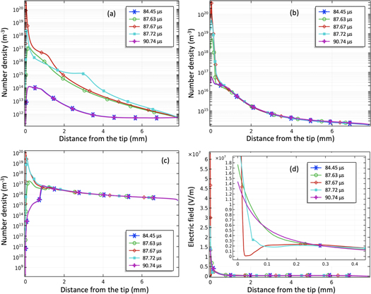
Figure 12. Number density for (a) electrons, (b) positive ions, and (c) negative ions, and (d) electric field distribution along the symmetric axis with inset of the 0–0.4 mm region of a needle during a Trichel pulse.
Download figure:
Standard image High-resolution image3.5. Estimation and characterization of EHD forces
The EHD forces that drive the airflow are directly related to the distribution of the electric field and the number density of the charged species; therefore, the periodic behaviour of the EHD forces and the Trichel pulses are similar. The EHD force in the z-direction (see figure 4) is shown in figure 13, which is calculated from the results of the corona model sampled from one pulse period at time (a) 87.629 μs, (b) 87.655 μs, (c) 87.72 μs, and (d) 90.74 μs –the same times sampled in figure 11(b). Before the pulse formation, positively charged species dominate in the interelectrode space and the EHD force in the z-direction points downwards, driving the flow towards the negatively biased tip. During the pulse, there are two distinct regions for the force: one region, near the tip, is characterized by a negative force, while the second region, i.e. the majority of the interelectrode space, provides a positive force that drives the gas molecules forward, towards the counter-electrode; this positive force is three orders of magnitude smaller than the negative force. The force in both the positive and negative regions first increases on the rising edge of a current pulse, to then decrease at the pulse tail. The negative force region is compressed as the Trichel pulse forms because the positive charges are confined near the cathode during ionization. Negative ions are the dominant species in the drift region, which contributes to the positive force that drives the flow towards the collector.

Figure 13. Force per unit of volume in the z-direction, sampled from one pulse period at time (a) t = 87.619 μs, (b) t = 87.655 μs, (c) t = 87.72 μs, and (d) t = 90.74 μs.
Download figure:
Standard image High-resolution imageIn the radial direction (figure 14), a positive force region starts to build as the pulse is initiated; this is related to the extreme distortion of the electric field that changes its direction due to the overall positive net charge generated during ionization. The peak of this positive region moves away from the symmetric axis in the rising edge of the pulse, and gradually returns to the centreline during the pulse decay, along with the movement of the peak of the charged particles cloud. At the peak, the maximum radial forces shift to 35 μm away from the axis, corresponding to the shift of the peak net charge density, which is related to the huge number of positive ions generated in this region. At the current peak, the forces in r-direction in both negative and positive regions are of the same order of magnitude, and their maximum values drop simultaneously as the current decays and the region occupied with positive ions diffuses.

Figure 14. Force per unit of volume in the r-direction, sampled from one pulse period at time (a) t = 87.619 μs, (b) t = 87.655 μs, (c) t = 87.72 μs, and (d) t = 90.74 μs.
Download figure:
Standard image High-resolution image3.6. Averaged EHD force
As previously mentioned, the flow velocity of the charged species is two orders of magnitude higher than the airflow driven by the EHD forces. The Trichel pulse of the corona discharge is characterized by a timescale in the range of 100 nanoseconds and a repetition period on the order of 10 microseconds, which is not sufficient to form a hydrodynamically stable airflow. To simulate the airflow with reasonable precision, a considerably longer simulation time is required compared to the simulation time required to conduct the Trichel pulse calculation. To significantly reduce the computational cost of this task, while maintaining acceptable precision, a force in the short-timescale that is representative of the long-term behaviour needs to be chosen. The key insight is that the forces in r- and z-directions averaged over the whole simulation region are roughly constant over time.
The time-dependent forces in the r- and z-directions averaged over the simulation domain are shown in figure 15(a). The averaged force in the z-direction stabilizes after 150 μs, while the force in the r-direction reaches a relative constant after 250 μs. Moreover, the forces have the same periodic behaviour as the Trichel pulses, as shown in the inset of figure 15(a); therefore, a time averaging of the forces should entail a time interval that is a multiple of the Trichel pulse time. Consequently, taking into account the periodicity of the force, the forces employed for the flow calculation are averaged over two periods, i.e. from 300.19 μs to 306.90 μs, and shown in figures 15(b) and (c).

Figure 15. (a) Time evolution of the EHD force averaged over the simulation domain; (b) EHD force in the r-direction averaged over 300.19 μs to 306.90 μs; (c) EHD force in the z-direction averaged over 300.19 μs to 306.90 μs.
Download figure:
Standard image High-resolution imageFor a direct comparison between the experimental and simulated velocities from single-needle devices, the simulation region for flow calculation is extended to a larger domain that covers the downwind region where the anemometer is situated. The EHD force distribution in the r- and z-directions shown in figures 15(b) and (c) are calculated from the corona model implemented in COMSOL with a bias voltage equal to −6 kV and a counter-electrode diameter aperture equal to 3 mm. For these conditions, the airflow driven by the EHD force at other voltages are calculated by rescaling the forces with the aforementioned relationship  from the scaling analysis shown in section 2.4. Moreover, for devices with a different counter-electrode aperture (
 = 5.5 mm), the EHD forces are scaled by the relationship with the correcting term from the scaling analysis, i.e.
  which considers the influence of the size of the diameter aperture. Based on this method, the velocity of the single-needle devices at different bias voltages and counter-electrode apertures, measured experimentally and predicted from the EHD force calculated from the corona model is shown in figure 16 versus applied bias voltage. The predicted velocity agrees well with the experiments at low applied bias voltages; as the applied bias voltage increases, the predicted values are lower than the experiments, which might be related to the extreme amount of ion generation that failed to be captured by the scaling analysis. Another possible cause of the discrepancy is the fluctuations in the velocity measurements. Nonetheless, the results suggest that by combining scaling analysis and corona process simulation could largely reduce the simulation time and provide an adequate prediction of the airflow velocity.

Figure 16. Velocity at 17.5 mm downstream from the counter-electrode as a function of the applied bias voltage from estimates (diamonds) and experiments (squares) for a single-needle device. The figure includes one estimated data point from a COMSOL simulation (6 kV, 3 mm aperture), and the rest of the estimated data points come from applying the scaling analysis to the results of such COMSOL simulation.
Download figure:
Standard image High-resolution image
4. Conclusion
In this study, we reported the proof-of-concept demonstration of the first additively manufactured, miniature, metal multi-needle ionic wind gas pumps in the literature. The pumps are needle-ring corona diodes composed of a monolithically inkjet binder-printed active electrode, made in stainless steel 316L, with five sharp, conical needles, and a thin plate counter-electrode, made in copper, with electrochemically etched apertures aligned to the needle array; by applying a large bias voltage across the diode, electrohydrodynamically driven airflow is produced. The influence of tip multiplexing and tip sharpening on the ion current, airflow velocity, volumetric flow rate, and kinetic conversion efficiency of the pumps was characterized under different interelectrode separations, counter-electrode aperture diameters, and applied bias voltages, while triggering a negative corona discharge; the performance of the single-needle devices was also collected and used as benchmark. At the optimal operating bias voltage (7.4 kV), the as-printed five-needle ionic wind pump ejects gas at 2.66 m s−1 and at a volumetric flow rate of 316 cm3 s−1 –a twofold larger than the flow rate of a single-needle device with comparable efficiency (0.27%). With a two-step electropolishing procedure, the needles of the devices can be uniformly sharpened down to 83.4 μm ± 2.8 μm from 302.6 μm ± 2.9 μm as-printed values –i.e. over a threefold reduction in the tip diameter without increasing the absolute value of the diameter spread. Operated under the same conditions, the sharpened five-needle pumps can pump air with the same efficiency, but with 22% higher velocity (3.25 m s−1) compared to the unpolished devices.
A two-module model that considers the creation and consumption of the charged particles in the corona discharge process is proposed to simulate the ionic wind produced by the devices. The model, built in COMSOL Multiphysics, consists of a three-species corona module that is one-way coupled to the gas dynamics module. By rescaling the EHD body force, calculated from the corona model using a counter-electrode with 3 mm diameter apertures biased at −6 kV, the airflow velocity of single-needle devices with different aperture size and stressed at different bias voltages can be predicted; the results agree well with the experiments, especially when the applied voltages are not close to the breakdown voltage. Our results demonstrate that this method to estimate the long-timescale forces and flow can greatly reduce the simulation time given that the time-consuming EHD force calculation with the corona model can be avoided. Tentative directions for future research include (i) improving the reduced-order modeling to address the deviations between the predicted velocity from the scaling analysis and the experimental data at high bias voltages, (ii) studying the influence of the inter-needle electric field shadowing on the performance of the ionic wind pumps, and (iii) further exploring the design space to improve the performance the devices.
Acknowledgments
This work was sponsored in part by the Skolkovo Institute of Science and Technology–Massachusetts Institute of Technology Joint Next Generation Program.