


Abstract
I derive a figure of merit (FOM)  to estimate the maximum efficiency attainable by a generic non-ideal photovoltaic (PV) absorber in a planar single-junction solar cell. This efficiency limit complements the more idealized limits derived from fundamental physics, such as the Shockley–Queisser (SQ) limit and its subsequent generalizations. Specifically, the present FOM approach yields stricter efficiency limits applicable to realistic PV absorbers with various imperfections, including finite carrier mobilities and doping densities.
  is a function of eight properties of the absorber that are both measurable by experiment and computable by electronic structure methods. They are: band gap, non-radiative carrier lifetime, carrier mobility, doping density, static dielectric constant, effective mass, and two parameters describing the spectral average and dispersion of the light absorption coefficient.
  has high predictive power (absolute efficiency error less than
  ) and wide applicability range. The SQ limit and its generalizations are reproduced by
  . Simpler FOMs proposed by others are also included as special cases of
  .
.
Export citation and abstract BibTeX RIS

Original content from this work may be used under the terms of the Creative Commons Attribution 4.0 license. Any further distribution of this work must maintain attribution to the author(s) and the title of the work, journal citation and DOI.
1. Introduction
The goal of this paper is to develop a figure of merit (FOM) to assess the quality of a generic photovoltaic (PV) absorber. This FOM should establish a direct relationship between the key properties of the absorber material and the maximum efficiency achievable by the material when incorporated in a planar single-junction solar cell configuration under AM1.5G, 1-Sun illumination.
The efficiency η of such a solar cell depends on the properties of: (i) the absorber; (ii) the other constituent materials of the cell (e.g. passivation, [1] transport, [2] and contact [3] layers); (iii) the interfaces [4] between such materials; and (iv) the device architecture, i.e. the particular stacking and thicknesses of these materials. Directly measuring η requires fabrication of a complete solar cell, which is much more time-consuming than synthesis of the absorber alone. Besides this practical inconvenience, the quality of a PV absorber in a complete cell is often obscured by the concurrent effects of (i–iv) on the measured η. Hence, a method to predict the maximum efficiency  achievable by a PV absorber synthesized in the lab or modeled from first principles—and decouple this efficiency from effects (ii–iv)—would be desirable.
Some methods to achieve this goal already exist [5–11] but they have limitations. Even the most versatile efficiency prediction methods based on the principle of detailed balance [6–9] work under the assumption of perfect carrier collection efficiency, i.e. infinite carrier mobilities. When mobilities are finite (figure 1), these methods can still accurately predict open-circuit voltage ( ) limits, but may overestimate short-circuit currents (
 , figure 1(b)) and fill factors (FFs). Overall, these methods provide an upper bound to the real efficiency limit
  of a PV absorber. Inclusion of finite mobility effects in detailed balance methods has been proposed [12] but only in the radiative limit (i.e. infinite non-radiative carrier lifetime), with an energy-independent absorption coefficient, and no depletion region effects. Away from the radiative limit,
  could only be determined by explicit drift-diffusion simulation on a case-by-case basis [12, 13]. Thus, a general relationship between properties and maximum efficiency could not be established when including finite mobilities.

Figure 1. Dependence of the drift-diffusion-simulated efficiency η (a) and short circuit current  (b) on the thickness d of the PV absorber. Data is shown for an absorber with a 1.2 eV band gap at different lifetimes τ and mobilities µ. (a) When both τ and µ are sufficiently high, η approaches the SQ limit of 33.4% in the high thickness limit. If τ is high but µ is low, the PV absorber may still approach the SQ limit within a finite thickness range. The η versus d curves are roughly independent of µ at low thicknesses, but they drop more abruptly at high thicknesses when µ is low, due to imperfect carrier collection. The green lines indicate the optimal thickness
  for each value of τ (solid line for the high-µ case, dashed line for the low-µ case). The corresponding efficiency value is labeled
  and is assumed equal to the maximum efficiency
  attainable by the absorber. Note that d is a discrete variable in the simulations because each value of d requires a distinct simulation run. The simulated values of d are indicated by markers. (b) When µ is sufficiently high, the short circuit current is τ-independent over a wide thickness range, and it increases with thickness up to the SQ limit of 40
  . When µ is low,
  drops above a thickness threshold that increases with τ. This is due to the dependency of the diffusion and drift lengths on the µτ product.
Download figure:
Standard image High-resolution imageEfficiency prediction methods based on FOMs are rare for PV absorbers, even though FOMs are routinely employed to benchmark other types of energy materials, such as thermoelectrics [14] and transparent conductors [15, 16]. Some previously proposed PV FOMs [10, 11] consist of simple combinations of the light absorption coefficient α, the non-radiative carrier lifetime τ, and the carrier mobility µ. The ατ and  FOMs proposed by Kaienburg et al [10] seem to be the only FOMs with an explicit physical justification, so I will often refer to them in this article. Kaienburg et al found a logarithmic dependence of PV efficiency on the ατ FOM above a certain mobility threshold, and on the
  FOM below the threshold. This shift in FOM reflects the transition between perfect carrier collection (where changes in µ are irrelevant and the ατ FOM applies) to imperfect carrier collection (where changes in µ influence the efficiency and the
  FOM applies) [17].
While these FOMs are useful and intuitive, it is unclear if they can be generalized beyond the conditions studied by Kaienburg et al who kept all the absorber's properties fixed except for α, τ, and µ. In particular, the doping density was fixed to a low value to simulate a fully depleted absorber, and all the tested absorption coefficients had the same spectral shape. Different values of α were simply obtained by scaling the same spectrum by a constant value, and the maximum scaling factor was only 1.5 [10]. Other bulk properties that influence the efficiency, such as the static dielectric constant and effective density of states (DOS), were kept constant. Finally, an efficiency limit cannot be derived from the Kaienburg FOMs, because a unique quantitative relationship between these FOMs and PV efficiency was not established.
In this paper, I will propose an alternative phenomenological FOM, named  . To encompass a wide range of realistic PV absorbers, the
  FOM will be expressed as a function of additional relevant properties beyond α, τ, and µ. A PV efficiency limit
  will be uniquely defined as a function of
  and of the Shockley–Queisser (SQ) [5] limiting efficiency
  (figure 2). We will see that
  is a good estimator of
  , and that the Kaienburg FOMs are special cases of the more general
  FOM. As long as the relevant properties of the absorber are known, the
  limit can immediately be calculated from a single explicit equation, without having to first determine the optimal thickness by multiple calculations.
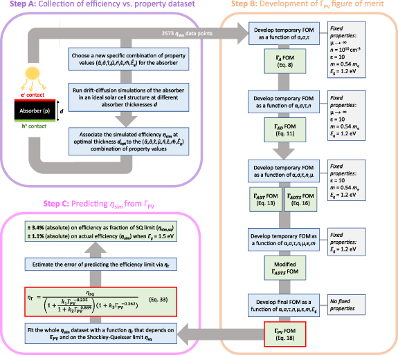
Figure 2. Workflow employed to predict the maximum efficiency  attainable by a realistic PV absorber described by eight bulk material properties (the
  set).
set).  is first estimated by the drift-diffusion-simulated efficiency
  for 2573 distinct combinations of properties (step A). Then an expression for a figure of merit is devised, with the goal of aligning the
  data points along a common curve, when plotted against the FOM. This is a stepwise development process, in which some properties are allowed to vary and others are kept fixed, a temporary FOM is devised, then new properties are allowed to vary and a new, more comprehensive FOM is devised (step B). This step culminates with the expression of the
  FOM, which is a function of all eight properties. In a last step, the
  versus
  data is fitted with a single function of
  , allowing us to estimate
  of any PV absorber with reasonable properties from its FOM (step C). The most important results of this study are outlined in red.
Download figure:
Standard image High-resolution image2. Methods
2.1. Definition of properties
An FOM for PV absorbers should be a function of the bulk material properties that have a significant influence on the realizable PV efficiency. I propose eight such properties: band gap  , non-radiative lifetime τ, carrier mobility µ, doping density n, static dielectric constant ε, DOS effective mass m, and two quantities (
 and σ) related to the spectral average and spectral dispersion of the absorption coefficient spectrum
  , respectively (λ is the wavelength of light). These eight bulk properties are the free parameters of the FOM (figure 2). I define the set of the eight properties as
  . Hence,
  . Defining these quantities is not trivial, so in the next paragraphs I will clarify the definitions used throughout this article.
 is defined as the weighted integral average of
  in the spectral region from
  nm to
nm to  , where h is Planck's constant and c is the speed of light.
  is the wavelength corresponding to the band gap energy.
  is a cut-off wavelength, chosen to disregard the very short wavelengths with negligible photon flux in the AM 1.5G spectrum, and for which
  data is often unavailable. The weights are given by the spectral density
  of the AM 1.5G photon flux. Thus:
The dispersion parameter σ is the weighted standard deviation of the logarithm of  in the same spectral region.
For a lighter notation, I will refer to the average absorption coefficient  simply as α in the rest of the article.
n is defined as the equilibrium concentration of electrons in the conduction band of the PV absorber in the dark without an applied voltage. When n is used as a parameter in a FOM, it is simply intended as the concentration of majority carriers regardless of their type (electrons or holes). Assuming homogeneous concentrations of fully ionized single acceptors and single donors ( and
and  , respectively):

This definition can easily be extended to the case of multiple types of fractionally ionized dopants that can donate/accept more than one electron.
The carrier lifetime τ is intended as the lifetime associated with non-radiative, Shockley–Read–Hall (SRH) recombination in the bulk [18, 19]. It is defined as:

Here,  is the thermal velocity of carriers in the material,
  is the concentration of the defects responsible for SRH recombination, and Σ is their carrier capture cross section. In general, electrons and holes may have different lifetimes
  and
and  , due to differences in their thermal velocities and (especially) capture cross sections by the dominant defect. To limit the number of free parameters in the FOM expression, I assume that
  . For a real PV absorber with significant differences between
  and
and  , it may still be possible to reduce the two separate lifetimes into an effective lifetime that can be used in the FOM, depending on the carrier injection level under illumination. This topic is discussed in the supplementary material. SRH recombination is assumed to be the only active recombination mechanism besides radiative recombination (Auger recombination is neglected).
The carrier mobility µ is defined from the conductivity effective mass M and the mean intra-band carrier scattering, or relaxation, time  as:
as:

where q is the elementary charge. Drift- and diffusion mobilities are assumed to be equal to each other. Analogous to the case of the SRH lifetime, different mobilities can generally be expected for electrons ( ) and holes (
 ) due to different values of M and
  in the valence- and conduction bands. Again, I assume
  to limit the number of free parameters in the FOM expression, but it may be possible to reduce carrier-specific mobilities into a single effective µ. A qualitative discussion is given in the supplementary material.
m is the DOS effective mass [20–23]. The DOS effective mass for electrons in the conduction band ( ) can be determined by considering the absorber's calculated electronic DOS, and fitting it with the following function near the energy of the conduction band minimum (
 ) [24]

where  (h is Planck's constant). An analogous expression is used to determine the DOS hole effective mass
  near the energy of the valence band maximum
  . Similar to the cases of τ and µ, electrons and holes generally have separate values for their DOS effective masses (
 and
and  , respectively). To avoid an exceedingly large number of free parameters in the FOM, I assume
  throughout this paper. However, it is straightforward to reduce
  and
and  to a single effective value
  without a significant loss of generality, as explained in the supplementary material. Note that m and M are not equivalent, since they are derived differently and have different physical meanings [21, 22].
The static dielectric constant ε is intended as the value of the dielectric constant in the limit of zero frequency (indicatively, below  ). Because both ions and electrons can respond to these low-frequency electric fields, ε is a measure of the polarizability of the PV absorber by both ionic and electronic displacements.
The band gap  is intended as the electronic band gap in the bulk of the absorber:

where  and
and  are the edges of extended bulk electronic states making up the conduction- and valence band, respectively. The SQ limit in this article is always calculated from this definition of
  . The electronic gap defined in equation (7) is always assumed to be equal to the optical band gap, i.e. the photon energy of absorption onset. This equality is enforced by only considering expressions for
  in which
  when
when  , and
, and  when
when  (E is the photon energy). Sub band gap absorption due to, e.g. excitonic absorption, defect absorption, or potential fluctuations is not considered. In the presence of sub band gap absorption,
  in its present definition may be difficult to measure and may not represent the most PV-relevant band gap value [25, 26]. In such cases, the PV-relevant band gap definition proposed in [26] may be more appropriate.
Throughout this paper, I assume all properties to be isotropic for simplicity. The implications of direction-dependent properties [27] are briefly discussed in the supplementary material.
As we will see, the definition of the  FOM includes polynomial functions with fractional exponents, as well as transcendental functions (exponential and logarithmic). To avoid complications and inconsistencies with units, it is necessary to convert the eight properties in the
  set to a unitless form [28] when they are used in an FOM. Throughout this article, the unitless versions of the eight properties are
  ,
,  ,
,  ,
,  ,
,  , and
, and  . m0 is the rest mass of the electron. σ and ε are already unitless.
2.2. Collection of reference efficiency-versus-property dataset
Once defined, an FOM for PV absorbers should enable a quantitative estimate ( ) of the maximum efficiency
  achievable by a candidate PV absorber with any (realistic) specific set of properties
  . Before attempting the definition of an FOM, it is therefore necessary to collect a dataset of
  versus
  to be used as a benchmark when evaluating the quality of a proposed FOM. This is step A in the overall workflow of this paper, shown in figure 2.
A reliable source for  for an absorber with a property set
  is a finite-element-based, one-dimensional drift-diffusion simulation of an ideal solar cell incorporating such an absorber. In this work, I have conducted these simulations with the SCAPS program [29]. In the ideal solar cell there are no efficiency losses due to contact layers, interfaces, or a non-optimal device structure. Instead, all efficiency losses with respect to the SQ limit
  can be attributed to non-optimal values in some of the bulk properties in the
  set. In practice, the simulated solar cell structure simply consists of the PV absorber and two contacts that are fully carrier-selective. Relying on one-dimensional simulations automatically implies another ideal feature, i.e. that the absorber's properties are homogeneous in the plane of the solar cell, which is often not the case in real materials [30]. All simulation parameters used to model this ideal device structure are shown in table S1, supplementary material.
The requirement for an optimal device structure implies that the drift-diffusion simulation used to estimate  must be carried out at the optimal thickness
  , i.e. the absorber thickness at which the highest efficiency is reached [10]. The computational procedure to obtain
  is visualized in figure 1(a). Briefly, a batch of simulations is executed at different absorber thicknesses d for each unique set of material properties
  considered in this work. The thickness at which η is maximized is taken as the optimal thickness
  for that particular
  property set, and the corresponding value of η is defined as
  for that particular
  property set (figure 1(a)). The consistency of the drift-diffusion-simulated values of
  ,
,  , FF, and
  with their maximum values allowed by the SQ limit is shown in figure S1, supplementary material.
I assume that  is a good estimator of
  (
( ) due to the ideality of the simulated solar cell structure. Thus, a dataset of
  values for various combinations of properties can be used as a training set to assess the appropriateness of various possible expressions of
  , in a similar spirit to machine learning approaches. When collecting the training dataset, it is important to sample different combinations of the eight properties within physical ranges. The property ranges sampled in this work are shown in table 1. In total, I employ a dataset of 2573
  values to derive the
  FOM. The device simulation workflow used to collect these values is summarized in step A of figure 2. All eight properties are changed independently of each other. For example, µ is not automatically changed when changing m, even though µ is likely to depend on m, everything else being equal. Likewise, α and σ are not automatically modified when changing
  , even though the actual
  spectrum is adjusted to ensure that the energy at which
  becomes greater than zero always corresponds to
  (see also previous section). Additional assumptions, approximation, definitions, and neglected physical phenomena are given in the supplementary material.
Table 1. The eight bulk properties of the absorber ( set) entering the definition of the
  FOM. The 'Sampled range' column gives the minimum and the maximum value of each property in the
  versus
  dataset. Since the
  FOM has been developed from data within these ranges, the efficiency prediction (
 ) for a PV absorber with properties falling outside of the sampled range may be grossly incorrect. The 'Default value' column gives the value used for each property when that property is kept fixed. In some figures in this article, data is shown for 'high' and 'low' values of a certain property. The 'high' and 'low' values are also given in the same column. Unitless versions of these properties (i.e. the property divided by its unit) are used in all figures of merit in this article.
| Property | Symbol | Unit | Sampled range | Default value |
|---|---|---|---|---|
| Band gap |

| eV | (0.7, 2.0) | 1.2 |
| Average of absorption coefficient | α |

|
|
 ('high': ('high':  ; 'low': ; 'low':  ) ) |
| Dispersion of absorption coefficient | σ | (0.2, 1.8) | 0.33 (with 'high α': 0.33; with 'low α': 1.42) | |
| SRH recombination lifetime | τ |

|
| Never fixed |
| Carrier mobility | µ |

|
|
 ('high': ('high':  ; 'low': 1) ; 'low': 1) |
| Doping density | n |

|
|
 ('high': ('high':  ; 'low': ; 'low':  ) ) |
| Static dielectric constant | ε | (1, 100) | 10 ('high': 100; 'low': 1) | |
| DOS effective mass | m | m0 | (0.12, 2.5) | 0.54 ('high': 2.5; 'low': 0.12) |
Throughout this paper, PV efficiencies will be expressed either as absolute power conversion efficiencies ( and
and  ), or as fraction of the maximum efficiency
  allowed by the SQ limit [5, 31] for an absorber of band gap
  . Such SQ-normalized efficiencies are labeled
  and
and  .
.
3. Results
The goal of the  FOM is to give an estimate
  of the efficiency limit of a real PV absorber. This estimate should be as close as possible to the corresponding
  benchmark obtained by explicit drift-diffusion simulation. Two logical steps are required to ensure good efficiency estimates across a wide range of potential PV absorbers that may have very different properties. First, we must define
  from the eight chosen bulk properties:
  . This is step B of the overall workflow (figure 2). The goal here is to make sure that the
  data points line up as much as possible onto a single curve when plotted against
  . Then, in step C in figure 2, we must define the single curve identified in step B. In other words, we must find the function
  that gives the best fit to the
  data points. Step B is the most challenging, since it requires working in eight-dimensional space. In the following sections, we will walk through the process used to derive a suitable definition of the
  figure of merit. As illustrated in figure 2 (step B), the process involves gradual generalization of temporary FOMs, which are relevant if only a subset of the properties in
  is varied and the others are kept constant.
3.1. Varying carrier lifetime τ and average of absorption coefficient α
I start from a baseline case aimed at reproducing the ατ FOM proposed by Kaienburg et al [10]. In the baseline case τ and α are varied but µ is kept infinite. σ, n, ε, m, and  are all fixed. n is set to
  to reproduce a nearly intrinsic, fully depleted absorber. τ is varied over 15 orders of magnitude (
 ). α is varied over three orders of magnitude (
 ) by tuning the b prefactor in the generic expression
  inspired by direct-gap semiconductors.
A plot of  versus ατ (figure 3(a)) reveals that the ατ FOM is reasonably (but not perfectly) appropriate under these conditions, since the
  values line up rather close to a unique logarithmic function of ατ. Outside the logarithmic region,
  approaches 0 and
  in the limits of low and high ατ product, respectively. The small spread between the curves produced by different values of α (figure 3(a)) is likely due to the fact that α has been varied by a factor 1000 in figure 3(a), compared to the factor 1.5 employed by Kaienburg et al [10].
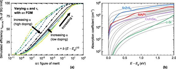
Figure 3. (a) The effect of varying α and τ on the maximum efficiency achievable by a simulated PV absorber. The average α (as defined in equation (1)) is varied by using different b values in the  expression. Thus, σ is constant in this figure. Different α values are represented by different colors, with darker colors indicating higher α values. When n is low, the ατ FOM is a fair descriptor of the maximum achievable efficiency, as found by Kaienburg et al [10]. When n is high, the ατ FOM is not appropriate. The other properties are fixed to their default values in table 1. (b) Comparison between the absorption coefficient spectra
  of four real PV absorbers (solid lines), and the hypothetical
  spectra defined by equation S10 and used to plot figure 4. These hypothetical spectra are among the ones that are employed when collecting the
  versus
  dataset used to develop the
  FOM. In real PV materials, a higher average α is often correlated with lower dispersion σ. This general trend guided the choice of the hypothetical
  spectra shown in (b).
Download figure:
Standard image High-resolution imageSimply setting n to a higher fixed value to simulate heavy doping ( ) radically changes this picture. As shown in figure 3(a), the different curves at constant α no longer line up. In particular, changing α from
  to
to  hardly has any effect on the efficiency at constant τ, as demonstrated by the one-decade horizontal shift between these two curves in most of the ατ range of interest. Hence, the ατ FOM appears to be approximately valid under the conditions simulated by Kaienburg et al but it may not be generalizable to other conditions.
3.2. Varying the dispersion σ of the absorption coefficient
To develop a new figure of merit step by step, I temporarily return to the initial assumption of  and let the dispersion of the absorption coefficient σ vary on top of α and τ. The different σ values are obtained by using the eight hypothetical
  spectra shown in figure 3(b) in the drift-diffusion simulations. These spectra have
  and
and  . See the supplementary Material for more details. Letting σ vary is a way to account for the diversity of absorption processes in the semiconductors that may be considered for the role of PV absorbers. Some features that influence the value of σ are direct versus indirect band gaps, different joint densities of states, different nature of optical transitions away from the band edges etc.
When σ is allowed to vary, the ατ FOM is no longer adequate (figure 4(a)) even in the limit of low doping density. Specifically, materials with a high σ like c-Si can only reach a substantially lower efficiency at constant ατ than materials with a low σ like chalcogenide perovskites. The problem with a high σ is that the carrier generation profile inside the absorber will be the sum of many exponentially-decaying profiles (corresponding to the different photon energies) with very different extinction depths. Thus, even if α remains constant, a thicker film is necessary to absorb the same fraction of the AM1.5G spectrum, resulting in a larger available volume for recombination.
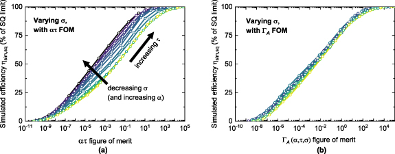
Figure 4. Development of the temporary  FOM by considering the effects of variable α, σ, and τ. (a) Simulated efficiency of PV absorbers with variable α, σ, and τ, plotted against the ατ FOM. Each color corresponds to a distinct (α,σ) pair, taken from the twelve hypothetical
  spectra in figure 3(b). Darker colors indicate higher values of α and lower values of σ. The different data points at constant (α,σ) are obtained by varying τ. (b) Same
  data as in (a), but plotted against the more predictive
  FOM defined in equation (8).
Download figure:
Standard image High-resolution imageTo incorporate the σ dependence, one can define a  FOM (A for 'absorption') as

where
and  . α and σ are in unitless form (see Methods section). The A1 factor is similar to the ατ FOM, with the addition of the σ−0.27 exponent to α, which extends its validity to different absorption coefficient dispersions σ. The A2 factor is an additional correction for the low ατ region, and it only 'turns on' when
  . If the same
  data points in figure 4(a) are plotted against the
  FOM (figure 4(b)), the points line up close to a single function. This demonstrates the appropriateness of
  when α, σ, and τ are allowed to vary and the other bulk properties are fixed to their default values in table 1.
3.3. Varying the doping density n
As we have already seen in figure 3, changing n can have a large impact on  . Figure 5(a) shows the effect of varying n between
  and
and  for two combinations of α and σ, while µ is still kept infinite. Clearly, modifications to the
  FOM are necessary to account for doping effects.
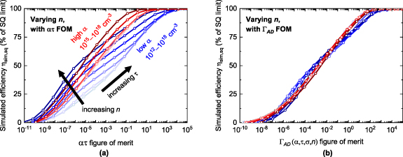
Figure 5. Development of the temporary  FOM by adding the effects of a variable doping density n to the
  FOM. (a) Simulated efficiency of PV absorbers with variable n for two distinct (α,σ) pairs (shades of red: high α and low σ; shades of blue: low α and high σ, see table 1). The data is plotted against the ατ FOM. Along each plotted line, ατ is varied by varying τ. The darkest colors represent
  . The lightest colors represent the doping density at which the curves start to overlap completely when n is decreased further (
 at high α,
  at low α). Between these extremes, n is varied by factors of 10. (b) Same
  data as in (a), but plotted against the more predictive
  FOM defined in equation (11).
Download figure:
Standard image High-resolution imageTo understand some of the trends, it is useful to consider the splitting of the quasi-Fermi levels (quasi-Fermi level splitting ( )) in an n-type absorber at open circuit under illumination. Under some assumptions [32]:

where  is Boltzmann's constant, T is the temperature,
  is the absorber's intrinsic carrier concentration and Δn and Δp are the excess carrier densities with respect to their equilibrium values in the dark (n and
  respectively). In many realistic scenarios, the QFLS equals the
  limit of a PV absorber [8, 33].
From equation (10),  (and therefore also
  ) are expected to rise logarithmically with increasing doping density when
  ('low injection' conditions) and be independent of doping density when
  ('high injection' conditions). This general trend is visible in figure 5(a). The transition between low- and high-injection conditions occurs at lower values of n as α is decreased, because Δn and Δp are lower due to the increased
  . In the low-α case, the transition shifts to higher n as τ is increased, because Δn and Δp become higher due to the lower SRH recombination rate. The slope change in the low-α curves at high n when
  is due to
  losses from incomplete light absorption (due to a low
  ) below this threshold.
It seems as if we could keep increasing the efficiency by increasing n to even higher values than  . However, several side effects can occur at very high doping density, such as a decrease of τ due to a higher density of recombination centers, a decrease of µ due to ionized impurity scattering, and an increasing weight of Auger recombination which is otherwise neglected in this study. In addition, the drift-diffusion simulation is no longer accurate because it relies on the Boltzmann approximation of the Fermi–Dirac distribution. This approximation breaks down at very high doping densities (see details in the supplementary material). Therefore, I do not consider doping densities above
  .
.
To account for the effects of different doping densities, the  FOM can be modified into the
  FOM (D for 'doping') as follows:

where
and  , d2 = 10,
  . α, σ and n are in unitless form (see Methods section).
According to the D1 factor, inclusion of doping effects in the FOM is important when  . For example, when
  low-injection conditions are realized when
  . When
  , low-injection conditions are realized when
  . The D2 factor is a correction for the high ατ region, as it only turns on when
  . The D3 factor is a additional correction for the low ατ region, as it only turns on when
  . The predictive quality of the
  FOM is shown in figure 5(b). The
  values line up near a single function when plotted against
  (figure 5(b)). This confirms the appropriateness of
  as a descriptor of
  when α, σ, τ, and n are allowed to vary and the other bulk properties are fixed to their default values in table 1.
3.4. Varying the carrier mobility µ
Allowing for finite values of the carrier mobility µ is a particularly important step, because the current generation of efficiency-prediction models based on the principle of detailed balance [5–9] still rely on the assumption of infinite mobilities. Thus, a method to estimate the maximum efficiency of candidate PV absorbers with finite mobilities would be highly desirable. Efficiency losses related to µ are mainly manifested in  and FF, because finite mobilities may lead to less-than-ideal carrier collection efficiency at voltages up to open circuit (figure 1).
In the study by Kaienburg et al [10] the relevant FOM changed from ατ to  when µ fell below the
  threshold. This threshold is, however, not a universal feature of a generic PV absorber, as demonstrated by varying µ between
  and
and  in figure 6(a). According to the figure, a
  threshold might be realistic only if n is low and the ατ product is so high that
  is close to the SQ limit for all but the lowest mobilities. In all other cases, the mobility threshold for a µ-dependent efficiency is higher, often by many orders of magnitude. Low mobilities are generally more tolerable if ατ is high and if n is low. When
  , even a very high mobility of
  is still below the threshold at low ατ products, and it has a detrimental effect on the efficiency (figure 6(a)). On the other hand, a mobility of
  is close to the threshold in the same ατ range when
  . These features can be understood on a qualitative level. As α increases, the optimal thickness of the absorber decreases, so carrier collection is facilitated. Hence, the requirements on µ are less stringent. As τ increases, the diffusion length (
 ) and the drift length (
 ) remain unchanged if µ decreases by the same amount [8].
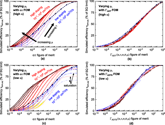
Figure 6. Development of two temporary FOMs ( and
and  ) to account for imperfect carrier transport. Transport-related losses are realized by varying the carrier mobility µ, which leads to less-than-ideal carrier collection efficiency and (mainly)
  and FF losses (figure 1). (a) Simulated efficiency of high-α PV absorbers with variable µ under high doping (shades of red) and low doping (shades of blue). See table 1 for the exact property values. The data is plotted against the ατ FOM. Along each plotted line, ατ is varied by varying τ. The lightest colors represent the lowest mobility of
  . From there, µ is incremented in factors of 10. The darkest colors represent the infinite mobility limit. (b) Same
  data as in (a), but plotted against the more predictive
  FOM defined in equation (13). (c) Simulated efficiency of low-α PV absorbers versus the the ατ FOM, with the same doping densities and lower mobility limits as in (a). The yellow-colored areas indicate scenarios where a low n yields higher efficiencies than a high n at the optimal thickness, everything else being equal. This corresponds to a drift-based solar cell with a wide depletion region being superior to a diffusion-based solar cell with a narrow depletion region [34]. Note that, at the lowest mobilities, the efficiency saturates to a value lower than the SQ limit, because the overall carrier lifetime cannot be increased beyond the radiative lifetime. To account for this saturation effect, the
  FOM, defined in equation (13), is developed. (d) Same
  data as in (c), but plotted against the
  FOM.
FOM.
Download figure:
Standard image High-resolution imageTo account for the effects of different mobilities, the  FOM can be modified to the
  FOM (T for 'transport') as follows:

where
and  ,
,  ,
,  ,
,  . All properties are in unitless form (see Methods section). Since µ only appears at the denominator of the T1 factor with an exponent of one, the
  FOM is directly proportional to µ when µ is well below a threshold defined by
  . This mobility threshold corresponds to

where all properties are again in unitless form. This analysis confirms that a linear dependence of the FOM on mobility (as in the simple  FOM by Kaienburg et al) is justified below a certain mobility threshold. Rather than being a constant universal value, the mobility threshold is a function of the other bulk material properties (equation (15)) and can vary by many orders of magnitude. The predictive quality of the
  FOM is shown in figure 6(b).
When a low µ and a low τ are combined with a low α (low efficiency region in figure 6(c)) a low doping density becomes more favorable than a high doping density. Although a higher n is still preferable to achieve a higher  (equation (10)), this effect is overcompensated by a
  improvement at lower n. The reason is that, when n is sufficiently low, an electric field is present throughout the absorber at short circuit due to full carrier depletion. The electric field adds a drift component to carrier transport, which improves the carrier collection efficiency and results in a higher
  with respect to the high-n case where transport mainly occurs by diffusion [34].
The µ-dependent simulations at low α (figure 6(c)) also reveal that  may saturate to a value lower than the SQ limit, even as τ keeps increasing (figure 6(c)). The reason why the SQ limit is never reached is that the diffusion length is ultimately limited by the radiative lifetime. Therefore, once the SRH lifetime has surpassed the radiative lifetime, the diffusion length can no longer be increased and
  remains constant even if τ is increased further [12]. If the diffusion length is smaller than the absorption depth due to an unfavorable combination of a low µ and a low α, the SQ limit is never reached. To take this effect into account in the FOM, the
  FOM can be modified to the
  FOM (S for 'saturation') as follows:

where
and  . All properties are in unitless form (see Methods section). The predictive quality of the
  FOM is shown in figure 6(d).
3.5. Varying the static dielectric constant ε and the DOS effective mass m
Varying the static dielectric constant ε of the PV absorber within two orders of magnitude ( ) has a weaker effect on
  compared to the other bulk properties examined so far (figure 7(a)). Neglecting possible indirect effects of ε on other properties (discussed later below), the main role of ε in a PV absorber is to modulate the width of depletion regions adjacent to the contacts, since ε enters Poisson's equation [35, 36]. The width of depletion regions may influence the diode ideality factor and the carrier collection efficiency [8]. Thus, changes in
  due to a varying ε are mainly due to
  and FF changes. Depletion region widths are proportional to
  , [36] so we may observe parallels between the effects of ε and the effects of n on
  and FF. As we have seen in the previous section, high values of n generally lead to a higher
  , with a low n being preferable only when µ, α, and τ are all low (figure 6(c)). Accordingly,
  increases with decreasing ε when µ is high, independent of the ατ product (figure 7(a)). The opposite trend is observed when µ is low and the ατ product is not too high. These results confirm again that narrow depletion regions (small ε) are generally preferable in 'good' PV absorbers (high
  product), whereas having wide depletion regions is more convenient in 'bad' PV absorbers (low
  product). The dependence of
  on ε weakens with decreasing n, because at sufficiently low doping densities the PV absorber may be fully depleted regardless of the value of ε. For an example, compare the curves with
  and
and  in figure 7(a).

Figure 7. The influence of the static dielectric constant ε and DOS effective mass m on the maximum efficiency achievable by a PV absorber. (a) Simulated efficiency of high-α PV absorbers with variable ε for high n (solid lines), low n (dashed lines), high µ (shades of red), and low µ (shades of blue). (b) Simulated efficiency of high-α PV absorbers with variable m for high n (solid lines), low n (dashed lines), high µ (shades of red), and low µ (shades of blue). See table 1 for the exact property values. The values of m shown in the plot are 0.12 m0, 0.54 m0, and 2.5 m0, with darker colors used for higher m values. In both subfigures, the data is plotted against the ατ FOM, and ατ is varied by varying τ along each plotted line. See table 1 for the exact property values.
Download figure:
Standard image High-resolution imageThe dependence of  on the DOS effective mass m of the PV absorber (figure 7(b)) is significant. This is expected, because m enters the expression for the QFLS (equation (10)). Thus, we expect that
  (the PV parameter directly related to the QFLS) should increase with decreasing m. Note that
  in equation (10), but the
  term is small compared to Δp under 1-Sun illumination so this additional dependence is negligible. The m-dependence of
  is stronger than its n-dependence, because the expression inside the logarithm in the QFLS expression (equation (10)) depends on
  under low injection conditions, and on
  under high injection conditions. Thus, the m-dependence is not affected by the carrier injection level. In figure 7(b), m is varied between 0.12 m0 and 2.5 m0. As expected,
  decreases with increasing m. For the high-mobility case—where equation (10) is valid—the efficiency indeed scales as
  , because the overlapping curves (solid and dashed red line) have roughly the same
  ratio (both n and m3 are changed by a factor 100). Note that the range of doping densities employed in figure 7(b) is sufficiently high to ensure low injection conditions (see also figure 5(a)).
The effect of both ε and m can be captured reasonably well by adjusting some of the factors in the  FOM expression in equation (16). However, since no new factors are needed when introducing these two new properties, the inclusion of variable ε and m in a FOM will only be shown in the next section as part of the final
  FOM including a variable band gap.
There is an important caveat regarding the effects of ε and m on PV efficiency. m and ε influence solar cell efficiency both directly (i.e. independent of the other bulk properties) and indirectly (i.e. by affecting the values of the other bulk properties, some of which explicitly depend on m and/or ε). As we have seen, the main direct effect of ε is on the width of depletion regions, [35] whereas the main direct effect of m is on QFLS (equation (10)). I emphasize that only direct effects are simulated in figure 7, because all the variable properties are independently changed in this study (see Methods section). However, both ε and m have substantial indirect effects [11, 32]. Some examples are given in the supplementary material. Importantly, many of these indirect phenomena affect the efficiency in the opposite direction of the direct effects modeled in figure 7. Hence, it is incorrect to draw conclusions such as 'increasing ε generally leads to lower efficiencies in the high-mobility limit' and 'increasing m generally leads to lower efficiencies' based on the trends in figure 7. This conclusion would only be true if changing ε and m did not affect the other properties.
3.6. Varying the band gap 

A very well-known effect of changing the band gap  of a PV absorber is modification of its SQ limit
  . Since calculation of
  is straightforward, this effect is taken into account by normalizing the simulated efficiency by
  , as done in most plots in this paper.
Plotting  data for absorbers with three different band gaps (figure 8(a)) demonstrates that normalization by
  is not sufficient to predict the efficiency of PV absorbers with variable band gaps via the
  FOM. This is not unexpected because
  enters the definition of many quantities that are relevant for PV efficiency. Examples are the QFLS (equation (10)), the intrinsic carrier density
  , the absorption coefficient spectrum
  , the generation rate, and the SRH recombination rate due to a mid-gap defect [8, 36, 37]. Interestingly, the
  FOM generally overestimates the efficiency potential of narrow band-gap absorbers and underestimates the efficiency potential of of wide band-gap absorbers (figure 8(a)), especially when
  is low. Due to the complex dependency between
  and
and  and the usage of a complex FOM in figure 8(a), this trend is not straighforward to rationalize. From further analysis of the simulated data, the trend seems to mainly be driven by the
  term in the QFLS expression in equation (10). If the excess carrier densities Δn and Δp only decrease weakly with increasing
  , then the QFLS is roughly equal to
  minus a positive constant. Hence, the QFLS becomes a larger fraction of
  as
as  increases, thus increasing
  for wide-gap absorbers.
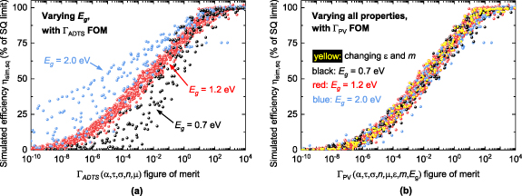
Figure 8. Development of the final  FOM to encompass PV absorbers with different band gaps, as well as the effects of different ε and m values shown in figure 7. (a) Simulated efficiency of PV absorbers with three different band gaps and various combinations of α, σ, τ, n, and µ. The plot of
  versus the
  FOM (equation (16)) demonstrates that
  is not an appropriate FOM for absorbers with band gaps significantly lower or higher than the 1.2 eV band gap used to develop the
  expression. (b) Same
  data as in (a) (with the addition of
  data from non-default ε and m values) plotted against the final
  FOM defined in equation (18). The data points with non-default ε and m values are identified by yellow markers. The
  FOM is generally predictive of the efficiency of PV absorbers in which
  , ε, and m are not fixed to single values.
Download figure:
Standard image High-resolution imageClearly, the  FOM must be extended to address the complex efficiency-band gap dependency. The outcome is the
  FOM as a function of all eight bulk properties in the
  set. This is the final FOM extension worked out in this article, corresponding to the end of Step B in figure 2. To develop the final
  FOM, I employ simulation data on absorbers with band gaps of 0.7 eV and 2.0 eV, while the other properties in the
  set are also varied. The rationale is to test a band gap range appropriate for PV absorbers that may be considered for single-, double- and triple-junction solar cells [38–40]. Note that many new simulated data points are employed for
  absorbers when developing the final
  , including other absorption coefficient spectra besides the ones shown in figure 3(b). This is done to check the robustness of the
  FOM and of the previously defined temporary FOMs.
I propose the following  FOM to include the effects of variable ε, m, and
  :
:

The various factors in equation (18) are defined as:


where all properties are in unitless form (see Methods section). The quantities  (
( ),
),  (
( ),
),  (
( ), and
  (
( ) are fixed parameters. Their values are given in the supplementary material. Note that
  contains new factors that were not present in the
  FOM. Also, most of the factors that were present in
  have been modified to generalize it to realistic ε, m, and
  ranges. To avoid confusion, I have then defined the factors of the
  FOM as
  ,
,  ,
,  ,
,  etc instead of as Ai
, Dj
, Tk
, Sl
etc. Since some of the fixed parameters have been adjusted as well, they are represented by barred lowercase letters in the
etc instead of as Ai
, Dj
, Tk
, Sl
etc. Since some of the fixed parameters have been adjusted as well, they are represented by barred lowercase letters in the  FOM, instead of as simple lowercase letters.
3.7. Estimating the maximum efficiency of a PV material from its FOM

We are now one step away from being able to estimate the maximum efficiency of a generic PV material from its  . The final step (step C in figure 2) is to find an appropriate function that gives a good fit to the
  versus
  data in figure 8(b). A temporary function that gives a fair fit (figure 9(a)) is the following:
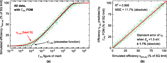
Figure 9. Prediction of the maximum efficiency achievable by a generic PV absorber through its  FOM (step C in the overall workflow in figure 2). (a) Fitting the entire
  dataset (2573 data points) versus
  . The piecewise function defined in equation (32) results in the efficiency estimate
  (dashed line), which is mainly of pedagogical value. A better fit is achieved by the function defined in equation (33). This function yields the efficiency estimate
  (solid line), which is used in the rest of the article. (b) Comparison between the maximum efficiency obtained by explicit drift-diffusion simulations (
 ) and the values predicted by the
  FOM through equation (33) (
 ).
).
Download figure:
Standard image High-resolution image
This piecewise expression is instructive, because it shows that the maximum efficiency approaches zero for very low values of  , and it approaches the SQ limit
  for very high values of
  , as expected from solar cell physics. For intermediate values of
  spanning eight orders of magnitude, the maximum achievable efficiency is proportional to the logarithm of
  minus a constant. A similar conclusion was drawn for the particular case of the ατ FOM [10].
The piecewise expression in equation (32) does not give a good fit in the  region (figure 9(a)). To predict efficiency limits as accurately as possible, I propose the following function instead:
The three ki
terms are fixed parameters, with their values given in the supplementary material.  is simply equal to
  . The expression proposed in equation (33) gives a good fit to the
  versus
  data (figure 9(a)), with
  and a mean squared error of 11.7% absolute (figure 9(b)). Assuming that
  , we can conclude that the
  FOM enables immediate prediction of the maximum efficiency of a generic PV absorber with an absolute error of
  on the fraction of the SQ limit. As an example, we can estimate the maximum efficiency achievable by the hybrid perovskite absorber CH3NH3PbI3 (MAPI) with a band gap of 1.55 eV and a set of bulk properties typical of its current state of the art, as given in table 2. MAPI is a convenient material for this analysis because it is structurally isotropic, so its properties do not have a strong direction dependence. Furthermore, τ, µ and m in MAPI have similar values for electrons and holes, [21, 43, 47] so the definitions of the
  set proposed in the methods section is rather unambiguous.
Table 2. Best guesses for the values of the eight properties in the  set exhibited by CH3NH3PbI3 (MAPI) films used to fabricate state-of-the-art MAPI solar cells with power conversion efficiency up to 21.3
 . The SQ limit
  of MAPI is given, together with the maximum efficiency predicted for MAPI films with these specific property values as a fraction of the SQ limit (
 ), and as absolute power conversion efficiency (
 ).
).

| α | τ | µ | n | m |

|

|

| |||
|---|---|---|---|---|---|---|---|---|---|---|---|
| (eV) | (cm−1) | σ | (s) | (cm2 V−1s−1) | (cm−3) | ε | (m0) | (%) | (% of  ) ) | (%) | |
| MAPI | 1.55 [41] |
 [42] [42] | 0.63 [42] |
 [43] [43] | 10[44] |
 [45] [45] | 33.5 [46] | 0.15 [21] | 31.4 |

|

|
The efficiency limit derived by substituting MAPI's specific  set (table 2) into equation (33) is
  of its SQ limit of
  . This corresponds to a maximum power conversion efficiency of
  , a few percent better than the highest efficiency I am aware of (21.3%) for a pure MAPI absorber without alloying [48]. The main message is that device-level improvement may help improve efficiencies in MAPI solar cells up to the
  limit, but bulk property improvement in MAPI films is likely necessary to exceed this limit. Importantly, we can also estimate the efficiency potential of a hypothetical 'bad' MAPI sample with the same properties as state-of-the-art samples, except for a lower carrier lifetime τ = 10 ns. The corresponding efficiency limit is
  . If, in addition, the mobility of the 'bad' sample is also lower than its state-of-the-art value (say
  ), the efficiency limit further drops to
  .
.
4. Discussion
To assess the quality of a PV absorber through its  FOM and the corresponding efficiency potential
  , the eight bulk properties in the
  set must be known for that specific material. All the eight properties are—in principle—experimentally accessible for any PV absorber in thin-film form without the need to fabricate a complete device. Thanks to recent advances, [49, 50] these properties are now also accessible via first-principles electronic structure calculations, albeit at various degrees of computational expense and accuracy. A more detailed discussion is available in the supplementary material. Absorbers exhibiting a strong carrier-type- or direction-dependence in their properties create some ambiguity in the choice of the values to be used to calculate the FOM. Some preliminary suggestions to derive (single) effective values for these properties are given in the supplementary material.
Predicting maximum PV efficiencies via the  FOM has some advantages with respect to using detailed-balance methods based on generalization of the SQ limit to account for non-radiative recombination [6–9]. Such methods deduce efficiency limits based on fundamental physics. While they are intrinsically more exact, deduction of efficiency limits for the case of finite mobilities and finite depletion region widths has proved elusive until now. Thus, possible negative effects of µ, ε, and n on (especially)
  and FF are omitted. On the contrary, efficiency predictions via the
  FOM are based on induction, i.e. by generalization from a large number of observations. This makes it possible to develop an FOM expression independently of the underlying physics. The positive outcome is that the effects that are neglected by deductive methods can be included. Since these effects have a negative influence on
  , the
, the  efficiency limit set by the FOM is stricter than for deductive methods, and it gives a fairer assessment of low-mobility materials in particular. In addition, the
  limit can immediately be calculated from a single explicit equation unlike the case of deductive methods, where the optimal thickness first has to be determined through an iterative procedure.
We have already seen in figure 3(a) that the  FOM approximately reduces to the simple ατ FOM proposed by Kaienburg et al [10] as long as the property ranges are within the limits explored by the authors and µ is sufficiently high. Such ranges are only a limited subset of the conditions sampled in the present study. The ατ FOM is found to be invalid under most conditions that do not match the ones simulated by Kaienburg et al even under the assumption of infinite mobilities (see figures 4, 5 and 7). The inclusion of the ατ as a special case of
  is further discussed in the supplementary material. Similarly, the
  FOM approximately reduces to the
  FOM, as long as the property ranges are within the limits explored by Kaienburg et al and µ is sufficiently low. The inclusion of the
  as a special case of
  is also discussed in more detail in the supplementary material. Finally, the mobility threshold where
  becomes µ-dependent is not a universal value, but is a function of the other bulk material properties, as shown by equation (15). This threshold can vary by many orders of magnitude in different PV absorbers with realistic values of their bulk properties.
5. Outlook
Even though the  FOM can be a powerful tool for PV materials research, a number of future developments would be desirable. First, the validity limits of
  should be tested more systematically. Although I have made an effort to choose a diverse
  dataset for deriving
  , the current FOM expression (equation (18)) may be inaccurate for some
  combinations that fall within the sampled range in table 1, but that are not included in the ∼3000 particular combinations making up the training set. On the other hand, it is not implausible that
  may remain sufficiently accurate even when some of the properties fall outside the ranges in table 1.
Second, there is no guarantee that the current expression of  is the simplest possible definition to achieve the present level of accuracy and generality. It may be possible to simplify or fully redefine some factors in
  without significant differences in the final numerical result. Even though the roles of the different
  factors in equations (19)–(31) have been physically rationalized when possible, their expressions were still chosen on a phenomenological basis and might not be the most physically insightful. Searching for alternative expressions of the FOM factors that can be more easily related to known solar cell physics would be desirable.
Third, the  FOM is a predictor of PV efficiency only. A prediction of the corresponding
  ,
,  , FF, and optimal absorber thickness would also be useful. Deductive methods can only predict these parameters in the limit of perfect carrier collection, so this problem remains open.
Fourth, a major assumption in this study has been that the eight bulk properties included in the  FOM do not influence each other. In reality, there are many interdependencies between these properties. For instance, increasing m will generally lead to lower σ and µ [32]. Increasing ε is likely to give higher τ and µ [11]. Hence, in a more complete treatment of the problem, the eight properties would be written as a function of the other properties that may influence their value. This is not a trivial task, because the relationships between the different properties cannot generally be written as simple functions.
Finally, the development of the  FOM has relied on numerous other assumptions, as detailed in the Methods section. In particular, the FOM only applies for planar single-junction cells obeying the SQ limit. Further, absorbers exhibiting a strong carrier-type- or direction dependence in their properties create some ambiguity in the choice of the values to be used to calculate the FOM. Relaxing one or more of these assumptions (and redefining the
  FOM accordingly) will probably improve its generality.
The approach taken in this study (figure 2) has been to generate a training dataset from drift-diffusion simulations, and to develop  from trends in this dataset using human intelligence. This methodology is a hybrid between a fully physics-centered approach where very little data is necessary (e.g. deductive methods) and a fully data-centered approach where very little or no physics is necessary (e.g. artificial intelligence). An advantage of the hybrid approach is that some of the strengths of the two extremes are retained. Basing the FOM development on an extensive training data set facilitated work in an eight-dimensional property space, allowing for generalization of
  . On the other hand, the human element made it possible to write an explicit mathematical relationship between efficiency and bulk material properties, allowing for interpretation and comparison to simpler FOMs.
In spite of these advantages, moving to either a more physics-centered or a more data-centered approach may be a sensible strategy for addressing some of the remaining challenges listed above. Generating a more extensive drift-diffusion simulation dataset and using it as a training set for machine learning techniques may improve accuracy and generality. An obvious choice for the features to be used in a machine learning model are simply the eight properties in the  set. Once an appropriate machine learning model is developed, separate predictions of
  ,
,  , FF, and optimal absorber thickness may turn out to be a straightforward task.
More physics-centered approaches to FOM development could take two paths. The first is to extend the current state-of-the-art, detailed-balance-based deductive methods to the case of imperfect carrier collection. The second is to define the different terms in  by including parameterized expressions of known quantities that are known to play a role in solar cell physics (such as the diffusion length, drift length, depletion region width, excess carrier density, etc), and then fit the parameters to the training dataset.
6. Conclusion
I have proposed a phenomenological expression (equation (33)) for the efficiency limit  of a generic PV material as a function of its SQ limiting efficiency
  and of eight of its bulk material properties (table 1). These properties build up a global FOM
  (equation (18)), which can be used to evaluate the overall quality of any PV material at any stage of development. The eight material properties are all experimentally accessible and, with some caveats, can also be calculated by first-principles electronic structure methods. Thus, the efficiency limit is applicable both to synthesized materials and to computationally screened materials. For intermediate values of
  , the efficiency limit is approximately equal to
 ![$\left[\frac{1}{8} \text{log}(\Gamma_{\mathrm{PV}})+\frac{3}{4}\right]\eta_\mathrm{sq}$](https://content.cld.iop.org/journals/2515-7655/6/2/025009/revision2/jpenergyad2499ieqn461.gif) (equation (32)). As expected, the efficiency approaches zero and
(equation (32)). As expected, the efficiency approaches zero and  for very low and very high values of
  , respectively.
The efficiency limit  set by the
  FOM is more stringent than corresponding limits set by deductive methods based on the principle of detailed balance. The main reason is that efficiency losses by imperfect carrier collection (primarily influencing
  and FF) are taken into account in
  by including the µ and ε material properties. The previously proposed ατ and
  FOMs are found to be special cases of the more general
  FOM.
FOM.
Acknowledgments
I welcome comments, critiques, extensions, and justified corrections to the FOM proposed here. This work was supported in part by a research Grant (42140) from VILLUM FONDEN and co-funded by the European Union (ERC, IDOL, 101040153). Views and opinions expressed are however those of the author only and do not necessarily reflect those of the European Union or the European Research Council. Neither the European Union nor the granting authority can be held responsible for them.
Data availability statement
The data that support the findings of this study are openly available at the following URL/DOI:https://doi.org/10.11583/DTU.24894933.
Supplementary data (2.9 MB PDF) Additional methods; determination of bulk properties; relationships between properties; comparison between present FOM, earlier FOMs, and detailed balance methods; values of drift-diffusion simulation parameters; values of fixed FOM parameters.