

Abstract
Slow acquisition time and instrument stability are the two major limitations for the application of confocal Brillouin microscopy to biological materials. Although overlooked, coupling the microscope to the spectrometer with a multimode fiber (MMF) is a simple yet viable solution to increase both the detection efficiency and the stability of the classical single-mode fiber-coupled virtually imaged phase array (VIPA) instruments. Here we implement the first successful MMF-coupled VIPA spectrometer for confocal Brillouin applications and present a dimensioning strategy to optimize its collected power. The use of an MMF brings a tremendous improvement on the stability of the spectrometer that allows performing experiments over several weeks without realignment of the device. For instance, we map the Brillouin shift and linewidth in growing ductal and acinar organoids with a spatial resolution of  and
and  dwell time. Our results clearly reveal the formation of a lumen in these organoids. Careful examination of the data also suggests an increase in the viscosity of the cells of the assembly.
Export citation and abstract BibTeX RIS

Original content from this work may be used under the terms of the Creative Commons Attribution 4.0 license. Any further distribution of this work must maintain attribution to the author(s) and the title of the work, journal citation and DOI.
1. Introduction
The mechanical properties of cells and tissues have been recognized as key players in myriads of physiological processes such as growth [1], morphogenesis [2], migration [3], and their alteration is involved in several pathologies like cancer [4] or neurodegenerative diseases [5]. At the cellular scale, many techniques have been developed to probe the mechanics (stiffness, viscosity, adhesion ), mostly based on contacting probes (e.g. atomic force microscopy, magnetic tweezers cytometry and micropipette aspiration) or the tracking of fluorescent markers. At the tissues scale, contact-based techniques are limited to near-surface characterization, and diffusion and absorption limit the depth at which fluorescent tags can be quantitatively imaged in live samples.
In recent years, a new microscopy technique based on the scattering of light by thermally induced mechanical vibrations—called Brillouin light scattering (BLS) [6, 7]—has been introduced in biology. The analysis of the spectrum of the scattered light allows retrieving the propagation parameters of acoustic waves (sound velocity and attenuation) in the sample, thus enabling the characterization of its high-frequency mechanical properties [8]. This all-optical, non-contact technique allows quantitative imaging in cells and tissues, offering many applications in biology [9, 10] with an appeal however mitigated both by the long-term stability of the instruments and the extended acquisition times.
Advances in instrumentation have led to the introduction of the VIPA spectrometer in 2008 [11], a simple yet effective instrument that has fostered investigations of diverse biological samples among which biofilms [12], cells [13, 14], organoids [15], and zebrafishes [16, 17]. For biological imaging, it is usual to combine the VIPA spectrometer with a confocal microscope. This approach optimizes spatial resolution but restricts the light flux from the sample. Various techniques have been proposed to increase the acquisition speeds of Brillouin spectra. These techniques either aim at changing the way we illuminate the sample so as to increase the energy of the scattered light, for example using stimulated Brillouin scattering [18] or to observe more than one point in the sample per scan, for example using light-sheet Brillouin spectroscopy [19].
Here we propose to use BLS to image the morphogenesis of submillimeter organoids. Organoids are in-vitro 3D multicellular biological models obtained from cells self-organizing in three dimensions. They recapitulate at least partially the organization and properties of the tissues from which they derive and are therefore valuable research models for studying normal or pathological tissue development. They offer an invaluable tool for investigating tissue development [20] and are expected to be used in various medical applications, including drug discovery [21] and personalized medicine [22]. In this study we consider ductal or acinar organoids: they are spherical in shape, with a central hollow lumen enveloped by a layer of peripheral cells. In these tissues, the occupancy of the luminal space often serves as a marker of pathology, with potential implications in oncogenesis [23]. Consequently, investigations performed on acinar or ductal organoids regularly involve a meticulous monitoring of their morphology by an expert observer using brightfield microscopy. Such studies are resource-intensive, inherently restricted in size, and remain subject to interpretation.
In this context, we propose to use BLS images for high-throughput monitoring of the luminal space. To achieve this we optimize the spatial resolution and the collected light flux by carefully dimensioning the confocal microscope. A confocal microscope differs from a classical microscope by focusing the captured light onto a finite-size aperture referred to as the confocal pinhole [24]. The size of this confocal pinhole is paramount in the system as it regulates both the spatial resolution of the instrument and its signal-to-noise ratio (SNR) [25, 26]. In BLS spectra, the wavelength distribution of the noise is essentially that of the illumination. Therefore, if we can fully extinguish the illumination wavelength outside the confocal microscope, enlarging the pinhole should reduce the spatial resolution but increase the signal intensity, thereby increasing the speed of the measurement.
The ability to couple light inside the pinhole is therefore the limiting factor for this approach. This is especially limiting when using optical fibers in place of the pinhole, as is classically done in BLS microscopy. In this case, a limit on the effective confocal pinhole size depending on the number of modes a fiber can carry appears [27, 28]. In this study, we therefore propose to rely on an multimode fiber (MMF) rather than an single-mode fiber (SMF) to overpass this limitation. By doing so we expect to improve the throughput of the instrument, but also easier alignment of the device and better stability to mechanical vibrations in experimental conditions.
The use of MMF-coupled VIPA spectrometers has only recently been proposed for astronomical measures [29] and is new to the field of BLS. For this application however, this design poses a real challenge in terms of efficiency of the device: the use of an MMF rather than an SMF drastically increases the size of the beam inside the spectrometer, which in turn potentially affects the coupling efficiency of the light inside the VIPA étalon, as previously noted by Meng and Yakovlev [30]. This coupling efficiency has however never been studied in the literature to our knowledge, and the results from Zhu et al [29] suggest that small core MMFs could perform as well as SMFs in VIPA spectrometers. Therefore, we here propose to quantify this coupling efficiency and build an MMF-coupled VIPA spectrometer. We will characterize both its response and the acquisition speed it allows. For demonstration, we will study the development of growing acinar and ductal organoids during their morphogenesis. We will focus in particular on the growth and mechanical properties of the lumen.
2. Materials and methods
2.1. Spectrometer
The instrument used in this study is a one-stage VIPA spectrometer working at  using a rubidium cell to filter out the elastically scattered light from the signal, as previously presented in the literature [31]. It essentially differs from previous instruments on two key aspects: the use of an MMF to carry the light from the confocal microscope to the spectrometer, and the presence of two telescopes before and after the rubidium cell to reshape the beam.
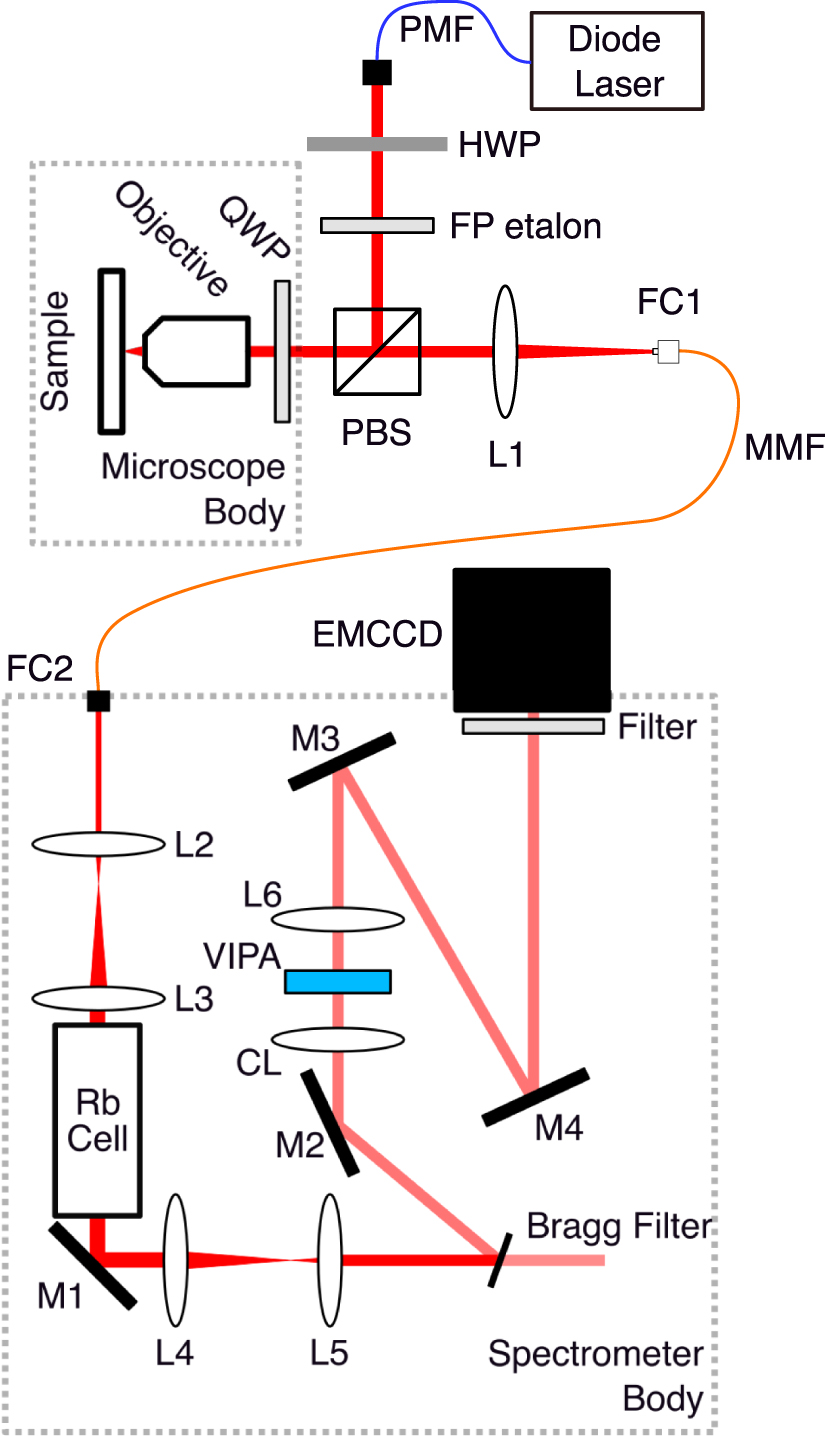
We schematize in figure 1 the actual arrangement of the device. A single-frequency  linearly polarized fibered laser diode (Sacher Lasertechnik Micron) is coupled to a fiber collimator (Thorlabs F280FC-780,
  ) chosen to fill the pupil of our objective. The laser is then passed through a tilted Fabry–Pérot étalon to reduce the amplified spontaneous emission level of the laser to an expected
  at
at  from the central peak of our laser. The power of the illumination measured at the sample plane was typically
  .
.

Figure 1. Schematic view of the experimental setup. PMF: polarization maintaining fiber, MMF: multimode fiber, FC1-2: fiber coupler, FP: Fabry–Pérot, HWP: half-waveplate, PBS: polarizing beam splitter, QWP: quarter-waveplate, L1-6: spherical lenses, CL: cylindrical lens, M1-4: mirrors, Rb cell: rubidium cell.
Download figure:
Standard image High-resolution imageWe adjusted the beam polarization with a half-waveplate before directing it with a polarizing beam splitter (PBS) to a quarter-waveplate (QWP) and then, a microscope. We used a 50× objective with 0.65 numerical aperture (NA) (Olympus LCPLN50XIR) to focus the beam on the sample. We collected the backscattered light with the same objective and, after readjusting its polarization with a QWP, we directed it with the PBS and then coupled it into an optical fiber.
We used a  lens (Thorlabs LA1131-B) to focus the beam into an MMF with a core diameter of
  and a 0.1 aperture (Thorlabs M67L02). In this configuration, the core of the fiber measured with respect to the diffraction spot, is
  , where an Airy Unit (AU) defines the diameter of the diffraction spot . We assessed the experimental axial resolution by a knife-edge experiment and found an axial resolution of
  (see supplementary information), which would correspond to an effective confocal pinhole size of
  . We attribute this difference between data and prediction to uncertainties in the specifications of the optical components used.
The fiber is then coupled to the VIPA spectrometer through a fiber collimator (Thorlabs F280FC-780,  ). The beam is shaped to fill the diameter of a rubidium cell (Sacher Lasertechnik VC-Rb-19x75-Q) used to absorb the backscattered light at the laser's wavelength [31, 32]. The minimal extinction of the rubidium cell was measured at
  for a single pass and a path length of
  . In this configuration, in absence of saturation of the cell, the intensity of the elastically scattered light was smaller than the noise floor of the instrument. The beam is then shaped to be filtered by a narrow (
 ) Bragg filter (Ondax NoiseBlock) centered on the laser frequency and analyzed by a one-stage VIPA spectrometer. The Bragg filter is used to filter out the ASE that is not filtered by the étalon.
The spectrometer is composed of a  cylindrical lens (Thorlabs LJ1653RM-B), a fused-silica VIPA étalon with
  FSR (Light Machinery OP-6721-3371-4), a
  spherical lens (Thorlabs LA1380-B) and an EMCCD camera (Andor iXon Ultra) presenting a detector size of
  pixels and a pixel size of
  . The VIPA tilt angle is set to approximately 2∘ to allow three interference orders to be visible on the detector. In this configuration, the transmission of the spectrometer is measured to be 35%, which is lower than the 55% transmission values reported for other SMF-coupled VIPA spectrometer configurations [33], and the 56.9% transmission reported by Zhu et al when using the same optical fiber in their setup [29]. We therefore attribute our reduced transmission to the compromises we made in the choice of the optics, the quality of the alignment and the combined effect of the size of the beam that enters the VIPA étalon and the non-idealities of the VIPA.
In this configuration, the spectral resolution is  , obtained by fitting a Lorentzian curve to the experimental response of the spectrometer to the laser. This value is in good agreement with the manufacturer's data for the finesse of the VIPA etalon (50) and free spectral range (
 ). This shows that the use of an MMF induces no broadening effects. We also placed a narrow-band optical filter (Semrock 785 nm MaxLine) before the detector to remove any ambient light that might enter the spectrometer's body.
The Brillouin peaks observed in the spectrum of the scattered light are linked to the optical and acoustic properties of the material by the following equations [34]:
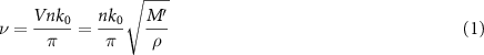

where V, n and α are the average sound velocity, average refractive index and average sound attenuation in the volume observed, k0 the wave vector of the incident light, respectively. ν and Γ are the frequency shift with respect to the incident light and linewidth of the scattered peaks, respectively. M is the complex longitudinal modulus (real part M', and imaginary part M''). ρ is the average density in the volume observed. Equation (1) is valid in backscattering geometry.
2.2. Hardware control and data analysis
The locking of the laser wavelength on the rubidium cell's absorption line is a well-documented issue. In our setup, this issue further extends to the precise and stable locking of the étalon used to attenuate the ASE on the laser's wavelength. To tackle these issues, we developed a dedicated Python software to dynamically adjust the tilt of the étalon and the laser frequency in real-time. The tilt of the étalon is slightly adjusted every 5 min with steps of approximately 0.0005∘ using a piezoelectric mirror mount, in order to obtain the highest transmission of the laser through the étalon. This same software controls the movement of the microscope stage and the trigger of the Electron Multiplying Charge-Coupled Device (EMCCD), allowing the acquisition of BLS spectra in all three dimensions of the sample. Because the samples evolve and therefore move between two different measures, we took care for this study, to manually reposition the sample with respect to the microscope's objective before each acquisition.
We used a complementary Python program to extract and analyze the data. This program uses the method described by Wu et al [35] to obtain a frequency axis for a spectrum. It then relies on a Lorentzian fit to estimate the values of Brillouin shift and linewidth for the given spectrum. Figure 2 shows the Brillouin scattered spectrum obtained inside an organoid (in plain blue lines) where each Brillouin peak is fitted with a Lorentzian function (in dashed red lines). The good agreement between the experimental lineshape and the function lineshape justifies here our choice of a Lorentzian function to fit the spectra. This treatment ultimately returns arrays of shift and linewidth values for each sample, that can be either used for further treatment or displayed in the form of images, using the values for Brillouin shift or linewidth as contrast.

Figure 2. Typical Brillouin spectrum obtained with our multimode-fibered VIPA spectrometer inside an organoid (blue line) fitted with Lorentzian functions (red dashed lines). The inset is a zoom on the anti-Stokes Brillouin peak of the central order of interference.
Download figure:
Standard image High-resolution image2.3. Cell culture and imaging protocol
We used two different models of ductal and acinar organoids in this study, respectively: pancreatic organoids derived from the pancreatic cell line H6c7 and prostatic organoids derived from the prostatic cell line RWPE-1. We first confirmed our ability of recognizing morphological traits of multicellular assemblies with BLS on fixed H6c7 organoids and then followed the development of live RWPE-1 organoids with BLS during their morphogenesis.
H6c7 cells were trypsinized, counted and seeded onto a Matrigel® bed. Plates were incubated for  at
at  for cell sedimentation. Top coats obtained by adding 4% Matrigel® in cold keratinocytes serum free medium (SFM) medium (Thermo Fisher) supplemented with 5% fetal bovine serum (FBS) and 5 ng ml−1 epidermal growth factor (EGF) were subsequently gently added on top of the cells. Plates were then incubated for 9 Da, with a change of medium after one week of culture. The resulting organoids were finally fixed to be used as time-invariant samples and stored at
  .
.
RWPE-1 cells were trypsinized, counted and seeded onto a Matrigel® bed. After cell sedimentation, a top coat composed of 10% Matrigel® in cold keratinocytes SFM medium supplemented with 2% FBS and 20 µg ml−1 EGF was gently added on top of the cells. The assemblies developed in a microscope incubator at  ,
,  and 100% humidity, allowing the monitoring of their morphogenesis using BLS without affecting their development. The medium of the samples was changed after the first
  of culture and every week after to ensure correct development of the structures. The assemblies were finally compared with a control plate stored in a dedicated incubator to guarantee that our measure did not influence the development of the structures.
In the case of H6c7 organoids, the imaging was done on fixed tissues. In the case of RWPE-1 organoids, live tissues where imaged.
3. MMF-coupled VIPA spectrometer
3.1. Theoretical arguments for the coupling of multimode beams in VIPA étalons
Spectrometers used for Brillouin scattering applications require both high resolving power and high spectral dispersion. In the context of VIPA spectrometers, these characteristics practically impose the use of thin VIPA étalons tilted at small angles, which in turn constrain both the size and the divergence of the beam of light coupled to the VIPA. This constraint is schematized in figure 3(a) where, for a given tilt angle of the VIPA, we geometrically establish a link between the convergence of a beam and its size at focus. The product of the surface S of a beam and its solid angle  , where NA defines the NA of the beam, is used in the definition of the so-called étendue
 [36], where n is the refractive index of the medium of propagation of the beam. We therefore add on figure 3(a) qualitative vision of the étendue for different coupling configurations. As a configuration giving a non-zero coupled étendue exists, a maximum of coupled étendue also exists for a given VIPA étalon tilted at a given angle (see analytical description in supplementary information).
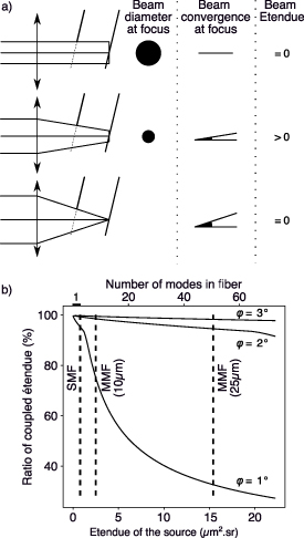
Figure 3. Geometrical study of the coupling of light in a VIPA studied for sources of different geometrical étendues. (a) For a given étalon tilted at a given angle, representation of three coupling configuration together with the size at the beam at focus, the convergence of the beam at focus and the resulting coupled étendue. (b) Allowing part of the étendue to be rejected, ratio of the beam étendue coupled inside the VIPA étalon as a function of the geometrical étendue of the source when the convergence of the beam coupled in the VIPA étalon matches the tilt of the VIPA étalon. ϕ defines the tilt angle of the étalon, SMF stands for 'Single mode fiber' and 'MMF' for multimode fiber.
Download figure:
Standard image High-resolution imageIn a lossless system, the étendue of a beam is an optical invariant [37]. Therefore, if the source of the signal presents an étendue larger than the maximum defined by the tilt of the étalon, part of the signal will be lost due to the coupling of the beam inside the VIPA étalon. For a multimode optical fiber, the notion of étendue can be linked to the number of modes the fiber carries  , through its 'waveguide parameter' (also commonly referred to as the 'V-number' of the fiber). The waveguide parameter can be computed using:
  , where
  and
and  define respectively the area of the core of the fiber and the NA of the fiber. We can therefore approximate the number of modes carried by the fiber by
  . As such, we can therefore think that the more modes an optical fiber carries, the less effective the coupling of the beam it carries inside a VIPA étalon. However, when considering an étalon tilted at 2∘, a value usual for VIPA spectrometers applied to BLS [38, 39], the maximal, optimally coupled étendue can be computed and is equal to
  . For a Gaussian beam, the étendue being usually approximated by λ2, we could in theory couple more than 15 times the étendue of an SMF inside the VIPA. Consequently, we can theoretically couple more than the étendue corresponding to an SMF inside a VIPA étalon, therefore use MMFs, without compromising the coupling efficiency of the beam inside the VIPA, in a configuration that allows for the analysis of a BLS spectrum.
This approach theoretically supports the idea of using MMFs in VIPA spectrometers but when looking at the condition it fixes on the beam, we see that it can encourage the use of small convergence angles inside the étalon, which raises issues when dimensioning the instrument. Reasoning therefore on the coupling efficiency of a beam of given étendue, with an angle of convergence inside the VIPA étalon equal to the tilt of the VIPA (see supplementary information for calculation details), a configuration much closer to experimental configurations, we can then study the coupling efficiency inside the étalon. Figure 3(b) displays for different angles of tilt of the VIPA étalon close to 2∘, the coupling efficiency of a range of beam as a function of their étendue. In order to clarify this representation, we add on top axis the number of modes supported by a fiber that outputs a beam of the given étendue. We also add on this figure, in dotted lines, the étendue of a beam supported by three commonly accessible optical fibers working at  : an SMF, a
 MMF and a
 MMF. This figure shows that the coupling efficiency diminishes with the étendue of the beam, and that the smaller the tilt angle of the VIPA, the greater the impact on the coupling efficiency. Note that this figure also suggests the possibility of increasing the tilt angle of the VIPA étalon to increase the coupling efficiency of large étendue beams, and therefore large étendue MMFs. This solution can be interesting for applications where the spectral dispersion can be reduced however it is impractical for Brillouin scattering applications, as previously noted by Meng and Yakovlev [30].
More importantly, we see on figure 3(b) that for small étendue MMFs (
 MMF and a
 MMF), the coupling efficiency remains essentially equal to the one of an SMF, without compromising the dimension of the whole instrument. Therefore by using a
 MMF in the VIPA spectrometer, we essentially increase the étendue of the beam we observe by more than one order of magnitude. For studying extended sources of light, for which the luminance L can be considered homogeneous, using an MMF therefore allows an increase of more than one order of magnitude in the optical flux Φ, as the flux can be defined as the product of the luminance of a beam by its étendue:
  . The use of MMFs in VIPA spectrometers therefore is of particular interest in astronomical applications.
3.2. Theoretical benefits of using MMFs in confocal VIPA spectrometers
In the context of confocal BLS, we use a confocal microscope to collect the light. Hence the collected light flux is solely defined by the the confocal pinhole size, taken with respect to the figure of diffraction [25]. When we replace this pinhole by an optical fiber, a condition on mode coupling appears, and results in the existence of a maximum in collected light flux for a confocal pinhole size, taken with respect to the figure of diffraction. For instance when using an SMF, this 'optimal pinhole' radius can be approximated to 1.6 optical units [27] or, when expressed in AU, an 'optimal pinhole' diameter of 0.84 AU. Using an MMF is therefore a way to increase the 'optimal pinhole size' of the confocal microscope over this value, and therefore improve the signal level of the instrument. In order to quantify this improvement, we propose to evaluate the collected power,  . To do so, we write the scattered Brillouin power
  at a slice of thickness dz located at the height z:

where  is the Brillouin cross-section by unit volume,
  the laser power at a depth z and
  is the solid angle seen by the objective.
We can obtain in this description, the total collected power by integrating the scattered power on all the object volume. We can consider in this object space, the distribution of laser to be Gaussian. If we write  the linewidth of this distribution, then the collected power
  writes (see details in supplementary information):

where  is the laser power when collimated.
Using the expression of  given by Wilson [40], we obtain:

where  is the diameter of the confocal pinhole normalized to the diffraction spot size, given in AU.
Table 1 presents a few examples of configurations where different objectives are used in combination with different pinhole sizes, given in AU. This table compares for different configurations, the axial and transverse resolution predicted by confocal microscopy theory, as well as the expected collected power. As only the aperture of the objective, the refractive index of the medium of propagation of the light and the pinhole size affect the spatial resolution of the instrument, we choose to normalize the power collected so as to only consider the effect of these parameters. We therefore use the following expression for the normalized collected power: ![$P_\mathrm{col, normalized} = \mathrm{NA}^2/\left[n - \sqrt{n^2-\mathrm{NA}^2}\right]\sqrt{1+v_\mathrm{AU}^2}$](https://content.cld.iop.org/journals/2515-7647/6/2/025010/revision3/jpphotonad378cieqn62.gif) .
.
Table 1. Comparison of different confocal microscopy configurations for confocal Brillouin scattering measurements. The power has here been normalized to only assess the influence of the refractive index n, the aperture of the objective NA and the size of the pinhole given with respect to the diffraction spot  . We highlight our configuration in bold font.
| Objective (M, NA) | Pinhole size (AU) | Spatial resolution ( × ×  ) ) |
 (norm.) (norm.) |
|---|---|---|---|
| 5×, 0.1 | 0.5 |

| 2.23 |
| 1.5 |
| 3.60 | |
| 3 |
| 6.31 | |
| 10×, 0.3 | 0.5 |
| 2.18 |
| 1.5 |
| 3.52 | |
| 3 |
| 6.18 | |
| 20×, 0.45 | 0.5 |
| 2.12 |
| 1.5 |
| 3.41 | |
| 3 |
| 5.99 | |
| 50×, 0.65 | 0.5 |
| 1.97 |
| 1.5 |
| 3.17 | |
| 2.5 (ours) |

| 4.73 | |
| 3 |
| 5.57 |
We see that we can optimize  in the fiber-coupled VIPA spectrometer given a spatial resolution by using a high NA objective with a large pinhole size rather than a small NA objective used at the limit of diffraction. Note that this strategy is technically applicable both for the SMF and MMF-coupled VIPA spectrometer. However due to the losses induced by mode-coupling, for large pinhole sizes, and therefore the larger collected flux, it is only interesting when using MMFs.
In the context of our study, for an instrument with a spatial resolution of  , we can essentially choose between two different configuration:
- A confocal VIPA spectrometer that uses a 20 ×, 0.45 NA objective and a
 confocal pinhole, thus allowing the use of an SMF. This instrument presents a spatial resolution of .
 - A confocal VIPA spectrometer that uses a 50 ×, 0.65 NA objective and a confocal pinhole, thus only interesting when using an MMF in a fiber-coupled device due to the limitations brought by mode coupling. This instrument presents a spatial resolution of


These two instruments are equivalent in terms of spatial resolution. Following the work of Antonacci et al [41], when used in backscattering geometry, they are also equivalent in terms of peak displacement and similar in terms of broadening of peaks (the MMF-coupled instrument will broaden the peaks slightly more than the SMF coupled one). However if we compare the coupled power, we find that the MMF-coupled instrument presents a signal level theoretically 2.2 times higher than the SMF coupled instrument.
3.3. Response of an MMF-coupled VIPA spectrometer
After having shown the theoretical benefits of substituting the SMF by an MMF in a fiber-coupled VIPA spectrometer, we will implement this design to validate our approach. We present in figure 4 the spectral images recorded by the EMCCD camera, of a neon source filtered around  . These figures were obtained by coupling the light of the neon lamp directly into the optical fiber, and then connecting the other end of the fiber to the spectrometer. Figures 4(a), (b) and (c) show the spectrum captured by an SMF, the fiber we use in our instrument (an MMF with a core diameter of
  and an aperture of 0.1), and a
  MMF with an aperture of 0.1, respectively. In this figure, we observe that as the fiber core size increases, the signal occupies a progressively wider space on the detector, revealing curved interference pattern.

Figure 4. Spectrum of a Neon lamp filtered around  returned by the presented VIPA spectrometer when coupled with (a) a single-mode optical fiber, (b) a
  , 0.1 NA multimode optical fiber and (c) a
  0.1 NA multimode optical fiber.
Download figure:
Standard image High-resolution imageThese curvatures arise from the image relation between the core size of the fiber and the illuminated area on the detector. This configuration has been schematized in figure 1 and entails that as the core size of the fiber increases, the illuminated part on the detector increases also, revealing a wider part of the Fabry–Perot ring system produced by the VIPA. In principle the presence of curvatures hinders the line-by-line pixel binning employed in SMF setups. When using Charge-Coupled Device (CCDs) to capture the signal, this will also degrade the SNR of the measure as it becomes impossible to use internal binning in the detector, which therefore forces the numerization of each single pixel before numerically add their values. To avoid these complications and remain in a configuration where binning is still possible, we need to impose a maximum acceptable curvature. Because along the principal axis of dispersion (axis x on figures 4(a)–(c)), the channels can be converted to wavelengths, we can translate the condition on the curvature into a limit on the maximal error we are willing to make by considering that all the channels of a given line (axis y on figures 4(a)–(c)) capture the same wavelength. By denoting this error δλ and following the study of Hu et al [42], we can translate our condition on the curvature onto a condition on the maximal divergence of the beam in the yz plane θy when being focused in the VIPA. We can write the analytical expression of this condition as (see supplementary information for detailed derivation):
where ϕ defines the VIPA étalon's tilt angle and n' is the refractive index of the material composing the VIPA étalon.
In our configuration (figure 4(b)), we have verified this condition for a δλ equal to the precision of our device ( ). This essentially allows us to consider that our instrument returns spectra that, after binning, are identical to the ones we could obtain with an SMF-coupled VIPA spectrometer. Let us now evaluate the acquisition speed of the device.
3.4. Acquisition speed
Figure 5 presents the standard deviation σ of the measurement over 50 successive acquisitions on a sample of pure water of our instrument on the Brillouin shift and linewidth as a function of acquisition time. In the hypothesis of a Poisson noise, which would be the case if we were shot-noise limited for our acquisitions, the precision of the measure would increase with the square root of the acquisition speed. Taking the standard deviation on the measure as our precision, we would therefore expect, on figure 5, a linear relation between precision and speed showcasing with a slope of  when the device is shot-noise limited. This relation indeed appears on the figure and shows that we are shot-noise limited in the range
  to
to  .
.

Figure 5. Analysis of the speed of our implementation of the MMF-coupled VIPA spectrometer on a sample of thermalized ultrapure water. The precision is estimated by the standard deviation on 50 spectra obtained on the sample at a given acquisition time. Panel (a) presents the evolution of the error on the shift and panel (b) presents the evolution of the error on the linewidth.
Download figure:
Standard image High-resolution image4. Probing the morphogenesis of organoids with BLS
4.1. Morphology of acinar and ductal organoids
Acinar and ductal organoids are two types of organoids commonly used as models of gland tissues. They are grown in vitro and develop a remarkable, hollowed morphology, which can be impacted by the development of pathologies. During the development of these pathologies, these hollow structure tend to fill with cells and it is therefore usual to monitor their morphology during biological studies [43]. The traditional way of observing these morphologies is to image them with a brightfield microscope.
In order to assess the ability of BLS in obtaining the same morphological information, we imaged with our instrument a series of organoids that had previously been fixed and selected by a trained expert. Figure 6(a) shows the brightfield image of one of these assemblies, a ductal organoid from the H6c7 cell line (see Materials and methods). In this image, a trained eye can differentiate cells that are in focus from cells that are out of focus, and therefore recognize the absence of cells inside the assembly.

Figure 6. Identification of a hollow H6c7 organoid. Scale bar:  . (a) Brightfield image where the contrast has been numerically maximized. (b) Image obtained by performing a mapping of the assembly with a spatial step size of
  and an exposure of
  resulting in a total acquisition time of
  . (c) Image obtained by performing a mapping of the assembly with a spatial discretization step of
  and an integration time of 50 ms spectrum−1 resulting in a total acquisition time of
  .
.
Download figure:
Standard image High-resolution imageTo determine whether BLS images can be used for identifying the assembly's morphology, we performed a point-by-point image of the assembly, and extracted from the obtained spectra, the Brillouin shift, using a Lorentzian fit. Using the Brillouin shift as contrast, we present in figure 6(b) an image obtained with a long acquisition time of  and a high sampling of
  . The strong mechanical contrast between the rim and the lumen reveal the hollow structure unambiguously, even for a non-expert. Comparing this image with figure 6(a) also allows us to better identify the regions used by the expert to determine that the assembly is hollow, and gives us a clearer vision of the structure of the lumen. In this case, the identification time amounts to roughly
  .
.
To improve on the identification time, we present on figure 6(c) the same image but obtained with a much lower acquisition time of  and a lower sampling rate of
  . On this figure, it is still possible to easily identify the hollow structure, but the total time for identification is reduced to roughly
  , becoming thus comparable with the time an expert would need for this identification.
Note that for this study, we exclusively utilized the Brillouin shift. However, it is possible to reach the same conclusions by employing the Brillouin linewidth.
4.2. Opto-mechanical properties reveal the formation of the lumen inside RWPE-1 organoids
The MMF-coupled VIPA spectrometer proves extremely stable in experimental conditions. Our device for instance, can perform continuous acquisitions for more than two weeks without any readjustment of the alignment. As this instrument is able to identify the morphology of a hollow organoid, we now propose to look at the apparition of this remarkable morphology during the growth of the sample, and monitor the morphogenesis of organoids. We present in figure 7 the brightfield, Brillouin shift and Brillouin linewidth images of a growing prostatic organoid from the RWPE1 cell line. These images were acquired on day 1, and then from day 4 to day 8 post seeding, at  spatial resolution with
  dwell time per pixel. We chose this long acquisition time to neglect any impact in signal level in the growing organoids, between the first and last day of measure. The shift and linewidth have been here normalized to a sample of thermalized ultrapure water following [44]:
  and
and  , where
  (resp.
  ) is the measured shift (resp. linewidth) of the Brillouin peaks of the sample of water. We observe the presence of a hollow space in the Brillouin images of the organoid as early as day 4. This hollow space is not visible in the brightfield images, including at later days, demonstrating the advantage of Brillouin imaging for characterizing the morphology at all stages of the development.

Figure 7. Monitoring of the morphogenesis of RWPE-1 organoids through BLS. We normalized the values of shift and linewidth to water. Scale bar is  . Line 1: bright-field images obtained before Brillouin imaging. Line 2: image of the normalized Brillouin shift measured during the study of the morphogenesis of the organoid. Line 3: image of the normalized Brillouin linewidth measured during the study of the morphogenesis of the organoid.
Download figure:
Standard image High-resolution imageNote that although the proposed measures does not allow the study of the precise biological reasons leading to the apparition of the hollow lumen, our observations seem consistent with the mechanisms of membrane separation and apoptosis involved in the development of acinar structure previously reported in the literature [45, 46]. However, despite the lack of information on the mechanisms at play during the observed cellular organization, these results clearly demonstrate the ability of Brillouin imaging to perform precise and label-free monitoring of organoid morphogenesis.
4.3. Mechanical monitoring during the development of RWPE-1 organoids
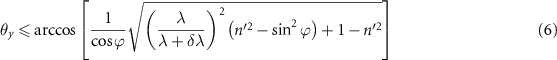
We can further use the Brillouin shift and linewidth values to compare the mechanical properties in the cells of the organoids during morphogenesis. Using the Brillouin images obtained on all nine assemblies for each day of growth ( images with an acquisition time per sampling point of 400 ms), we perform an identification of the regions of the Brillouin images corresponding to the medium surrounding the organoid, its cells or its luminal space, using the array of the shifts of the sample and the Sci-kit Image module [47]. Following this step, we extract the distribution of shift and linewidth values for each of the region corresponding to the cells of the assembly. We perform this study on nine RWPE1 prostatic organoids (including the organoid illustrated in figure 7) over a 14 d of culture. Figures 7(a) and (b) shows the graphs of
  ,
,  in each individual organoid's cells from day 4 to day 15. In this graph, each point corresponds to the average value in one organoid and each error bar is the 95% confidence interval around each point. The same study was conducted on the lumen of the organoids, showing no significant variation with the day of growth of the assembly (see supplementary material).
Figure 8 shows a clear evolution of the linewidth but a stable value for the shift during morphogenesis. This shows that there is an evolution of the mechanical properties during the development of the organoids. To assess the significance of this evolution, we performed a linear regression on all samples and found a significant increase of the linewidth of the cells of the organoid with time (p-value inferior to 10−5) and a negligible evolution of the shift of the cells of the organoid with time (p-value superior to 0.1).
Figure 8. Time evolution of the mechanical properties of the cells of RWPE-1 organoids during their morphogenesis, from day 4 to day 15 after seeding. The figure illustrates (a) the shift and (b) the linewidth values for all nine samples over consecutive measurement days, normalized to daily measures of thermalized ultrapure water. Each data point corresponds respectively to the sample's average (a) shift and (b) linewidth measurement, while the error bars depict the 95% confidence interval on these measurements. We performed linear regressions on the values corresponding to all samples with relation to the day of measure to plot the red lines. The blue area surrounding the linear regression represents the 99% confidence interval for this linear regression.
Download figure:
Standard image High-resolution imageFrom a biophysical perspective it is interesting to underline at the changes in Brillouin linewidth observed here can be attributed to an evolution of the kinematic viscosity, and are not merely the result of a change in refractive index. More specifically, using the expressions for shift and linewidth found in Margueritat et al [15], and assuming that both shift and viscosity of the sample remain constant, the relative changes in Brillouin linewidth Γ and refractive index n are related by:

In average biological scenarios changes in refractive index happen usually on the order of  [48]. A more extreme scenario corresponding to a refractive index evolving between the most contrasted organelles (nucleus 1.355 and lysosome 1.600, see [49]) would lead to
  . In our study, we observe changes of Brillouin linewidth on the order of
  . Therefore, the evolution of linewidth measured here cannot be solely attributed to changes in refractive index, but involves a change in viscosity of the cells during development.
5. Discussion and conclusion
In conclusion, we have evaluated the benefits of using an MMF to couple light to a VIPA spectrometer. The resulting instrument allows improving the collected power in confocal Brillouin scattering measurements by allowing the experimenter to use larger confocal pinhole sizes. Furthermore, the choice of an MMF makes the device both easier to align and more stable in time. One drawback needs however be underlined in our approach: by choosing to use larger pinhole sizes in our confocal arrangement, we increase the amount of collected elastically scattered light. This in turn challenges the filtering of this spectral component. In our approach, we have relied on an absorption cell, an ideal solution that allows for very high extinction ratios with only one requirement on the beam: that the intensity of the light that is to be absorbed by the cell is inferior to its saturation intensity. Practically, absorption cells do not impose a condition on the divergence of the beam, as would étalon used in reflection [50], nor on the beam profile, as would be imposed by the use of destructive interference solutions [51]. Nonetheless, we believe that, through careful dimensioning and alignment, these solutions could still be used to filter out the elastic component of the scattered light collected by an MMF, and thus allows virtually any laser wavelength to be used with an MMF-coupled VIPA spectrometer.
Applying this instrument to the study of the morphogenesis of organoids has allowed to reveal the formation of the hollow structure characterizing acinar or ductal organoids. This observation is however purely morphological and asks for further studies to reveal the biological pathways leading to this cellular organization, as well as their potential effect on the mechanical properties of the cells. Our observation has however shown a remarkable evolution of the Brillouin linewidth inside the cells of the organoid, during its morphogenesis. We can attribute this evolution solely to changes in cell viscosity and consider it unlikely to result from alterations in the solid fraction of the cells.
Finally, we believe the use of an MMF to couple light from a sample to a VIPA spectrometer is a promising configuration for Brillouin scattering experiments, and particularly for the study of biological samples when diffraction-limited spatial resolution is not necessary.
Acknowledgment
The authors thank P Obeid and X Gidrol for the fruitful discussions on the experimental part of this work.
Data availability statement
All data that support the findings of this study are included within the article (and any supplementary files).
Ethical statement
RWPE1 cell line was obtained from ATCC (CRL-3607) and was initially provided by Michigan State University, National Cancer Institute (patent: Webber MM, Rhim JS. Immortalized and malignant human prostatic cell lines. US Patent 5824488 dated 20 October 1998).
H6c7 cell line was obtained from Kerafast compagny (ECA001-FP) (Kerafast, Boston, USA) and was initially provided by the laboratory of Ming-Sound Tsao, MD, FRCPC, University Health Network, Canada.
Appendix A: Characterization of the instrument spatial resolution by knife-edge experiment
The axial resolution of the device was measured using an adapted knife-edge experiment. In order to reduce the amount of elastically scattered light at the interface, we placed a drop of immersion oil on top of a polystyrene plate. The high shift value of polystyrene (around 10 GHz) was high enough that the contrast of our single-stage VIPA spectrometer allowed us to neglect the eventual influence of the elastically scattered light at the interface. We therefore measured the signal intensity of the Brillouin peak of polystyrene around the interface.
Figure A1 shows the intensity of the Brillouin Stokes peak (orange points) and Brillouin anti-Stokes peak (blue points) of polystyrene, taken at different z positions around the interface between the cuvette and the immersion oil. Two Gaussian cumulative distribution functions were then used to fit the points, from which we retrieved two full width at half maximum values which we used to characterize the spatial resolution of the instrument.
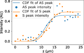
Figure A1. Axial resolution assessed by a knife-edge experiment at the interface between the cuvette and an immersion oil.
Download figure:
Standard image High-resolution imageAppendix B: Geometrical approach of the maximal value for the optimally coupled étendue inside a VIPA étalon
In order to estimate the optimal fully coupled étendue in a VIPA étalon, we will rely on the schematization of the problem proposed in figure B1. Following the parametrization of the figure, we can write:


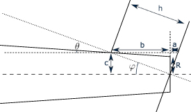
Figure B1. Parametrization of the geometrical approach for the coupling of beams inside a VIPA étalon.
Download figure:
Standard image High-resolution imageFrom there we can directly obtain an expression of the étendue that only depends on the parameters of the VIPA (tilt angle ϕ and thickness h) and on one parameter of the beam, for the following expression, its radius at the plane of focus R:

which in the hypothesis of small angles gives:

This expression is then maximized for ![$R \in [0, h \sin\varphi]$](https://content.cld.iop.org/journals/2515-7647/6/2/025010/revision3/jpphotonad378cieqn121.gif) to find the optimal value for the fully coupled étendue.
to find the optimal value for the fully coupled étendue.
Appendix C: Detailed development of the coupling of étendue inside a VIPA étalon
To assess the coupling of étendue of a beam in a VIPA étalon, we will sum for each element of area of the beam focused on the back focal plane of the VIPA, the solid angle of the beam at this location. Following figure C1(a), this solid angle is essentially defined by a cone of apex angle β from which part part of the angle is 'cut' due to the presence of the front mirror of the VIPA. The difficulty in expressing the coupled étendue lies thus in the expression of the solid angle. Going back to the definition of the solid angle, we can write:

with ν the altitude and φ the azimuth.
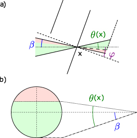
Figure C1. Coupling of a beam focused inside a VIPA étalon. (a) Side representation of a beam of divergence β being focused at a position x on the back focal plane of the VIPA which presents a tilt ϕ. (b) Corresponding coupled portion of the beam shown on the beam profile.
Download figure:
Standard image High-resolution imageWhich for a cone with apex angle 2θ, simplifies to:

Then by using the small angle hypothesis, one can write that the solid angle at any given position is essentially defined as the product of the solid angle of the cone of apex 2β by the ratio of the area of the coupled beam (in green on figure C1) by the total area of the beam. If we first express the green area, we get:

with:


By the change of variable  and applying the identity:
  , we then obtain:

which leads to:

From which we can deduce the formula of the solid angle:

And simplify it in the small angle hypothesis:

which finally allows us to express the coupled étendue:

where R defines the height of the beam along the x axis and, following the conservation of étendue principle, is given as a function of the divergence β of the beam and of the étendue of the fiber:

where  is the diameter of the core of the fiber and NA
 is the aperture of the fiber.
C.1. Expression of the condition of maximal divergence fixed by the maximal curvature allowed
To estimate the angle of maximal divergence allowed in a VIPA spectrometer to allow for considering that the instrument behaves as an SMF device, we will return to the model proposed by Hu et al [42], and particularly equation (7) from his original study, setting θx to 0:

Now to establish condition on the divergence, we need to link the difference in wavelength δλ to the divergence θy of the beam. This leads to:

which after development, writes:
C.2. Detailed development of the distribution of intensity collected
Let us begin by linking the amplitude of the intensity function to the laser's power. This in practice can be done by noticing that the integral of the intensity on the plane of focus of the sample is equal to the laser's power. Therefore:

Then we can establish a relation between the σ parameter, and the full width at half maximum of the function, following:

From there, estimating the collected power comes down to integrating the scattered power on all the observed volume. Assuming that this volume presents a cylindrical symmetry ans is characterized by two Gaussian distribution, along one the axial dimension, with full width at half maximum  and the other the transverse dimension with full width at half maximum
  :
:

which gives:

or after simplification:

Appendix D: Evolution of the mechanical properties of the lumen of organoids
The study performed on the mechanical properties of the cells of the organoids can be completed by the study of the evolution of the lumen of the organoids. Figure D1 presents the result of this study, showing in panel (a), the evolution of the Brillouin shift and in (b) the evolution of Brillouin linewidth, normalized to water. Two comments can be made when compared with figure 8: the shift and linewidth values are lower than for the cells, which shows that the mechanical properties of the lumen of the organoids is different from the one of the cells, and that the evolution of the shift and linewidth is much less pronounced than the one observed in figure 8. With regard to figure 7, we believe this evolution can be imputed to the changes in mechanical properties of the cells of the organoid. The sectioning of our instrument effectively allows part of the scattered signal collected, to originate from the cells of the organoids. We can therefore establish that our study does not conclude on the presence of a change in mechanical properties in the lumen, during morphogenesis of the organoid.
Figure D1. Time evolution of the mechanical properties of the lumen of RWPE-1 organoids during their morphogenesis, from day 4 to day 15 after seeding. The figure illustrates (a) the shift and (b) the linewidth values for all nine samples over consecutive measurement days, normalized to daily measures of thermalized ultrapure water. Each data point corresponds respectively to the sample's average (a) shift and (b) linewidth measurement, while the error bars depict the 95% confidence interval on these measurements. We performed linear regressions on the values corresponding to all samples with relation to the day of measure to plot the red lines. The blue area surrounding the linear regression represents the 99% confidence interval for this linear regression.
Download figure:
Standard image High-resolution image