

Abstract
To mitigate climate change, energy systems must be decarbonised. Human behaviour affects energy systems on residential scales through technology adoption and use, but is often neglected in models for analysing energy systems. We therefore study the optimal planning and operation of a sector-coupled residential energy system driven by economic and environmental interests and user behaviour in terms of desired thermal comfort and clothing. Methodologically, we combine a highly flexible energy system optimisation framework for investment and operational planning, a thermal building representation, a continuous and empirically founded objective for thermal comfort as the sole driver of heating demand and an analytical multi-objective optimisation method in one sector-coupled model. We find that optimal investment in and operation of technology are highly dependent on users' clothing and the desired comfort level. Changing from unadapted to warm clothing in transition and winter season can reduce costs by 25%, carbon emissions by 48%, gas consumption by 84%, heat demand by 20% or necessary PV installations by 28% without lowering thermal comfort. Similar reduction potentials are offered by lowering thermal comfort without changing clothing. We find that heat pumps, rooftop solar PV, batteries and generously sized water tanks are essential technologies that should be adopted regardless of user behaviour, while hydrogen is not. Full decarbonisation would require additional measures like refurbishments or further carbon-free energy sources. We conclude that in striving for decarbonisation and independency of gas, appropriate clothing and sector coupling should be promoted by policy makers and utilised by end-users as very efficient ways of reducing costs, carbon emissions, energy use and gas dependency.
Export citation and abstract BibTeX RIS

Original content from this work may be used under the terms of the Creative Commons Attribution 4.0 licence. Any further distribution of this work must maintain attribution to the author(s) and the title of the work, journal citation and DOI.
1. Introduction
To mitigate the effects of climate change, energy systems must be decarbonised. Countries worldwide have committed to greenhouse gas (GHG) emission reduction targets, for which a transition from fossil fuels to renewable energy sources (RES) is needed [1, 2]. In the EU for instance, RES shares in the electricity sector are growing, but heating and cooling as the largest energy sector is still mostly based on fossil fuels with a share of 75% in 2016 [3]. The EU therefore called for decarbonising buildings with RES-based heating and cooling to achieve their climate targets [3]. More globally, space heating is the largest driver of building energy use in Eurasia and North America with shares of 66% and 48%, while income growth will increase the use of residential heating and cooling in the Global South [4]. [5] found that across four continents, increased electrification of buildings' energy demand and utilisation of RES are necessary to keep global warming below 1.5°C.
This transition towards a RES-based energy system comes with great economic, environmental, technical and social challenges [6–8] and leads to complex decision-making situations, which require tools to adequately inform decision makers. Energy system models (ESMs) have therefore been used for decades to generate insights and support complex decisions in the sector [9]. These models often have a techno-economic focus and obtain a least-cost system design or operation satisfying technical and operational constraints. While challenges are often seen in increasing spatial, temporal and operational detail as well as in treating integrated sectors, uncertainties and high model complexity [9, 10], the human dimension and behavioural aspects remain largely unaddressed [11]. Although often neglected in models, studies have shown that human behaviour significantly affects energy systems at household level through technology choices and user behaviour [12] and at national level through public acceptance [13].
In terms of large-scale infrastructure, [14] found that acceptance for RES-based systems is very high among the German population at the national level, but challenges arise at the local level. [15] showed system and cost effects of social acceptance on transition pathways in the Nordic-Baltic region. In particular, they raised investment costs and constrained capacities for RES generation and transmission lines to account for social acceptance.
On a residential scale, the transition depends on the behaviour and decisions of many individuals. In the residential heating sector, two behavioural aspects greatly contribute to global GHG emissions: decisions to adopt new technologies, i.e. the system design, and the use-patterns, i.e. the operation, of (newly adopted) technologies [12]. In this context, decisions to adopt new technologies are primarily driven by economic factors like household income [16], government support in the form of subsidies [17, 18] and benefits in terms of energy-bill savings [19, 20]. However, environmental concerns also positively influence adoption [21–23]. External factors like the peer effect influence adoption decisions [24], but lie beyond the energy systems themselves.
While the presence and choice of technologies play a key role, the associated user behaviour also largely determines the final energy demand [25, 26], driven by monetary and non-monetary incentives [27]. For instance, German households were able to reduce their gas consumption substantially by changing heating behaviour in 2022 [28]. Such demand reductions can be achieved by lowering the set temperature, which is a key driver for heating energy demand [29, 30]. However, temperature reductions might have adverse effects on occupants' thermal comfort, which can be counteracted by increased clothing or physical activity [31]. [32] showed that flexible clothing enables energy savings without lowering thermal comfort. [33] found that clothing and metabolic rate have even higher impact on energy consumption and residents' comfort than building parameters. [34] used real-time clothing information in an office building's heating and cooling operation to reduce power consumption while enhancing comfort. Although this connection between comfort, clothing, indoor temperature and energy savings matches everyday experience, it needs further quantitative analysis to inform decision making. Energy savings are often means to achieving economic or environmental targets. Their relation depends on the specific context and energy system considered and needs quantification. Furthermore, while the connection is well-established on the operational level, it remains unclear how costs or emissions can be saved through effects on system design or investment decisions.
To summarise, through the adoption and use of technologies, the residential energy transition is driven by competing interests related to costs, GHG emissions and comfort. Multi-objective optimisations have been used by many studies to consider multiple such interests in energy system models [35, 36]. Analyses with multiple objectives can provide better decision support than single solutions obtained by either ignoring some interests completely or making a priori assumptions about people's preferences [37]. First, ignoring existing interests leads to inefficient or socially infeasible solutions. Second, single solutions provide incomplete information about what energy systems are possible and leave the full scope for and consequences of decision making undiscovered [38, 39]. Finally, determining preferences without knowledge about alternatives, their consequences and trade-offs comes with great uncertainties and inaccuracies [40].
The existing literature on multi-objective analysis of residential energy systems falls into at least one of the following categories. In the first category, studies optimised building energy systems for multiple objectives, but neglected thermal comfort [41–46]. In the second category, studies used a thermal comfort objective for a multi-objective optimisation, but did not optimise the design and operation of a residential energy system. Instead, they studied the building design [47–50], retrofitting [51–53], or non-residential objects [54–56]. In this group, neglecting the different energy supply technologies often lead to the use of objectives related to energy consumption, efficiency or cost [48–52, 54, 56, 57] but not GHG emissions. In the third category, studies used a comfort objective but did not consider an empirically-founded, continuous comfort metric. Instead, they mostly used an asymmetric step function with a discomfort value of one below and a value of zero above a certain temperature threshold [49, 51, 52, 54, 55, 58] which lead to static temperature profiles, while others employed metrics without empirical foundation like one-directional deviation [58]. In a fourth group, existing studies [41, 44, 46–48, 50, 56, 57] used building-level simulation models like EnergyPlus 1 and coupled these with heuristic algorithms, for example the Non-dominated Sorting Genetic algorithm (NSGA) II [59], to make simulation results iteratively converge towards a Pareto front. If the building is described in a simulation model that itself does not optimise, then the coupling with a heuristic is necessary to approximate Pareto-optimal solutions by carrying out a large number of simulations. If, in contrast, the building is integrated in an optimising model, then analytical multi-objective optimisation methods like the weighted sum or augmented epsilon-constraint method can be used to obtain a guaranteed Pareto-optimal solution with each individual model solve.
As a main novelty, this work integrates the continuous and empirically-founded metric Predicted Percentage Dissatisfied (PPD) [31] for thermal comfort in the multi-objective investment and operational optimisation of a sector-coupled residential building in an energy system model. In particular, we consider GHG emissions, costs and thermal comfort as three objectives in a multi-objective optimisation and compare different levels of comfort and three clothing scenarios to analyse and quantify impacts of human behaviour on the residential energy transition under the conflicting targets. A joint optimisation of energy system operation and design allows user behaviour to impact not only scheduling but also investment decisions. By integrating a thermal building representation into an optimising energy system model instead of using a building simulation, we can utilise the analytical augmented epsilon-constraint method [60] for the multi-objective optimisation instead of relying on heuristic approaches. In this work, we use an exemplary building in Germany to derive quantitative results. The methodology can be transferred to any other building or region by adapting model parameters and we expect results to be transferable to buildings/regions with similar parameters.
More specifically, we aim at answering the following questions:
- How does user behaviour affect optimal choices for technology adoption and operation in residential power and heat systems in light of the conflicting objectives of costs, carbon emissions and thermal comfort?
- To what extent can user behaviour reduce costs and carbon emissions as well as energy and gas consumption in residential power and heat systems?
- What recommendations can be derived for end-users, policy makers and energy system modellers regarding user behaviour in residential energy systems?
The remainder is structured as follows. Section 2 outlines the methodology, section 3 presents and discusses results and section 4 concludes.
2. Methodology
The methodology has three main pillars, (i) an energy system model of a building equipped with an endogenous measure of indoor temperature, (ii) an objective function mapping indoor temperature to an empirical measure for occupants' thermal comfort and (iii) a multi-objective optimisation method generating Pareto-optimal solutions for the conflicting objectives of costs, CO2 emissions and thermal comfort.
2.1. Building model
The representation of a typical unrefurbished building in Germany is based on an existing model [61], which is implemented in the energy system optimisation framework Backbone [62]. Energy system models in Backbone are composed of grids grouping nodes as well as units converting energy between nodes and across grids. Backbone is highly flexible in terms of systems it can represent, for example sector-coupled individual buildings, municipal systems or multi-national networks [37, 63, 64], and openly available at https://gitlab.vtt.fi/backbone/backbone.
In the building model, which is shown in figure 1, a fuel grid allows for procurement of gas and electricity at retail price levels from 2019 [65, 66] being 62 €/MWh for gas and 305 €/MWh for electricity. Furthermore, the CO2 emission intensities of electricity and gas are 408 kg/MWhel [67] and 182 kg/MWhth, respectively. The only source of carbon-free energy is rooftop PV, whose installation potential is limited according to 80% of the building footprint.
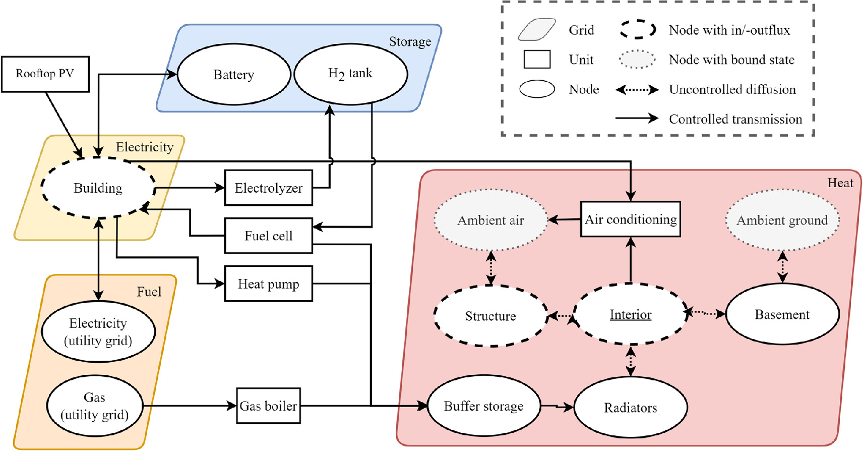
Figure 1. Schematic representation of the sector-coupled residential building energy system model. There are no pre-installed capacities and investments into all units and storage capacities are possible. Nodes with bound state have a fixed temperature that the model cannot influence. Influx to nodes are caused by solar gains while outflux represents power demand. The temperature of the underlined 'Interior' node is used to model occupants' thermal comfort as described in section 2.2.
Download figure:
Standard image High-resolution imageThe building itself is defined by a set of connected nodes in the heat grid as depicted in figure 1. The building's structure, basement and interior are each represented as a node and parameterised according to table 1. Since the effective heat transmission is implemented in W/K, U-values are multiplied with the respective area. For the structure node, a weighted average of the roofs' (1.0 W/(m2K)), walls' (1.4 W/(m2K)) and windows' (2.7 W/(m2K)) U-values has been calculated. To do so, a roof-to-wall ratio of 73% and a window-to-wall ratio of 20% was used. By considering thermal inertia, nodal energy content is endogenously translated into the components' temperature. For the temperature of the ambient ground and air, fixed time-series from a German weather station [68, 69] are used. Unintended energy diffusion occurs between the interior, basement and ambient ground as well as the interior, structure, and ambient air nodes based on U-values and temperature differences. The temperature of the building's nodes can be controlled intentionally by the heating and cooling units' operation via the buffer storage and radiators within certain bounds that are explained in section 2.2. Therefore, heat demand is determined implicitly depending on the desired indoor temperature, temperature differences between the building's and the ambient nodes, U-values and respective areas of structural components.
Table 1. U-values, areas and heat capacities of building components used to parameterise the model.
| Building components | U-value (W/(m2K)) | Area (m2) | Heat capacity (Wh/(m2K)) |
|---|---|---|---|
| Structure | 1.38 | 276.00 | 48.61 |
| Basement | 1.24 | 87.20 | 31.11 |
| Interior | n.a. | 147.10 | 2.78 |
| Source | [70] | [70] | [71] |
To meet this heat demand, the model can invest in a heat pump or a gas boiler or utilise waste heat from a fuel cell according to the costs presented in table A1. Via a buffer storage and radiators, this heat is ultimately transmitted to the interior. Furthermore, an electrolyser allows for generating hydrogen, which can be stored in a hydrogen tank and a battery allows for electricity storage. The techno-economic parameters of these units are taken from [72]. An air conditioning (AC) unit is available for cooling. Additionally, an electricity demand must be met that accumulates to 5.5 MWh annually [73].
To summarise the decision space, this model optimises the invested capacities of all appliances (rooftop PV, gas boiler, heat pump, air conditioning, fuel cell, electrolyser, H2 tank and battery) and for each time step their operation and the use of gas and electricity from the utility grid. Additionally, the energy content of the storage nodes (H2 tank, battery, buffer storage), the building nodes (basement, interior, structure) and the radiator node are decision variables that can be controlled by the operation of units.
To keep the computation of hundreds of solutions tractable, time-series of ambient air and ground temperature, solar radiation, electricity demand and coefficient of performance (COP) of the heat pump [74] are aggregated from one year in hourly resolution to three typical periods, each one week long with the same resolution. This is achieved by using the Time Series Aggregation Module (TSAM) [75] on all time series of our model. It is used with the settings of a period length of 168 hours, period number of three and cluster method 'hierarchical', which yielded the lowest information loss. Although the resulting typical periods do not exactly depict a specific period of the original data, they can be thought of as representing a winter, transition and summer season. In more detail, the aggregated time-series represent weeks of low (winter, 11 weeks), medium (spring and fall, 16 weeks) and high (summer, 25 weeks) temperatures.
2.2. Thermal comfort
Endogenising indoor air temperature as the energy content of the 'Interior' node allows for assessing the occupants' thermal comfort by using the Predicted Percentage Dissatisfied (PPD). The PPD [31] is an empirically-founded metric prevalent in the scientific literature [50, 55, 76] and national standards [77, 78]. It represents the share of people dissatisfied with the climatic indoor conditions based on the temperature, relative humidity and air speed as well as a person's metabolic rate and clothing insulation.
When fixing the values of all inputs except the temperature T, the PPD can be approximated as a linear function of the deviation from a set temperature, i.e. using only three parameters mset, Tset and PPDoffset:

In this study, we choose an air speed of 0.1 m/s, which is in line with no ventilation, and a relative humidity of 50%, which is in the range proposed in the standard [77] and also mentioned to have a rather small impact on thermal comfort in moderate climates and even found to be negligible by [76]. By definition of the PPD [31], we fix the offset PPDoffset = 5%. Furthermore, we use time series for the occupants' metabolic rate and clothing level. We assume a metabolic rate of 1.0 met (=58 W/m2) (seated, awake, writing or reading) for daytime from 7 h to 23 h and 0.7 met (lying, sleeping) for nighttime from 23 h until 7 h to reflect typical temporal variations in activity level [76]. To depict a range of possible clothing behaviour, we study three different clothing level scenarios. The daytime clothing ranges from typical summer indoor clothing with 0.5 clo over typical winter indoor clothing with 1.0 clo (=0.155 m2K/W) up to warm clothing with 1.5 clo. Nighttime clothing [76] ranges from short pyjamas and partial coverage with a bed sheet (1.43 clo) up to long pyjamas and full coverage with a quilt (4.56 clo). For more details on clothing and metabolic units the reader is referred to [77–79].
We distinguish the clothing between three seasons (winter, transition, summer) based on the weather data sampling and construct a light, medium and warm clothing scenario. The clothing levels and set temperatures per scenario, season and daytime are shown in table 2.
Table 2. Clothing insulation as well as fitted values for Tset, mset,  and
and  per scenario, season and time of day.
| Scenario | Season | Clothing (clo) | Tset(°C) | mset(%/°C) |
 (°C) (°C) |
 (°C) (°C) | |||||
|---|---|---|---|---|---|---|---|---|---|---|---|
| Day | Night | Day | Night | Day | Night | Day | Night | Day | Night | ||
| Winter | 0.50 | 2.40 | 26.00 | 23.00 | 6.27 | 4.08 | 23.00 | 18.50 | 29.00 | 27.50 | |
| Light | Transition | 0.50 | 1.80 | 26.00 | 24.75 | 6.27 | 4.98 | 23.00 | 21.00 | 29.00 | 28.50 |
| Summer | 0.50 | 1.43 | 26.00 | 26.00 | 6.27 | 5.73 | 23.00 | 22.75 | 29.00 | 29.25 | |
| Winter | 1.00 | 4.34 | 23.25 | 17.00 | 4.52 | 2.65 | 19.25 | 10.00 | 27.25 | 24.00 | |
| Medium | Transition | 0.75 | 2.62 | 24.75 | 22.25 | 4.87 | 3.82 | 21.50 | 17.50 | 28.00 | 27.00 |
| Summer | 0.50 | 1.65 | 26.00 | 25.25 | 6.27 | 5.18 | 23.00 | 21.75 | 29.00 | 28.75 | |
| Winter | 1.50 | 4.56 | 20.50 | 16.50 | 3.57 | 2.54 | 15.50 | 9.25 | 25.50 | 23.75 | |
| Warm | Transition | 1.00 | 2.88 | 23.25 | 21.50 | 4.52 | 3.51 | 19.25 | 16.50 | 27.25 | 26.50 |
| Summer | 0.50 | 2.15 | 26.00 | 23.75 | 6.27 | 4.50 | 23.00 | 19.50 | 29.00 | 29.00 | |
For each clothing level and metabolic rate, we fit the parameters mset and Tset to PPD data obtained with the CBE Thermal Comfort Tool [79]. In figure 2, the fitted functions for PPD(T) are displayed together with the exact PPD values for selected clothing levels and metabolic rates. This results in a time series for each parameter and scenario, which we use as input data for the model. Additionally, upper and lower bounds  for the indoor temperature are enforced so that the PPD cannot exceed 30%, i.e.
  . This corresponds to allowed deviations between 3 °C and 7.25 °C from the set temperature. The resulting parameter values are also shown in table 2.
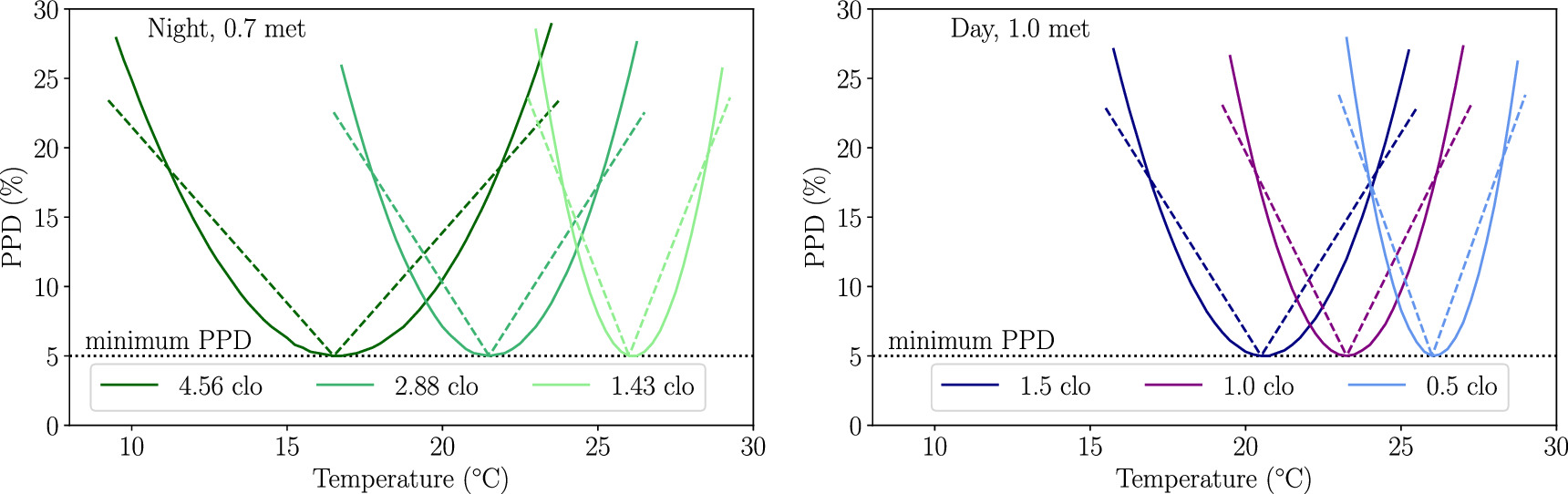
Figure 2. Exact PPD values (solid lines) and fitted functions (dashed lines) used in linear energy system model for nighttime with 0.7 met (left) and daytime with a metabolic rate of 1.0 met (right) and different clothing levels.
Download figure:
Standard image High-resolution image2.3. Multi-objective optimisation
The simultaneous optimisation of multiple real-valued objective functions is called multi-objective optimisation. A solution to such a problem is called Pareto-optimal if one objective can only be improved when deteriorating another. The set of all Pareto-optimal solutions is called Pareto front. For an overview and introduction to the theory of multi-objective optimisation, see e.g. [80]. As the building representation and comfort metric are implemented and parameterised in an optimising energy system model, objective functions can be included directly in the model without necessity for any coupling to heuristic algorithms or other models.
Building upon an implementation [37] of the augmented epsilon-constraint method (AUGMECON) in Backbone, we optimise the model for three objectives simultaneously. The objectives to be minimised are system costs, carbon emissions and thermal discomfort. System costs

include costs for variable and fixed operation and maintenance ( and cFOM), fuel
  and annualised investments cinvest. Carbon emissions

arise from the use of grid electricity  and natural gas
  . Occupants' average thermal discomfort

is based on the PPD metric. Each time step t is weighted with wt ≥ 1 to account for the longer period it represents.
Applying AUGMECON [60], the multi-objective optimisation problem

is reformulated to


by introducing a small scalar c ≈ 10−6...10−3, two non-negative slack variables s1,2 and two constants k1,2 reflecting the typical order of magnitude of the objectives femission and fdiscomfort, respectively. The implementation of the PPD as well as the comfort and other objective functions in Backbone is openly available from https://gitlab.vtt.fi/backbone/backbone.
For each choice of upper bounds εemission and εdiscomfort, the solution to this reformulated problem is a Pareto-optimal solution to the original multi-objective optimisation problem (5). Solving the reformulated problem multiple times for varying upper bounds yields a representative subset of the whole Pareto front. Single-objective optimisations of (2), (3) and (4) give estimates of the Pareto front boundaries and hence the region ![$\left[{\varepsilon }_{\min }^{\mathrm{emission}},{\varepsilon }_{\max }^{\mathrm{emission}}\right]\times \left[{\varepsilon }_{\min }^{\mathrm{discomfort}},{\varepsilon }_{\max }^{\mathrm{discomfort}}\right]\subset {{\mathbb{R}}}^{2}$](https://content.cld.iop.org/journals/2515-7620/5/11/115009/revision2/ercad0990ieqn11.gif) that should be covered by the two upper bounds.
that should be covered by the two upper bounds.
To save modellers' and computational time, the steps of (i) single-objective optimisations, (ii) determination of upper bounds and (iii) multi-objective optimisations with AUGMECON are automated and parallelised using a python script that is openly available from https://gitlab.ruhr-uni-bochum.de/ee/backbone-tools. While the three steps have to be carried out subsequently, parallelisation is possible within each step. In the third and most computationally heavy step, where thousands of optimisation problems are solved, this parallelisation is particularly beneficial for reducing computational time.
Since the discomfort objective contains an absolute value, a reformulation is necessary for the implementation in a linear ESM. Generally, to linearise the absolute value ∣x∣ of a variable with upper bound  , introduce two non-negative variables x+, x− ≥ 0 and a binary variable b ∈ {0, 1} such that


Then, the linear expression x+ + x− takes the absolute value of x. This can be shown by considering the two cases b = 0 and b = 1 and noting that x+ = x and x− = 0 if x > 0 and x+ = 0 and x− = x if x < 0. To implement the comfort objective function in Backbone, we used the above approach with  for each time step t and a high enough value for
  to not impose any additional constraints on the model.
2.4. Analysing and visualising the solution space
For the building energy system model, about 500 Pareto-optimal solutions are determined per clothing level, each of which is an hourly investment and operational optimisation. To generate insights from the resulting amount of data, we choose to fix some of the objectives (cost, emission, discomfort) at a certain level and analyse changes along the remaining degrees of freedom. Some of the quantitative results presented in section 3, e.g. saving potentials for costs, emissions, energy or gas, depend on this choice of objective values and are therefore somewhat illustrative. However, we aim at indicating and visualising how the results change under varying choices. The complete results are available and can be explored interactively at https://apps.ee.ruhr-uni-bochum.de/Comfort.
To study the impact of human behaviour related to thermal comfort, we analyse two ways of influence separately. First, we investigate the medium clothing scenario and compare different comfort levels, and second, we keep a constant comfort level and compare different clothing scenarios. For both analyses, we show results in three ways: the whole Pareto front(s) in 3D solution space, subsets of the Pareto front(s) in 2D for which either discomfort or clothing scenario is kept constant (referred to as slices) as well as the heat and power generation per technology along those slices. The quantitative results of costs, emissions and energy consumption always refer to the modelled period of one year. Investment costs are annualised and the PPD results are time-averaged. Additionally, we show the invested generation and storage capacities as well as full load hours for three such slices and analyse what deviations from the optimal temperature lead to certain levels of discomfort.
3. Results and discussion
The model results are presented by analysing varying levels of thermal discomfort and clothing levels as well as a brief explanation of how the average change in PPD is distributed over the model horizon and how that affects system design and operation.
3.1. Impact of varying levels of thermal comfort
The shape of the whole Pareto front for medium clothing as shown in figure 3 indicates that a strong trade-off exists between costs and emissions, whereas the trade-offs between costs and comfort as well as comfort and emissions are weaker. To inspect the results in more detail, we analyse slices at fixed discomfort levels of 5.3%, 8.9% and 12.8% average PPD, which are highlighted in figure 3 in darkening shades of grey. As a general pattern, the slices are shifted to lower emissions and lower costs for higher discomfort. In particular, the boundaries of the slices depend on the comfort level. The lowest possible costs and emissions exhibit differences of 600 € and 0.7 t, respectively, between the outermost slices. Lowest possible emissions are driven by the limited available carbon-free energy from rooftop PV investments and the emission factor of grid electricity, which is an exogenous model parameter that is constant in time. By using temporally resolved emission factors, further decarbonisation could be achieved by the model. The highest Pareto-optimal costs and emissions exhibit differences of 2900 € and 1.3 t, respectively. The trade-off between costs and emissions is rather independent of the comfort level, as indicated by the slope of the slices. For the slice with 5.3% PPD, the steeper region from 2.9 t to 4.8 t has an almost constant slope with average CO2 abatement cost of 570 €/t. The flatter region above 4.8 t has a slope of 90 €/t, while the very low emissions below 2.9 t come at marginal CO2 abatement costs of 7130 €/t. The slices with higher discomfort exhibit regions with similar steepness, but the regions themselves are shifted towards lower emissions and costs. The marginal CO2 abatement costs indicate, what (additional) carbon prices would be necessary as a financial incentive for purely cost-minimising actors to achieve the respective emission reduction.
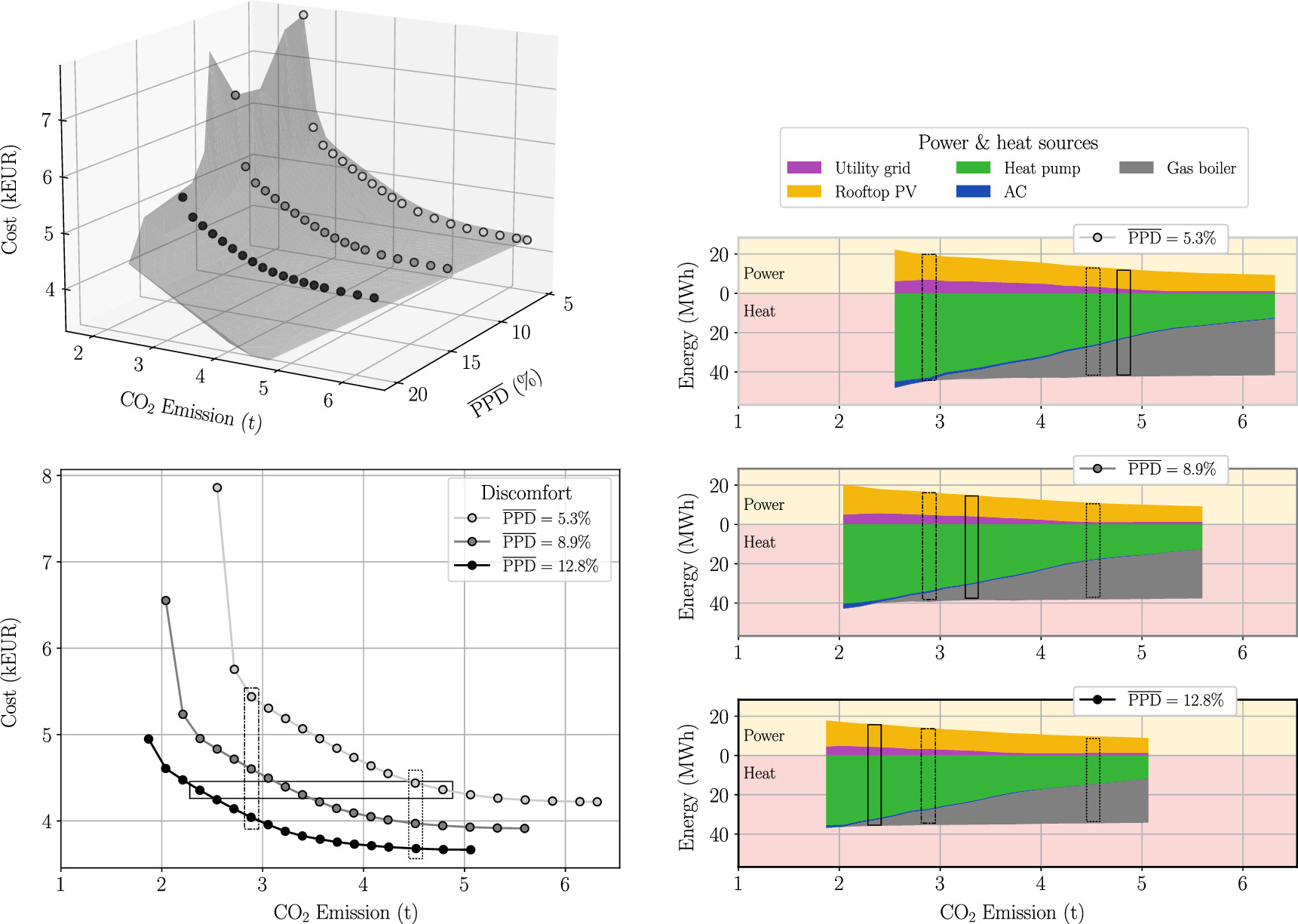
Figure 3. Pareto-optimal solutions for the medium clothing scenario. The left side shows the Pareto front in 3D objective space (top) and three slices with fixed levels of discomfort projected in 2D (bottom). The right side shows power and heat generation per technology for the three slices as area charts. Power is indicated above the 0 MWh-line in the yellow shaded area, whereas heat is shown in the red shaded area below the 0 MWh-line. Black boxes highlight solutions of constant costs or emissions for further analysis.
Download figure:
Standard image High-resolution imageThe three slices allow for analysing the potential cost and emission savings achievable by reducing comfort, as indicated by the black boxes in figure 3. For fixed emissions of about 2.9 t (dash-dotted boxes), costs decrease from 5400 € to 4600 € and 4000 € when increasing discomfort from 5.3% PPD to 8.9% PPD and 12.8% PPD, respectively. At this emission level, the relative cost saving potential through decreasing comfort by 7.5% points amounts to 26%. At higher emissions of 4.5 t (dotted boxes), the absolute cost-saving potential is only half as high. Allowing for the first discomfort reduction of 3.6% points reduces system cost by roughly 400 €. The cost saving reduces to 300 € for the next 3.9% point difference in PPD. Generally, we observe a typical trend of diminishing marginal utility, i.e. increases in discomfort have the largest impact close to the lowest possible PPD and lowest possible emissions and diminish with further increases in discomfort or emissions.
In terms of energy, increased discomfort reduces the overall power and heat generation. At emissions of 4.5 t, for instance, the generated heat reduces from over 42 MWh to 34 MWh, i.e. by 19% for a 7.5% points higher PPD. Furthermore, the use of heat pumps and grid electricity decreases, being replaced by increased utilisation of the gas boiler. Since increased discomfort allows for larger or longer deviations from the set temperature, the required heat generation decreases for increased discomfort. If allowed emissions are fixed, the model saves costs by using a higher share of gas for heating thus decreasing the more costly use of heat pumps that would also require more grid electricity.
Viewed from the other objective direction, when maintaining a fixed level of system cost at around 4400 € (solid boxes), emissions drop from 4.8 t to 3.2 t when allowing 8.9% PPD instead of 5.3% PPD. For the subsequent increase in discomfort to 12.8% PPD, emissions decrease further to 2.4 t. This roughly translates to an emission reduction potential of 6.9% of per % point increase in discomfort. Here, the relative emission saving potential amounts to 50% through accepting an increase of 7.5% points in discomfort without increasing costs.
In terms of energy, decarbonisation is achieved by increased utilisation of heat pumps that replace gas boilers for heating. This leads to increased power demand which is met by increased solar PV generation as well as imports from the utility grid. This also implies a shift in imported energy from gas to power resulting from the price and efficiency assumptions that make gas heating cheaper but more carbon-intensive as compared to a heat pump combined with grid electricity. This trend additionally reveals a gas saving potential of 16 MWh heat energy between the outermost slices without any cost increase. This is partially compensated by increased use of grid electricity, which increases by 2 MWh difference. Since the current share of gas in the German power mix is around 15%, the increase in utilised grid electricity hardly reduces the effective gas saving potential.
Furthermore, the use of air conditioning increases with decreasing emissions. Hence, increased cooling in summer is a more emission-efficient way of achieving the same average discomfort level. The fact that this trend coincides with higher PV generation and battery investments (see figure 6) can possibly be explained by an increased self-consumption of the emission-free PV power in summer replacing grid electricity in winter. This is due to the higher natural correlation between electricity demand for cooling and PV generation. The finding can also be explained by the variations in clothing level and its effect on the temporal distribution of discomfort over the seasons.
Generally, it is challenging to compare our quantitative findings with other studies. First, the studied objects are often not comparable. Second, different studies employ different objective functions in terms of both cost and comfort. Third, many studies do not explicitly model design choices between different energy generation technologies. While this again emphasises the novelty of our work as described in the introduction, it means that a direct comparison of absolute saving potentials or the explicit design and operation of the energy system is impossible. However, by comparing the slope of Pareto front slices, comparisons can be made regarding the trade-offs between comfort and costs as well as comfort and overall energy consumption.
The trade-off between cost and comfort in this work can be approximated to a 3.5% decrease in annual cost per % point increase in discomfort, which is in line with other studies. [52] found a trade-off between cost and the total percentage of discomfort hours as approximately 3.3% cost reduction per % point increase in discomfort. Similarly, [57], where the comfort objective is to minimise the highest value of PPD, the trade-off with operation costs can be approximated by a 2.6% cost reduction per % point increase in comfort.
Regarding the trade-off between energy use and comfort, we find a value of 2.5% decrease in energy use per % point increase in discomfort in this work. Although [52] quantify specific energy intensity per square metre, they found a trade-off of similar magnitude with 1.75% decrease in energy use per % point increase in their discomfort metric. The same energy use metric is utilised by [49], who employed a comfort objective of 'discomfort time ratio' and found a trade-off of 3.2% decrease in energy use per % point increase in the discomfort metric.
3.2. Translation of discomfort to temperature deviations
Increased discomfort corresponds to a greater deviation of the realised interior temperature T from the set temperature Tset. For example, during daytime (1.0 met) in the transition season and the medium clothing level of 0.75 clo, the slope of the linear fit is mset = 4.87 %/°C. Therefore, PPD differences of 3.6% points and 7.5% points correspond to an additional average deviation ∣Tset − T∣ of 0.7 °C and 1.5 °C, respectively. Hence, the respective changes in average PPD as discussed in section 3.1 could result from exactly this additional but small and constant deviation in each time step and from temperatures above or below the set temperature. The results as shown in figure 4, however, reveal most deviations to be in the eleven winter weeks, i.e. rare and heterogeneous, below the set temperature, i.e. asymmetric, and larger than a constant deviation would necessitate, e.g. from 3 °C to 7 °C for a PPD of 8.9%. More specifically, hours accumulate around the highest possible deviations of −7 °C during night and −4 °C during daytime in winter.
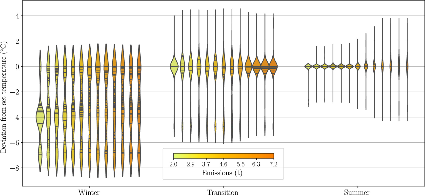
Figure 4. Deviations from the set temperature per emission level (indicated by colour) and season for an average PPD of 8.9%. With decreasing emissions, deviations accumulate in summer and transition season at 0 °C indicating lower discomfort in these seasons. This allows for larger deviations in winter as shown by the accumulation at around -4 °C and -7 °C. Thus, the overall discomfort is held constant, but shifted from summer to winter to save emissions while increasing costs. Note that the solutions shown here correspond to the central slice in figure 3.
Download figure:
Standard image High-resolution imageThis trend towards negative deviations of high magnitude in winter is caused by two factors. The first is the geographical region, i.e. the fact that ambient temperatures are mostly lower than the set temperatures with the largest differences in winter causing higher heat transmission losses towards the ambient air and ground. The second factor is the PPD's characteristic that its slope mset decreases with higher clothing levels, i.e. the fact that in winter, when warmer clothing is used, the same temperature deviation translates into a smaller PPD difference than it would in summer with lighter clothing (compare figure 2 and table 2). Hence, few strong temperature deviations in winter require less heating energy than many small deviations in other seasons and can therefore reduce emissions.
However, reducing emissions in this way reduces overall comfort. To reduce emissions while keeping overall discomfort constant, figure 4 reveals that temperature deviations shift from summer to transition and finally to winter. This is achieved by making increased use of the solar energy source for cooling and heating when it is most abundant. While positive temperature deviations might appear cost-inducing at first, this is not the case in warmer seasons, where outdoor temperatures above the set temperatures would require cooling.
While figure 4 only shows results for one level of discomfort, we can say that deviations are reduced for decreasing PPD levels, which leads to accumulations shifting towards 0 °C.
3.3. Impact of varying clothing level
Instead of altering comfort levels, occupants may change their clothing to affect the perceived thermal comfort. To illustrate the effects of clothing, Pareto-optimal solutions of three scenarios with light, medium and warm overall clothing (see table 2) are presented in figure 5 as a blue, grey and red surface, respectively. Each scenario consists of a time series of clothing levels, which can differ by season (summer, transition, winter) and time of day (day, night). The light clothing scenario is almost unadapted to the seasons. In the medium and warm clothing scenarios, the clothing gets increasingly warmer in transition and winter while remaining almost unchanged in summer. In that sense, the medium and warm clothing scenarios can be considered more 'appropriate'.

Figure 5. Pareto-optimal solutions for the different clothing scenarios. The left side shows the Pareto fronts for light and medium clothing (top left) and medium and warm clothing (top right) in 3D objective space and three slices with a fixed level of discomfort (PPD = 5.3%) projected in 2D (bottom). The right side shows power and heat generation per technology for the three slices. Electricity is indicated above the 0 MWh-line in the yellow shaded area, whereas heat is shown in the red shaded area below the 0 MWh-line. Black boxes highlight solutions of constant costs or emissions for further analysis. Note that the medium clothing slice is the same as the lowest discomfort slice in figure 3.
Download figure:
Standard image High-resolution imageThe relative positions of the three Pareto fronts indicate that lighter, unadapted clothing (blue surface) correlates with higher costs and emissions while warmer clothing (red surface) in winter and transition season correlates with lower costs and emissions. By considering slices at a PPD of 5.3%, which are highlighted as dots, we analyse the cost, emission, energy and gas savings achievable through more appropriate clothing without comfort losses. The slices show a general shift towards lower emissions and costs for increasing clothing level. The Pareto front boundaries vary significantly between the clothing levels. The lowest possible costs differ by 700 € or a factor of 6/7 between the light and warm clothing. The lowest possible emissions change by 1 t or a factor of 2/3, indicating that certain decarbonisation or cost targets can only be achieved with adapted clothing. In particular, the previously compared levels of 2.9 t and 4400 € (see section 3.1) cannot be achieved with light clothing. The level of the CO2 abatement costs is almost independent of the clothing scenario, but a shift of the more or less steep regions can be observed.
At emissions of 4.5 t (dashed black boxes), changing from the light to the medium clothing scenario, i.e. to warmer clothing in winter and transition season, reduces cost by roughly 860 €, whereas changing from medium to warm clothing reduces cost only by 400 €. These absolute differences are almost constant for emissions below 4.5 t (and above 3.5 t) and decrease for higher emissions. With warmer clothing, cooler indoor temperatures result in the same comfort, hence the heat and power generation decrease. At 4.5 t, for instance, heat generation reduces from 45 MWh to 37 MWh, i.e. by 18% between the light and warm clothing. At unchanged emissions, this induces the cost saving potential, as less heat generation has to be shifted from the cheaper but more carbon-intensive gas boiler towards the more costly but less carbon-intensive heat pump.
In the other objective direction, solutions of equal costs reveal emission savings for higher clothing levels. For costs of roughly 4700 € (solid black boxes), emissions are reduced from 5.9 t to 3.9 t for changing from the light to the medium clothing scenario, and finally to 3.1 t for the warm clothing scenario. Thus, changing from lighter, unadapted to warmer, more appropriate clothing in transition and winter can reduce total emissions by almost 48%. In terms of energy generation, this decarbonisation is achieved by reducing the use of gas boilers and increasing the use of heat pumps together with solar PV and grid electricity. This indicates that at this cost level, 21 MWh heat energy in the form of gas can be saved by adapted clothing without increased discomfort or increased cost. This gas saving is to a small extent compensated by increased consumption of grid electricity that partially relies on gas itself, but mostly constitutes a genuine gas saving.
As with the behavioural impacts in terms of different comfort levels, comparing the quantitative findings regarding the impact of clothing levels to other literature is challenging due to differences in modelling approach and scope. In terms of trade-offs between clothing and energy consumption, [34] stated that a clothing level adaptation of 0.1 clo can lead to energy savings of 16% in summer and 13.7% in winter. In our work, the seasonally weighted difference between the light and warm clothing scenario is 0.6 clo, which translates to a significantly lower value of 3% per 0.1 clo. This difference could be explained by many factors. First, our quantitative findings in terms of saving potentials due to behavioural changes in terms of clothing vary significantly between and within the Pareto front slices, i.e. they depend on the choice of comfort, cost and emission levels. Second, in our multi-objective optimisation model, energy savings are not an objective, but one of many possibilities to achieving the more fundamental targets of saving costs or emissions, thus potentially leaving energy saving options undiscovered. Third, we implement clothing changes for different metabolic rates during day and night time, which impacts its effect on the set temperature, but might be a more realistic assumption.
3.4. Energy system design and operation
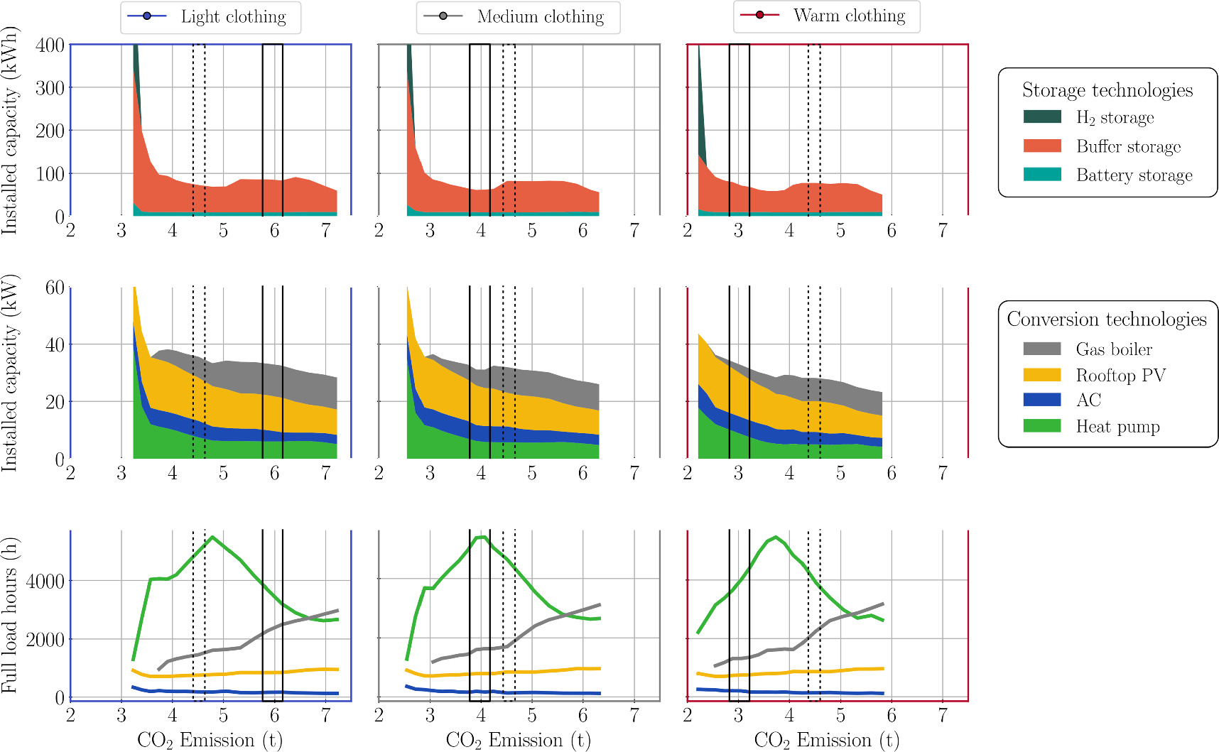
In terms of invested storage and conversion capacities as well as the latter's full load hours (see figure 6), we make four observations. First, the model achieves decarbonisation through substituting the gas boiler investments by investments in a heat pump across all scenarios. Generally, the results are dominated by bivalent systems with significant capacities of both heat pump and gas boiler. Low full load hours indicate that the gas boiler tends to serve peak loads, in particular for lower emissions. Above 4.8 t for light, 4.0 t for medium and 3.7 t for warm clothing, decarbonisation is achieved by increased utilisation of almost constant heat pump capacities, while reducing the utilisation of almost constant gas boiler capacities. This indicates that a certain amount of decarbonisation can be achieved by operational changes. Deeper decarbonisation below aforementioned emission levels requires changes in the system design in the form of over-proportional heat pump investments together with a phase-out of the gas boiler. This is indicated by the strong decrease in heat pump full load hours, in particular for very low emissions and low clothing. Furthermore, the decarbonisation by changed clothing levels at a constant cost level of 4700 € manifests in differently sized appliances as indicated by table 3. Most significantly, the optimal gas boiler capacity reduces by 72% from light to warm clothing. Not each combination of installed gas boiler and heat pump capacities might be widely used or feasible in reality. However, constraining the model to certain discrete capacities limits the solutions obtained and hence does not generate more, but only less insights.
Figure 6. Installed capacities of energy storage (top) and conversion (center) technologies as well as the latter's full load hours (bottom) for the light (left), medium (center) and warm (right) clothing scenarios and different CO2 emissions with a fixed PPD of 5.3%. The solutions shown here correspond to the slices in figure 5 with analogous highlighting of solutions with equal cost (solid black boxes) and equal emissions (dashed black boxes). Generally, buffer storage capacities are much higher than battery capacities. Heat pump and PV investments increase with decreasing emissions, thereby substituting the gas boiler investments. The installed capacities for AC show a smaller increase. With decreasing emissions, the gas boiler is increasingly used for peak demands, while the utilisation of heat pump capacities peaks for medium emissions.
Download figure:
Standard image High-resolution image
Table 3. Detailed results of system design under varying clothing levels at fixed emissions (top half) and fixed costs (bottom half).
| Clothing level | Cost (k€) | Emission (t) | Battery (kWh) | Buffer tank (kWh) | Heat pump (kW) | AC (kW) | PV (kW) | Gas boiler (kW) |
|---|---|---|---|---|---|---|---|---|
| Light | 5.3 | 4.5 | 9.6 | 63.1 | 7.4 | 5.8 | 15.1 | 7.4 |
| Medium | 4.4 | 4.5 | 9.1 | 73.4 | 5.7 | 5.5 | 11.8 | 9.0 |
| Warm | 4.0 | 4.5 | 9.2 | 68.5 | 4.9 | 4.4 | 10.8 | 8.0 |
| Light | 4.7 | 5.9 | 9.3 | 76.7 | 6.0 | 3.9 | 12.2 | 11.0 |
| Medium | 4.7 | 3.9 | 9.7 | 51.7 | 6.1 | 5.5 | 13.9 | 5.6 |
| Warm | 4.7 | 3.1 | 9.6 | 61.9 | 8.5 | 5.9 | 15.1 | 3.1 |
Second, power demand for heating is increasingly powered by investments in PV. At emissions of 4.5 t, for instance, 15.1 kW, 11.8 kW and 10.8 kW PV are installed in the light, medium and warm clothing scenarios, which corresponds to 85%, 67% and 61% of the potential, respectively. Investments increase to above 15 kW for very low emissions. The point where investment in PV reaches its upper limit of 18 kW always coincides with the point of total gas boiler phase-out, which occurs at 3.6 t, 2.9 t and 2.4 t for light, medium and warm clothing, respectively.
Third, we observe investments in thermal buffer storage around 70 kWh (1000 litres to 1333 litres at usable ΔT of 60 °C to 45 °C, respectively) with an increasing trend for decreasing emissions. In contrast, battery investment stays almost constant at around 10 kWh. Battery and buffer storage are mainly used as daily storages with one cycle per day that shifts solar energy to later hours of the day. The buffer storage additionally acts as a very small seasonal storage in some solutions that shifts energy from summer to autumn. There is a dip in buffer storage investments from 3.9 t to 4.5 t for medium clothing and 3.6 t to 4.2 t for warm clothing, where more immediate utilisation of PV energy in summer reduces the surplus that can be stored for later use in early autumn and hence reduces the installed storage capacity. In turn, the heat pump full load hours peak in exactly the same region.
Finally, H2 storage, electrolyser and fuel cell are only invested in extremely low emission cases as a small seasonal storage accompanied by a significant cost increase. In these cases, it is used purely as a seasonal storage with only one cycle over the whole year. The high use of hydrogen storage for very low emissions might not be realistic, but it can be considered a strength of the multi-objective optimisation method that it represents the whole feasible space, even very extreme cases.
3.5. Limitations and future work
Besides the typical limitations associated with using data-driven models and limited data, several limitations apply specifically to the methodology presented in this paper.
First, by studying a single building, the assumption of an exogenous power grid provides flexibility to the model without considering system effects on a larger scale. On the one hand, high levels of heat pump penetration may lead to higher costs for grid reinforcements especially in cold climates [81], that would ultimately have to be borne by the consumers. Furthermore, through increased grid electricity demand, electricity prices or carbon emissions [82] could rise, which adversely affects the adoption benefits. On the other hand, the invested storages could limit peaks in electricity demand [83] and reduce curtailment [84] when being operated in a system-friendly way. By integrating a building representation into a highly flexible energy system model, the presented methodology allows to study interactions between buildings and electricity networks at regional or national scales within one model. This would not be possible with commonly used building-level simulation models. Future work could therefore include multiple aggregated or connected buildings and sophisticated representations of electricity distribution or transmission networks to analyse their interplay. Alternatively, the model could be coupled with an agent-based model, that better represents social factors and interactions with peers that influence the decision process 2 , to iteratively simulate technology adoption decisions and optimise the resulting energy system.
Second, the comfort objective based on the PPD comes with a number of limitations. People's perception of comfort is heterogeneous, which was alluded to in the work of [26], where the comfort experienced in a single dwelling varied greatly between different occupants. Furthermore, minimum discomfort is realised in our model by always following the set temperature exactly. This disregards the impacts of temperature changes on comfort, which can be observed in particular for cooling processes [87]. Following set temperatures exactly overestimates the peak heat load at boundaries of seasons and day-/ nighttime where set temperatures change, because the building interior has to be heated or cooled by a few degrees Celsius within a single time step. However, the model can decide to increase interior temperatures gradually if the resulting discomfort is acceptable, thereby utilising the flexibility available in this model from thermal inertia. Moreover, using the annual average discomfort as the optimisation objective allows shifting the 'discomfort-budget' between summer and winter, which humans are unlikely to do. Finally, fixing the indoor air speed disregards the possibility to improve thermal comfort by an indoor fan in summer without changing the indoor temperature. Although the PPD is empirically-founded and used in norms and standards, it suffers from these limitations, which could be addressed in future research by considering other comfort metrics or further developing the PPD and how it is implemented. For instance, the shiftable 'discomfort-budget' could be addressed by constraining discomfort to be more equally distributed across seasons.
Third, there are more interests driving residential heating decisions than costs, carbon emissions and thermal comfort, which we neglect. This shortcoming could be addressed by additional objectives, other approaches to reducing structural uncertainties such as Modelling to Generate Alternatives [88] or agent-based models.
4. Conclusion
To analyse environmental and economic impacts of the human dimension on the residential energy transition, we presented a new model that optimises the design and operation of a sector-coupled residential energy system for costs, GHG emissions and occupants' thermal comfort simultaneously. We found that human behaviour related to thermal comfort and clothing has a big impact on the objectives, i.e. all else equal, costs and CO2 emissions can significantly be reduced by changing clothing or comfort level. For the example of a building in Germany, these reductions are mainly achieved through changes in technology adoption and use patterns related to sector-coupled heating. Therefore, our findings are transferable to regions, where residential energy consumption is mainly driven by heating. The general methodology can be applied to any residential energy system involving heating, cooling and power and can even be expanded to study sectoral interactions on larger, e.g. municipal or (multi-)national, scales. More specifically, the results suggest the following conclusions.
First, user behaviour in terms of comfort and clothing levels strongly affects the optimal system operation and design. Heat pumps and rooftop PV for heat and power generation as well as battery and generously sized thermal buffer storages for daily balancing are key technologies to decarbonise residential buildings. While these technologies are generally the optimal choice for technology adoption regardless of desired comfort and clothing levels, their optimal sizing and operation strongly depend on user behaviour. By increasing clothing from unadapted to warm clothing and at unchanged levels of very low discomfort and moderate costs, the heat generation through a gas boiler can be reduced by almost 84%. This is achieved by a general decrease in heat demand by up to 20% and an increase in heat pump generation by up to 56% and reflected by changes of up to 72% in the respective capacity installations. Similarly, achieving the same emission reduction level requires up to 28% less rooftop PV capacity investment when using warm instead of unadapted clothing at constantly very high comfort. Similar changes in optimal generation and technology investments can be achieved through user behaviour in terms of decreased thermal comfort, but we consider this a practically less relevant lever. In contrast, hydrogen is not relevant for decarbonising residential heating in our model, regardless of user behaviour, which is in line with recent evidence [89].
Second, through the system design and operation, user behaviour in terms of comfort and clothing levels strongly affects the energy system's costs and emissions. At constantly low discomfort and for moderate costs, emissions can be reduced by 48% by changing clothing, which refers to 4.7 t/clo. Similarly, at constantly low discomfort and for moderate emissions, costs can be reduced by 25% by adapting clothing behaviour, referring to 2200 €/clo. In terms of achievable savings through accepting increased discomfort, roughly 3.5% of costs or 6.9% of emissions can be saved per % point increase in discomfort, which refers to 190 €/(%PPD) and 0.33 t/(%PPD), respectively. Although these savings can also be achieved by reducing comfort, this is deemed less practically relevant. However, if occupants wanted to save costs and emissions as well as energy and gas by reducing comfort slightly, then lowering indoor temperatures in winter and better utilising PV-generated electricity in summer appear to be the most efficient ways of doing so. While a certain degree of decarbonisation can be achieved through adapting user behaviour or technology choices alone, stronger decarbonisation requires both, adequate behaviour and significant capacity investments. In contrast, light clothing together with high comfort hinders deep decarbonisation regardless of the system design. Full decarbonisation is not possible within the described system boundaries, regardless of comfort, clothing level and technology choices. This suggests that full decarbonisation of the residential sector requires additional measures, for example building insulation, district heating or RES-based power from the grid.
To summarise these findings, increasing the clothing level in transition season and winter is an easy and very efficient way of reducing energy use, costs, emissions and reliance on gas for heating while maintaining the same comfort level. We therefore recommend to end-users to utilise and to policy makers to promote adapted clothing as a energy-, gas-, cost- and emission-saving measure. Generally, behavioural changes are difficult to induce on a large scale and consumers often lack knowledge about energy consumption and savings associated with certain use patterns [90]. One approach to achieving behavioural changes could be to raise energy literacy and educate the general public, for example through education in schools [91] or youth organisations [92]. We believe that the presented insight can support these efforts.
Methodologically, the combination of an endogenous thermal building representation, a measure for thermal comfort as the sole driver for heating and a multi-objective optimisation in an energy system model reveals a number of benefits. Moving away from a fixed hourly heat demand allows for shifting heating loads and scheduling units more freely, thus revealing behavioural levers towards more efficient system operation. The thermal comfort objective enables the consideration of user behaviour in terms of desired comfort and clothing levels. The operational and investment optimisation allows to analyse behavioural effects not only on technology use, but also on optimal adoption decisions. The multi-objective optimisation provides a more complete picture of design and operation options as well as new insights into consequences and trade-offs between cost, emissions and user behaviour. Lastly, the presented methodology enables a more detailed analysis of demand-side flexibility in the residential heating sector in large-scale energy system models in the future. We therefore recommend to energy system modellers to integrate the human dimension through behavioural aspects like comfort-driven heating and multiple objectives in their models in order to better support decision making on political and individual levels.
Data availability statement
The code of the energy system optimisation framework Backbone, including the new implementation of a measure and objective for thermal comfort, is openly available at https://gitlab.vtt.fi/backbone/backbone. The python code used for the automation and parallelisation based on the augmented epsilon-constraint method is openly available at https://gitlab.ruhr-uni-bochum.de/ee/backbone-tools. More extensive model results are openly available and can interactively be explored at https://apps.ee.ruhr-uni-bochum.de/Comfort.
Author contributions
David Huckebrink: Investigation, Methodology, Software, Writing—Original Draft, Writing—Review & Editing, Visualisation. Jonas Finke: Conceptualisation, Formal analysis, Methodology, Software, Writing—Original Draft, Writing—Review & Editing. Valentin Bertsch: Supervision, Writing—Review & Editing.
Declaration of interests
The authors declare that they have no known competing financial interests or personal relationships that could have appeared to influence the work reported in this paper.
Declaration of funding
This research did not receive any specific grant from funding agencies in the public, commercial, or not-for-profit sectors.
: Appendix. Techno-economic parameters of the model
Table A1. Cost parameters of technologies in the model based on [72]. Annuities are based on lifetimes and an assumed cost of capital of 6%.
| Investment cost | FOM cost (% of invest) | Lifetime (a) | Efficiency (%) | Annuity factor (−) | |
|---|---|---|---|---|---|
| Solar PV | 1290 €/kW | 1.70 | 27 | 17 | 0.076 |
| Gas boiler | 97 €/kW | 2.70 | 20 | 90 | 0.087 |
| Heat pump (air) | 577 €/kW | 1.00 | 19 | time series | 0.090 |
| Electrolyser | 1295 €/kW | 3.50 | 15 | 71 | 0.103 |
| Fuel cell | 1684 €/kW | 3.80 | 14 | 50 (el), 34 (th) | 0.108 |
| H2 storage | 10 €/kWh | 2.30 | 23 | n.a. | 0.081 |
| Buffer storage | 9 €/kWh | 1.50 | 24 | n.a. | 0.080 |
Footnotes
- 1
- 2