

Abstract
Illicit water use for irrigated agriculture can have substantial impacts on the environment and complicates water management decision-making. Water demand for illicit cannabis farming in California has long been considered a threat to watershed health, yet an accounting of cannabis irrigation has remained elusive, thereby impeding effective water policy for the state's nascent legal cannabis industry. Using data obtained from both permitted and unpermitted cultivation operations, the current study applies novel water-use models to cannabis farms in Northern California to estimate their cumulative and relative water footprints. Our results indicated substantial variation in total water extraction volumes for cannabis farming between watersheds and that most cannabis water use was concentrated in a subset of watersheds, rather than evenly spread across the landscape. Water extraction volumes for unpermitted cannabis were consistently greater than permitted cannabis in the dry season, when streams are most vulnerable to impacts from water diversions. Results from scenario modeling exercises indicated that if all existing unpermitted farms were to become permitted and comply with regulations that prohibit surface water diversions in the dry season, nearly one third (34 of 115) of the study watersheds would experience a 50% reduction in dry season water extraction. In comparison, modest expansion of off-stream storage by all cannabis farms could reduce dry season extraction by 50% or greater in more than three quarters (96 of 115) of study watersheds. Combining diversion limits with enhanced storage could achieve dry season extraction reductions of 50% or greater in 100 of 115 watersheds. Our findings suggest that efforts to address the environmental impacts of unpermitted cultivation should focus on watersheds with greatest water demands and that programs that support expansion of off-stream storage can be helpful for reducing pressures on the environment and facilitating the transition of unpermitted farms to the regulated market.
Export citation and abstract BibTeX RIS

Original content from this work may be used under the terms of the Creative Commons Attribution 4.0 licence. Any further distribution of this work must maintain attribution to the author(s) and the title of the work, journal citation and DOI.
Introduction
Agriculture is the dominant consumer of freshwater worldwide (Salmon et al 2015), especially so in the American West (Gollehon and Quinby 2000) and California in particular (Wilson et al 2016). With the growing shortfall between water availability and agricultural demand in the state (Haddeland et al 2014, Sleeter et al 2017, Wilson et al 2017), the illegal extraction of water for irrigation has received increased attention (Martínez-Santos et al 2008, Budds 2009, De Stefano and Lopez-Gunn 2012). The amount of water illegally extracted can be substantial and create significant hurdles to effective water use policy for regulated agriculture (Biancardi et al 2021). Illegal water use is especially common in systems that are difficult to monitor and enforce, including streams in remote areas and groundwater sources (Roseta-Palma et al 2014). Furthermore, crops with greater economic return are more likely to be irrigated illegally (Novo et al 2015). It is therefore not surprising that regulating water use by a lucrative crop such as cannabis (Morrissey et al 2021) that is costly to monitor, regulate, and police (Corva 2014) comes with significant water management challenges.
For the past decade, cannabis production has rapidly expanded in California and continues to garner attention for its potential environmental impacts (Carah et al 2015, Butsic and Brenner 2016, Wang et al 2017) and threat to freshwater resources in Northern California in particular (Butsic et al 2018, Dillis et al 2019, Zipper et al 2019, Dillis et al 2021a). The timing of the outdoor cannabis growing season is of particular concern in this region, as irrigation demand peaks in the dry late summer months of California's Mediterranean climate, when streamflow is at its lowest (Dillis et al 2020). Previous work has suggested that the irrigation demand of cannabis during summer months may surpass the available flow of streams that support endangered fish species (Bauer et al 2015). However, studies evaluating the irrigation demand of cannabis predated legalization and therefore focused exclusively on unpermitted cultivation (Bauer et al 2015, Carah et al 2015). Given the limited amount of data available on irrigation practices for this illicit crop, these studies relied on estimates of plant water demands that were not sensitive to variation in plant size, operational characteristics, or monthly timing of water use across the growing season (Dillis et al 2020). Following statewide legalization in 2016 however, reporting by permitted farms has provided new insights on cannabis water use practices, including the sources of water used, the timing of water extraction and irrigation, and the role of water storage (Dillis et al 2020).
Despite the growth of the regulated cannabis industry, illicit cultivation remains strong in California (Butsic et al 2018), with estimates suggesting the illicit market contributes twice the production of legal farms (Hudock 2019). Most legal farms occur in areas that were (and continue to be) centers of illicit cultivation in Northern California (Corva 2014, Butsic et al 2018, Dillis et al 2021c), including Humboldt and Mendocino counties. Media narratives surrounding unpermitted cannabis continue to inform public opinion and shape cannabis cultivation and water use policy (Morgan et al 2021). However, to date there has been no regional assessment of cannabis water demands that distinguish permitted from unpermitted farms. This is in part due to barriers to research and data collection common in the study of illegal use of natural resources (Gavin et al 2010) and given the federally illicit status of cannabis (Gianotti et al 2017). Recent advances in satellite mapping and data collection by state agencies at illicit cannabis farms, however, now provide an opportunity to assess the characteristics of unpermitted farms and improve inferences about water-use practices using data collected at permitted farms. Such information is critical for estimating water extraction volumes from individual watersheds and developing strategies for mitigating environmental impacts associated with cannabis water use.
The current study combines mapping of cannabis farms with new water-use models to estimate the cumulative and relative magnitude and timing of water demand by permitted and unpermitted cannabis in Northern California. By leveraging water-use reports from permitted farms and known environmental factors shaping water-use patterns in a quantitative modeling framework (Dillis et al 2020), this work aims to answer the following research questions:
- (1)What are the differences in the seasonal timing of water extraction of permitted and unpermitted farms?
- (2)At the watershed scale, how much water does cannabis cultivation extract on an annual and monthly basis?
- (3)What proportion of monthly and annual extraction can be attributed to permitted versus unpermitted cultivation?
- (4)How would changes in policy potentially affect dry season water demands for cannabis cultivation in the region?
Methods
Study area
The study area encompasses Humboldt and Mendocino counties in Northern California (figure 1). A representative sample constituting half of the watersheds (at the HUC-12 scale; USGS 2019) in the study area were randomly selected and systematically inspected for cannabis cultivation, following protocols established by Butsic and Brenner 2016. All cannabis farms in the selected watersheds were mapped from 2018 NAIP imagery by hand-digitizing polygon features of cultivated areas (Butsic et al 2018). The relative area of outdoor gardens and mixed-light growing infrastructure (greenhouses and hoop-houses) was used to calculate the proportion of outdoor cultivation per farm. Polygons of cannabis sites were aggregated at the parcel level to represent individual farms, using parcel data obtained from the National Parcelmap Data Portal (Boundary Solutions 2020). All farmed parcels were compared against a dataset of cannabis farms enrolled in the California Water Board's (CWB) statewide cannabis program, obtained via a Public Records Act request. Any parcels with cannabis cultivation that were not enrolled in the CWB state regulatory program were considered unpermitted in our analysis (n = 5,997; 406.23 ha of total cultivation area). Those enrolled in the CWB state regulatory program were considered permitted (n = 1,787; 243.06 ha of total cultivation area). All comparisons of permitted and unpermitted water use were conducted at the HUC12 watershed scale to preserve anonymity.
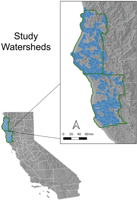
Figure 1. Study area map. humboldt and mendocino Counties are outlined in green and contextualized within the state of California. Study watersheds are depicted in blue. The scale bar corresponds to the inset map.
Download figure:
Standard image High-resolution imageWater extraction modeling
We developed a modeling framework for predicting monthly water extraction volumes for cannabis cultivation in northern California, using water-use reporting information from permitted farms and geospatial data describing farm size, location, and operational characteristics (figure 2). Annual and monthly water totals were obtained from reporting data submitted by permitted cannabis farms enrolled in the CWB cannabis program. Because the data were self-reported, only farms using water meters or known application rates (i.e., emitter rates applied to watering schedules) were included in the analysis. As described by Dillis et al 2020, water extraction was considered separately from water demand. While water demand reflects the total annual amount of water a cannabis farm needs to grow their crop, water extraction reflects when this water is actually withdrawn from the environment, including water diverted to storage and directly applied to plants. Extraction volumes are therefore considered a more ecologically relevant metric of water consumption by cannabis farms. Monthly estimates of water extraction volumes were generated by first modeling annual water demand and then applying a monthly water extraction profile model to estimate how annual demand was extracted over the year (Dillis et al 2020). We then applied the models to farm mapping data for the region to estimate the monthly extraction volumes for all farms in the sampled watersheds, including both permitted and unpermitted farms. Each step in the modeling framework is described in detail below.
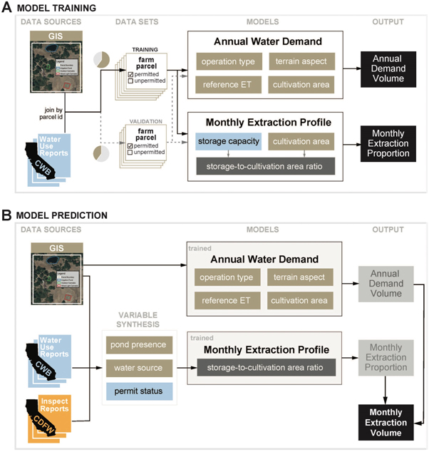
Figure 2. Model training and prediction workflow. Data sources, models and outputs are summarized for both model training (A) and model prediction (B). Variables in models are color-coded to correspond to their original source. Model training includes a diagram of the training and validation data sets, which were both applied to the annual water demand and monthly extraction profile models. For model prediction, the synthesis of the storage-to-cultivation area ratio variable is depicted in which GIS is used to establish whether a farm has a pond and/or a well, and CWB permit records are used to determine whether it is permitted or unpermitted. CWB water use reports and CDFW inspection reports are used to determine the average STCA Ratio values for permitted and unpermitted sites (respectively), based on the presence/absence of ponds and wells. These average values constitute the STCA Ratio values to be used in the monthly extraction profile model.
Download figure:
Standard image High-resolution imageAnnual water demand
We first developed an annual water demand model, relying on data from permitted farms from 2018–2020 (n = 1,161). Data from CWB annual reports included cultivation area, operation type(s), and a monthly reporting of water use, which was summed for each farm to serve as the annual water demand response variable. We reviewed 2018 and 2020 NAIP aerial imagery to digitize cultivation area for each CWB farm instead of relying on reported values. Because many farms have both mixed-light and outdoor cultivation areas, we quantified operation type as the proportion of outdoor cultivation present at a site. Two additional variables were generated for each farm as predictors of annual water demand: reference evapotranspiration (ET) and terrain aspect, which were obtained from the TerraClimate dataset (Abatzoglou et al 2018), available in Google Earth Engine (Gorelick et al 2017), and Digital Elevation Models (DEMs) from the National Elevation Dataset (USGS 2020), respectively. Reference ET was calculated as an average daily value during the growing season (April - October) and was chosen to represent climatic conditions, as it encompasses surface temperature, relative humidity, and other factors that otherwise introduce collinearity if considered as separate predictors. Terrain aspect was calculated as the average parcel value (0°–360°), which was recentered to South aspect (180°) by subtracting 180 and taking the absolute value (thus South becomes 0°, East and West both become 90°, and North becomes 180°). The source data used to calculate terrain aspect were finer resolution (30 m raster cell) than reference ET (4638.3 m raster cell), thus making it more sensitive to microclimatic variations.
Four separate models were fit and compared using R statistical software (R Core Team 2018) to select a top-candidate annual water demand model (appendix A). Candidate models included: (1) a rate-based estimate (i.e., m3 m−2) relating cultivation area to annual water demand, (2) a simple Ordinary Least Squares (OLS) model using cultivation area and operation type as predictors of water demand, (3) an enhanced OLS model that also included reference ET and terrain aspect, and (4) a generalized linear model similar to that used by Dillis et al 2020 with cultivation area, operation type, reference ET, and terrain aspect as predictors. For each model, a training set (random subsample of 60% of the dataset) was used to make predictions for the reserved test set (remaining 40% of the dataset) and performance was assessed over 1,000 validation iterations. Although there were multiple years of data used in the analysis, training and test sets were split by farm ID so that no farms were used to make predictions for themselves in subsequent years. Model predictions for the test sets and their observed annual water demand values were compared, using percent bias, Mean Absolute Error (MAE), and r2 to select the top performing model (with priority to the three metrics following the order listed). Comparisons were based on 100 iterations of training and test sets for each model.
The top performing model was the enhanced OLS regression using all of the predictor variables described above (appendix A). The model structure can be described as:

where, Wi is estimated water demand volume of a farm (i) in cubic meters, as a function of cultivation area (c), operation type (t), reference ET (v), and terrain aspect (r), as well as interaction terms for cultivation area and operation type (ct), cultivation area and reference ET (cv), and cultivation area and terrain aspect (cr). Water demand is modeled as a linear combination of these variables, fit with slope coefficients (β) and an intercept term (α). Huber-White robust standard errors were calculated to account for heteroskedasticity (figure S1), using the sandwich and lmtest packages in R (Zeileis and Hothorn 2002, Zeileis 2006).
Monthly extraction estimation
In the second step of the modeling framework (figure 2), we partitioned annual water demand into monthly estimates based on an extraction profile model. Data from 2017–2018 water reports for permitted farms (n = 1,130) were used for determining monthly proportions of water extraction. This period predates seasonal water use regulations adopted in 2019, which prohibit the diversion of surface water for the duration of the growing season (April-October). We therefore assume that water use practices by permitted farms prior to 2019 are representative of unpermitted farms with otherwise similar operation types and site characteristics. We used the water storage capacity of farms to model monthly extraction profiles, given that storage capacity has been shown to be a primary determinant of seasonal water extraction timing (Dillis et al 2020). We normalized storage capacity by cultivation area to calculate a storage capacity to cultivation area ratio (hereafter, STCA ratio), using data from the CWB annual reports. We then fit a multinomial model to estimate the likelihood each observation of water extraction (aggregated into discrete 3.79 m3 (1,000 gallon) units for each monthly reported total) occurring in a given month (M), based on the STCA ratio (s) of the farm (i) at which it occurred. The multinomial logit structure of the model ensured that all monthly likelihood estimates summed to unity. Monthly likelihoods were therefore interpreted as the monthly proportions of total annual water extraction. A generalized linear model was fit using the nnet package (Venables and Ripley 2002) in R statistical software. The model structure can be described as:

where an intercept term (α) is added to the storage ratio term (βs ) to produce a log-odds estimate of the likelihood of a water extraction observation occurring in a given month. Log-odds estimates were converted to monthly likelihoods prior to multiplying them by the annual demand estimates in order to generate monthly extraction volume estimates. The predictive performance of the entire composite model was analyzed on a monthly basis, using the same process and criteria (MAE, percent bias, r2) as described for the annual demand models.
Cumulative and relative water extraction volumes for permitted and unpermitted farms
We next applied the water demand models to all farmed parcels in the study watersheds (figure 1). For each farmed parcel (permitted and unpermitted), we calculated the cultivation area and operation type variables using 2018 NAIP aerial imagery. We also calculated reference ET and terrain aspect for all farmed parcels, as described above. We then used the trained model from equation (1) to predict annual water demand at all farms with the calculated explanatory variables. To estimate the monthly extraction volumes of cannabis farms, we first determined whether an irrigation pond was present and estimated the likelihood that there was access to groundwater at the site. These factors have been previously shown to strongly influence the seasonal patterns of water extraction at cannabis farms (Dillis et al 2020). Specifically, farmers who rely on groundwater wells tend to employ limited or no long-term water storage and thus have water extraction profiles that track the water needs of cannabis (i.e., water is extracted and applied on demand). In contrast, farmers who rely on surface water tend to have more water storage, as these sources tend to be more ephemeral (and are subject to seasonal use restrictions), and therefore extract water in the winter months, outside of the growing season. Farms that have access to large on-site storage, such as an irrigation pond, extract most of their water in the wet season, such that water extraction is out-of-phase with plant demands (Dillis et al 2020).
Aerial imagery for each farmed parcel was inspected to determine the presence of an irrigation pond. To determine whether or not farms had access to groundwater, we used a classification model described by Dillis et al (2021b) that relies on water source information from permitted farms (n = 1,237) in Humboldt and Mendocino County. The model used 13 variables describing the local topographic, climate, and watershed characteristics of farm locations (table S3) to make a categorical prediction of farm reliance on groundwater (i.e., well/no well). All farm-level model parameters were generated from open-source GIS data, including Digital Elevation Models (DEMs) from the National Elevation Dataset (USGS 2020), watershed boundary and stream flowline data from the National Hydrography Dataset (USGS 2019), and precipitation data (30-year annual average) from the PRISM Climate Group (PRISM Climate Group 2018). The model was trained with source-water information at permitted sites and tested against CDFW inspection data from unpermitted farms for which a water source was recorded (n = 80), which demonstrated an acceptable level of accuracy (71.75%) and bias (+2.65%).
Based on the observed presence of irrigation ponds and predicted well use, all farms in the study area, including permitted and unpermitted farms, were assigned to one of four categories: (1) those with wells, but without ponds, (2) those without wells and ponds, (3) those without wells and with ponds, and (4) those with wells and ponds. Each of these farms was then assigned a STCA ratio based on the mean values calculated for permitted and unpermitted sites within each respective category, using CWB reporting data and CDFW inspection data. STCA ratio values were then used in the water extraction profile model to estimate the monthly proportion of water extraction, and subsequently applied to estimated annual demands, to produce monthly extraction volumes at all farms in the study area. Monthly water extraction volumes for permitted and unpermitted farms were then aggregated by watershed (HUC12).
To provide context for cannabis water extraction estimates, monthly instream flow estimates were calculated for each study watershed using a natural flow model described by Zimmerman et al (2018). Mean monthly natural flow estimates were generated for each outlet stream segment of study watersheds, converted from cubic feet per second to cubic meters per month, and compared against cannabis water extraction estimates. We specifically evaluated water extraction volumes relative to natural water supply volumes during the peak growing season (July—September).
Scenario modeling
Finally, we used our modeling framework to explore how dry season (July-September) water extraction demands for the region might change under alternative future policy scenarios. We considered hypothetical scenarios to compare the efficacy of management approaches used to reduce summer water extraction: prohibiting surface water diversions in the dry season, expanding storage capacity (to allow for capture of more water in the wet season), and implementing both strategies simultaneously. The first policy scenario, Full Compliance, considers a future in which unpermitted farms become permitted and all cannabis cultivators comply with seasonal forbearance regulations under existing policy, which prohibits surface water diversions between April and October. For this scenario, all unpermitted farms that rely on surface water were assigned to a monthly extraction profile in which all water demands are met by surface water diversions in the wet season (i.e., by storing water). A second scenario, Median Storage, was used to represent a future in which all cannabis farms (permitted and unpermitted), regardless of water source, expand their storage capacity to the median STCA ratio value reported by permitted farms. This represents a plausible level of potential increased storage capacity for farms, while recognizing the logistical and financial challenges of storage expansion (Dillis et al 2020). To represent a less ambitious storage target, we also considered a 25th Percentile Storage scenario, in which all farms have access to storage equivalent to the 25th percentile of the STCA ratio of permitted farms. A final scenario, Combination, was also considered to represent a future in which all farms comply with the forbearance requirement but also expand their storage capacity to the median STRA ratio value. We re-ran the models with the revised farm attributes from each scenario and calculated the percent change in dry season water extraction volumes for all watersheds in the study region.
Results
Water extraction modeling
The OLS model with reference ET and terrain aspect performed best in predicting annual water demand relative to the other model configurations (MAE = 303.12 m3; Pbias = 0.10%; r2 = .34; table S2). The enhanced OLS annual water demand model (table 1) showed reliable interactions between cultivation area and the three other predictor variables operation type (MLE = −0866; SE = 0.0292), reference ET (MLE = 0.003; SE = 0.001), and terrain aspect (MLE = −0.016; SE = 0.003), indicating that their effects are amplified with increasing values of cultivation area (figure 3). Although a simpler OLS model did not perform as well in predicting annual water use, the model coefficients are included as supplementary material (Table S4). This model provides a method for estimating annual water demand from a cannabis farm that does not require processing reference ET or terrain aspect data, yet performed only slightly worse than the enhanced OLS model and was superior to the rate-based model (table S2).
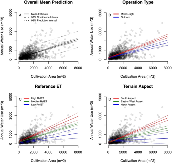
Figure 3. Annual water demand model predictions. predictions from the enhanced OLS model for annual water demand are plotted over raw data as an overall prediction (A) and for each of the three variables: operation type, reference evapotranspiration, and terrain aspect. Separate predictions for mixed-light (proportion outdoor = 0) and outdoor (proportion outdoor = 1) operation types are depicted (B). Predicted values for reference evapotranspiration include the median, as well as the highest and lowest values of the range (C). Predicted values for average terrain aspect combine East and West, as they are considered equivalent by the model (D).
Download figure:
Standard image High-resolution imageTable 1. Maximum Likelihood Estimates for the top performing annual water use model (enhanced OLS model).
| Coefficient | MLE | SE |
|---|---|---|
| Intercept | −197.3406 | 257.2038 |
| Cultivation Area | −.0498 | 0.1393 |
| Operation Type | −23.2003 | 52.4324 |
| Ref Evapotranspiration | 0.2511 | 0.1989 |
| Terrain Aspect | −1.0402 | 0.6284 |
| CA*OT Interaction | −0.0866 | 0.0292 |
| CA*RE Interaction | 0.0003 | 0.0001 |
| CA*TA Interaction | −0.0016 | 0.0003 |
In the extraction profile model, variation in the STCA ratio resulted in strongly divergent monthly extraction patterns (figure 4), consistent with Dillis et al 2020. Coefficient estimates (table 2) demonstrated that relative to January (reference level), the summer months of July (MLE Intercept = 2.08, SE = 0.03), August (MLE Intercept = 2.23. SE = 0.03), and September (MLE Intercept = 1.97, SE = 0.03), were reliably predicted to experience the greatest proportion of annual water extraction. Coefficient estimates for the STCA ratio were reliably negative and most strongly negative in the summer months (July MLE = −13.38, SE = 0.27; August MLE = −14.48, SE = 0.28; September MLE = −13.77, SE = 0.29), reflecting that with increasing amounts of water storage, less water is extracted during this period of the year. Of the four farm typologies, those using a well and that did not have a pond for storage had the lowest STCA ratio and the highest predicted proportion of water extraction in July (18%), August (20%), and September (16%). By contrast, farms without wells, but with an irrigation pond had the highest predicted proportion of water extraction in January (21%), February (22%), and March (21%).

Figure 4. Monthly extraction profiles. model estimates for monthly proportion of annual demand, based on STCA Ratio. Predicted monthly values are overlaid on the interquartile range of the raw data (depicted as vertical bars) for each of the four farm types for permitted farms: (A) Well/No Pond, (B) No Well/No Pond, (C) No Well/Pond, (D) Well/No Pond. Model predictions for each farm type are also provided for unpermitted farms, based on STCA Ratios from unpermitted farm data (F-H). Dashed lines indicate the 95% confidence interval of the mean estimates. The 95% confidence interval for January was constructed using a separate binomial comparison (January versus all other months) to produce standard errors.
Download figure:
Standard image High-resolution imageTable 2. Monthly water extraction profile model. Multinomial model coefficients are provided in bold. Standard errors are provided in parentheses. Model predictions based on maximum likelihood estimates are produced for each combination of predictor variables and for each month. Model coefficients were not calculated for January, as it was the reference level for multinomial comparisons against all other months.
| Month | Intercept | STCA Ratio | Monthly Proportion: | Monthly Proportion: | Monthly Proportion: | Monthly Proportion: |
|---|---|---|---|---|---|---|
| Well/No Pond | No Well/No Pond | No Well/Pond | Well/Pond | |||
| Jan | ref | ref | .03 | .12 | .21 | .21 |
| Feb | 0.05 (0.03) | 0.00 (0.04) | .04 | .12 | .22 | .22 |
| Mar | 0.01 (0.03) | 0.00 (0.04) | .04 | .12 | .21 | .21 |
| Apr | −0.05 (0.03) | −0.81 (0.07) | .03 | .09 | .10 | .10 |
| May | 0.69 (0.03) | −3.93 (0.14) | .06 | .10 | .02 | .02 |
| Jun | 1.70 (0.03) | −11.00 (0.25) | .13 | .06 | .00 | .00 |
| Jul | 2.08 (0.03) | −13.38 (0.27) | .18 | .06 | .00 | .00 |
| Aug | 2.23 (0.03) | −14.48 (0.28) | .20 | .05 | .00 | .00 |
| Sep | 1.97 (0.03) | −13.77 (0.29) | .16 | .05 | .00 | .00 |
| Oct | 1.03 (0.03) | −6.70 (0.20) | .08 | .08 | .00 | .00 |
| Nov | −0.51 (0.04) | −0.42 (0.07) | .02 | .06 | .09 | .09 |
| Dec | −0.46 (0.04) | 0.21 (0.05) | .02 | .08 | .16 | .16 |
Predictive performance of the composite model (annual demand and monthly extraction) varied across months and was generally best during the growing season (May through October; table 3). While MAE was mostly consistent across most months, percent bias was notably lower in July (6.00%), August (3.20%), and September (4.80%) than in the off-season months of November (109.00%), December (96.90%), and January (79.90%). The r2 values were also higher in the months of July (r2 = 0.36), August (r2 = 0.35), and September (r2 = 0.34) than in November (r2 = 0.08), December (r2 = 0.11), and January (r2 = 0.14). This discrepancy in model performance was likely due to the fact that water extraction in the offseason is being input to storage and can vary by farms based on local water availability and diversion schedules. Additionally, offseason water extraction (November through April) often involves input to irrigation ponds, the capacities of which can include extreme outliers that the model cannot account for. Predictive performance of the composite model in the offseason months was considerably improved as outlier values of reported water extraction were removed (appendix A).
Table 3. Monthly predictive performance of the composite annual demand and monthly extraction models.
| Month | MAE | Bias (%) | r2 |
|---|---|---|---|
| January | 60.99 | 79.90 | 0.14 |
| February | 48.97 | 40.70 | 0.38 |
| March | 61.77 | 72.90 | 0.12 |
| April | 45.32 | 65.90 | 0.06 |
| May | 33.82 | 10.90 | 0.09 |
| June | 35.18 | 3.90 | 0.33 |
| July | 44.24 | 6.00 | 0.36 |
| August | 48.87 | 3.20 | 0.35 |
| September | 40.91 | 4.80 | 0.34 |
| October | 35.95 | 19.30 | 0.06 |
| November | 45.72 | 109.00 | 0.08 |
| December | 50.71 | 96.90 | 0.11 |
Cumulative and relative water extraction for permitted and unpermitted farms
Farm-level estimates for all mapped permitted (n = 823) and unpermitted (n = 5,959) farms, generated by the composite water extraction model, were aggregated at the watershed scale. The number of unpermitted farms (Median = 9; IQR = [3, 47] and associated cultivation area within watersheds (Median = 0.021 km2; IQR = [0.006, 0.047) was typically greater than permitted farms (Median number = 1; IQR = [0, 7]; Median size = 0.003 km2; IQR = [0.000, 0.013]). There was also noticeable spatial divergence between watersheds in terms of permitted and unpermitted cultivation (figures 5(A) and (B)), with some primarily supporting permitted farms and others primarily supporting unpermitted farms. The distribution of overall (permitted and unpermitted) water extraction totals reflected these differences and varied by orders of magnitude between watersheds (figure 5(C)) and primarily tracks the pattern of unpermitted cultivation given its larger presence on the landscape. That is, the watersheds with the highest annual water extraction totals are those with the largest footprint of unpermitted cannabis cultivation.

Figure 5. Map of cultivation area and water use. watershed level summaries of hectares of permitted (A) and unpermitted (B) cannabis cultivation are accompanied by overall water extraction total estimates during peak water extraction months (July through September; (C). Percentage of water extraction relative to instream flow during peak extraction months is provided for context (D).
Download figure:
Standard image High-resolution image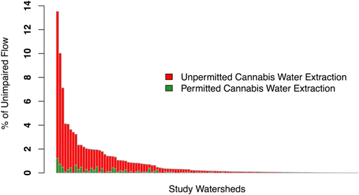
Figure 6. Water extraction versus instream flow. Watersheds are sorted by the percentage of available instream flow used by cannabis water extraction during the peak months (July through September). Percentage estimates are divided into unpermitted (red) and permitted (green) cannabis water extraction.
Download figure:
Standard image High-resolution imageDifferences in extraction profiles of permitted and unpermitted farms were most pronounced for farms without wells or ponds. Unpermitted farms of this typology had STCA ratio values (0.01) much smaller than permitted farms (0.21), demonstrating more on-demand extraction during the summer months (figure 4(A)) by the former. By contrast, there was little difference between permitted and unpermitted farms that relied on groundwater, as both had relatively low STCA ratios (0.03; 0.01), and thus extracted water on demand. As a result, differences between permitted and unpermitted water extraction patterns were amplified in areas where farms were predicted to rely more on surface water than groundwater. Differences between permitted and unpermitted extraction volumes were most pronounced in the dry season (figure 7). For example, differences in July (Median = 1120.83 m3 km−2; IQR = [356.05, 2898.83]), August (Median = 1285.48 m3 km−2; IQR = [411.40, 3327.11]), and September (Median = 1002.77 m3 km−2; IQR = [319.43, 2594.22]) were much larger than in November (Median = 166.67 m3 km−2; IQR = [45.71, 453.66]), December (Median = 261.69 m3 km−2; IQR = [63.32, 691.66]), and January (Median = 351.54 m3 km−2; IQR = [90.39, 954.05]).
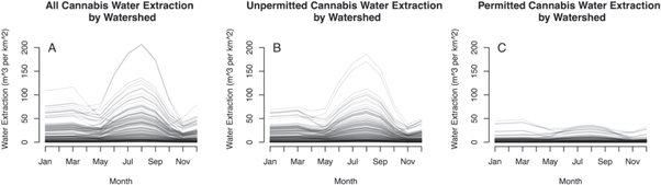
Figure 7. Monthly watershed extraction estimates. Cumulative (A) and relative magnitude and timing of unpermitted (B) and permitted (C) water extraction (normalized by watershed area) is depicted on a monthly basis, with each line representing a single watershed.
Download figure:
Standard image High-resolution imageMost of the water extraction associated with unpermitted farms was concentrated in a small subset of watersheds (figure 8). Almost one third of all unpermitted water extraction was attributed to 10 of 115 study watersheds (8.6%) on both an annual basis (32.93% of total unpermitted extraction) and during the peak water extraction period (July - September; 33.21% of total unpermitted extraction). The unpermitted water extraction in these 10 watersheds also accounted for over one quarter of all (permitted and unpermitted) estimated water extraction in the study area on both an annual basis (26.59%) and in the peak water extraction period (28.53%).

Figure 8. Distribution of water extraction among watersheds. Histograms comparing the area-normalized watershed water extraction totals by permitted and unpermitted cannabis on an annual basis (A), as well as during the peak water extraction month of August (B).
Download figure:
Standard image High-resolution imageWe found that cannabis water demand for the peak growing season (July—September) was estimated to represent a small percentage of naturally available surface-water supplies, when evaluated at the HUC12 watershed scale (figure 6). Estimated percentages did not exceed 1% of estimated instream flow in 89 of 115 watersheds and only exceeded 2% in 12 of 115 watersheds. The largest estimated value for a single watershed was 13.53%. Spatial patterns in cannabis water extraction expressed relative to water availability tracked the distribution of unpermitted cannabis (figure 5(D)), reflecting the disproportionate amount of water used by unpermitted cannabis in the dry season.
Scenario modeling
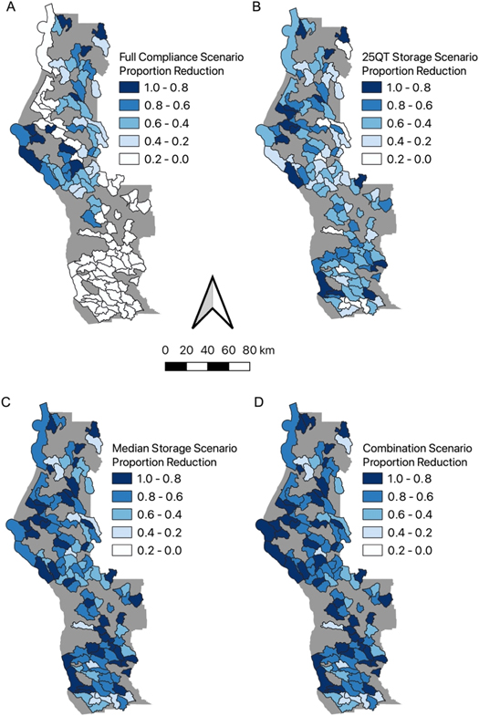
For the Full Compliance scenario, in which all farms in the study area were assumed to comply with seasonal surface water diversion restrictions, water extraction during peak summer months was reduced in most watersheds (July-September; figure 9). Water extraction was reduced by 50% or more in 34 watersheds under the Full Compliance scenario. However, in the majority of watersheds (63 of 115), dry season water extraction was reduced by less than 25% relative to the current extraction estimates. This is because many of the farms in these watersheds rely on groundwater wells and are not subject to dry season forbearance requirements. Enhancing water storage capacity had a more significant effect on dry season extraction estimates. Under the Median Storage scenario, 112 of the 115 study watersheds were estimated to have water extraction reductions of 25% or more, with estimated reductions of 50% or greater in 96 of 115 watersheds. Notable reductions in extraction volumes were also estimated under the 25th Percentile Storage scenario, in which 103 of 115 watersheds were estimated to have reductions of 25% or more, with estimated reductions of 50% or greater in 60 of 115 watersheds. The Combination Scenario, which assumed farms would both enhance storage and forbear from surface water diversions in the dry season, produced the largest reductions in summer water extraction, with 100 of 115 watersheds having reductions of 50% or more and 112 of 115 watersheds having reductions of 25% or more.
Figure 9. Scenario modeling. the estimated reductions for each watershed are displayed under the four scenarios (A) Full Compliance, (B) 25th Percentile Storage, (C) Median Storage, (D) Combination.
Download figure:
Standard image High-resolution image
Discussion
The current study is the first to utilize reported water storage and use data to estimate annual and monthly water extraction volumes for both permitted and unpermitted cannabis farms in California. Although the data used to estimate water demands were self-reported, they represent the largest dataset on cannabis water-use practices currently available. Despite statewide legalization of cannabis, we found that unpermitted cannabis farms in the region continue to have a greater water footprint than permitted farms and remain a concern for their potential impacts to sensitive freshwater resources (Bauer et al 2015, Carah et al 2015).
The study demonstrated that variation in farm characteristics, including operation type, climate, and topography, can lead to significant differences in annual water demands. We also found that even a simple linear model represents a substantial improvement to rate-based models, which assume that water consumption by cannabis farms scales linearly with cultivation areas (with a zero-intercept). Such rate-based models significantly overpredict annual water demand, especially at large farm sizes (figure S1), while the simple linear model (with a non-zero intercept) demonstrates limited bias in over or underestimating annual water use. Finally, we demonstrated that annual demands can be partitioned into monthly extraction estimates through the use of multinomial models that consider only the water storage capacity at a site. The limited data available on the storage capacity of unpermitted farms likely introduces some uncertainty in model predictions because only a small proportion of unpermitted sites have been subject to CDFW inspections. As a result, the total capacity of small tanks, bladders, and other storage infrastructure commonly used by cannabis farms, but that are not easily detected in aerial imagery, is difficult to estimate. Nevertheless, the strong performance of the model (trained with permitted data and tested against independent data from unpermitted sites) indicates that it is a reliable approach for estimating monthly cannabis water demands and represents a marked improvement over existing methods currently used by government and industry stakeholders.
Reducing summer water extraction
Unpermitted water extraction is responsible for a disproportionately large share of total water consumption by cannabis agriculture in Northern California and this difference is magnified in the driest months of the year when streamflow is lowest (Bauer et al 2015, Carah et al 2015). Based on estimates of water extraction relative to instream flow, our results indicate that cannabis water demands are likely more of an issue at the scale of smaller headwater streams than over an entire watershed. Permitted farms typically have access to water storage to collect irrigation water in wet season months, thereby (at least partially) limiting surface water diversions in drier periods. However, our results suggest that storage capacity of unpermitted farms is more limited, resulting in relatively higher dry season extraction proportions. Given the higher number of unpermitted farms in the region and greater cultivation footprint, dry season demands by unpermitted farms in the region remains a potentially significant pressure on water resources in the region.
Our scenario analyses suggest that there are opportunities to reduce the amount of water extraction from watersheds in the dry season, including transitioning unpermitted farms to the regulated industry to comply with seasonal forbearance requirements as well as the expansion of on-site water storage capacity at both permitted and unpermitted sites. The spatially clustered nature of unpermitted farms suggests that highly impacted watersheds may be valuable targets for outreach efforts aimed at transitioning unpermitted farms to the regulated industry. Campaigns to increase water storage capacity are also likely to be helpful in reducing dry season water demands at both permitted and unpermitted farms. Our scenario modeling demonstrated that the most effective and widespread reduction in summer water extraction would occur if all farms implemented a moderate amount of storage. An additional avenue by which water extraction may be reduced, but not examined in this study, is through improvements in water use efficiency, thereby decreasing demand. The broad range of annual water use values (normalized by cultivation area) we observed suggest that some cannabis farms are using substantially more water than others. Horticultural research to produce a crop coefficient for cannabis, as exists for nearly every other agricultural crop, would give farmers a better sense of at what point crops are being overwatered and no longer using all of the irrigation water they are allocated.
Estimating potential streamflow impacts
A robust assessment of cannabis water-use impacts on streamflow requires improvements in estimation of instream water availability, characterization of subsurface hydrogeologic properties, and quantification of other anthropogenic water uses. The impacts of cannabis cultivation are most likely to occur in small headwater streams (Bauer et al 2015), which rarely have gaging stations, making it difficult to directly measure streamflow responses. However, recent advances in the use of machine learning models (e.g., Grantham et al 2022) and other hydrologic modeling methods have improved the accuracy in predicting flows in ungaged streams. The strategic placement of new gages, coupled with improved models, would be helpful for developing reliable estimates of streamflow in cannabis-producing watersheds. This study reinforced previous findings by Dillis et al 2021 documenting that many cannabis farmers in Northern California are relying on groundwater wells to meet their irrigation needs. Extraction from groundwater wells can have similar effects as direct surface water diversions, although the timing and magnitude of streamflow depletion is strongly affected by subsurface soil properties (Zipper et al 2019). For example, Hahm et al 2019 demonstrated that watershed lithology can have a significant effect on subsurface water storage and streamflow characteristics in Northern California streams. In particular, watersheds underlain by weathered bedrock (agrillite and sandstone) in the Coastal Belt have greater storage capacity than those dominated by the Central Belt mélange (argillite matrix) (Langenheim et al 2013, Hahm et al 2019). As a result, streams overlaying Central Belt lithology tend to be flashier, tracking patterns of seasonal rainfall, and often dry in summer, which could make them more sensitive to streamflow depletion from water diversions. In contrast, Coastal Belt streams are often sustained by subsurface flows throughout the dry season (Hahm et al 2019) and the greater storage capacity could make them less sensitive to both groundwater and surface water withdrawals.
In addition to considering the irrigation water source and hydrologic properties of the watershed, estimation of streamflow impacts in cannabis-producing watersheds must consider the influence of other water users, which have demands that often exceed those of cannabis. For example, Zipper et al 2019 reported that water extraction for residential use contributed more to streamflow depletion than cannabis in another northern California watershed. Finally, to improve estimation of potential streamflow impacts additional data from both permitted and unpermitted farms are also needed to better characterize water use efficiency, storage capacity, and water extraction volumes. For example, field observations of unpermitted farms by CDFW staff frequently document sources of water waste including leaking pipes, overflowing passive inputs to water tanks, and unlined irrigation ponds. Understanding the extent to which these types of waste characterize water use practices is critical for developing water-use efficiency standards and promoting strategies to limit streamflow depletion risk.
Conclusions
Although the permitted cannabis industry continues to grow in California (Dillis et al 2021b), the persistent and disproportionate representation of unpermitted cannabis farms highlights the need to consider their distinct and collective water-use footprints. Estimating the impact of cannabis cultivation on streams that support sensitive freshwater species and other beneficial uses first requires accurate accounting of the timing and volume of water extracted from surface and groundwater. Here, we identify potential strategies to limit dry season demands in the dry season and mitigate environmental risks, including efforts to transition unpermitted farms to the legal market and those to enhance storage capacity on both permitted and unpermitted forms. Small, unpermitted cannabis farmers have reported that their decision to remain in the illicit industry is related to high compliance costs and competition from much larger operations, rather than avoidance of environmental regulations (Bodwitch et al 2021). Thus, programs that incentivize expanded off-stream storage capacity in order to limit potential environmental impacts may be most effective in the short-term and are likely to be well-received by unpermitted and permitted growers alike. This is especially true given increasing water security risks (Morgan et al 2021) and growing wildfire threats (Dillis et al 2022) facing cannabis cultivators in the region.
Acknowledgments
This work was made possible in part through funding from the California Department of Fish and Wildlife, the Resources Legacy Fund, and the Campbell Foundation. We thank Jennifer Natali for help with figure production. We are also thankful for the work of over 20 undergraduate students who digitized cannabis cultivation sites in Humboldt and Mendocino Counties.
Data availability statement
The data generated and/or analysed during the current study are not publicly available for legal/ethical reasons but are available from the corresponding author on reasonable request.
Supplementary data (0.3 MB PDF)