
Abstract
Graphene and carbon nanotube (CNT) have been proposed to be good materials for thermionic energy converter (TEC). For accurate simulation of performance of TEC, it is important to know the correct equation for temperature dependence of thermionic emission current density (J) from graphene and carbon nanotube. In this paper we first consider the existing theory of electron energy dispersion relation in graphene to reconsider the relations between Fermi energy and Fermi velocity in relation to some form of electron mass in graphene. We then consider existing various models of temperature dependence of J versus T (J(T)) and their applicability to nano-materials. We find that no model exists to date that fully conforms to the available experimental data on J(T) of nano materials. By providing justifications for three components of electron momentum vector during thermionic emission from graphene, we then find a three-dimensional model that fits the experimental thermionic emission data from graphene and carbon nanotube far better than any existing model. We present a detailed comparison of our model with existing models of thermionic emission. The work function determined using our model also agrees very well with independent experimental results. This model is expected to be very effective in modelling TEC with graphene or CNT.
Export citation and abstract BibTeX RIS

Original content from this work may be used under the terms of the Creative Commons Attribution 3.0 licence. Any further distribution of this work must maintain attribution to the author(s) and the title of the work, journal citation and DOI.
1. Introduction
Thermionic emission of electrons played a key role in advancement of Physics, electronics and many areas of modern science and technology. The equation for the current density (J) of emitted electrons at temperature T is so far given by the well-known Richardson-Dushman Equation:

A0 is the well-known Richardson-Dushman constant is  where W is the work function of the material and kB is the Boltzmann constant. The equation known as RD law can be derived following Sommerfield's model [1] of three-dimensional free electron gas in a metal.
In recent years, thermionic electron emission and field electron emission from low-dimensional nanostructures, e.g. carbon nanotubes (CNTs), graphenes, etc, have been widely studied experimentally [2–9]. To interpret the measured emission current density from low-dimensional nanostructures, the macroscopic Richardson-Dushman law and Fowler–Nordheim law were usually directly applied in previous reports [3, 4, 6–8]. Like carbon nanotube (CNT) [4–6] the electron emission processes (field and photo-assisted over-barrier electron emission) from graphene [7, 8] seem to require revisions of existing law (Richardson-Dushman (RD)) to account for unique properties of graphene. Some recent works [2, 3] question the validity of the RD law [9] in graphene [2, 3, 10] and CNT [11, 12] while some indicate the validity [13]. In recent years thermionic emission from carbon nanotubes and graphene has received special attention [14–20] still questions remain about the validity of the RD law in these materials. Wei et al. [21] carried out very careful measurements of thermionic emission current density from many individual CNTs and examined the validity of the RD law in details for each of them. They found that the plot of  versus
  showed an upward bending instead of giving a straight line as required by the RD law. Thus, they concluded that RD law breaks down for the thermionic emission from individual CNTs. Sherehiy [22] carried out studies on 'Thermionic emission properties of novel carbon nano-structures' and determined work functions of different nano-structures from the data on thermionic emission current density at different temperatures, reduced to zero Schottky effect. They had an interesting discovery – nanostructures with lower surface charge density have higher work function- which was qualitatively explained to be due to different density of states.
Since the discovery of exfoliated mono-layer graphene [23] in 2004, graphene has exhibited many unique properties such as: linear band structure [24], ultra-high mobility high thermal and electrical conductivity [24]. Graphene is typically referred to a single atom thick layer of carbon, although sometimes bilayer or trilayer graphene are also mentioned. Graphene is a two-dimensional (2D) material, formed of a hexagonal lattice of carbon atoms which are covalently bonded in the plane by sp2 bonds between adjacent carbon atoms. The bonding energy (approximately
  ) between adjacent carbon atoms is among the highest in nature (slightly higher than the sp3 bonds in diamond) [25]. With a single-atom-thick sheet of sp2 -hybridized carbon atoms, graphene exhibits great promises for future applications in energy storage [26], nanoelectronics [27, 28], and composites [29]. With the high bond strength among the adjacent in-plane carbon atoms thus graphene is a material for high temperature devices [30] (operating in vacuum) and thus has a potential for a suitable candidate as an emitter in a thermoelectronic [with no ions involved] energy converter [TEC].
In a TEC [31–34] with the work function of the emitter,  of the anode (collector) and when the emitter and collector is connected through a load, the output power is
  where Ie and Ic are the emitter and collector emission currents. The latter quantities are primarily controlled by temperature and work functions of emitter and collector
  the emitter collector configuration (i.e., the space between them), and arrangements that control space charge. Recently Yuan et al. (2017) discussed new method of controlling space charge using magnetic field and gate voltage [34]. To model a TEC, specially, with graphene as an emitter, it is very important to obtain the accurate model of temperature dependence of
  It may be mentioned that thermionic energy converter (TEC) once perfected can store the electrical energy by charging a battery with circuits similar to that of solar panel. It will reduce the dependence on silicon.
Liang and Ang [2, 3] have fitted J versus T data from monolayer two dimensional graphene [35] by developing a thermoelectronic emission equation, different from that of RD law, assuming massless Dirac electron inside graphene. In their theory they have considered Fermi energy and Fermi velocity of electrons in graphene to be two independent parameters. As shown below this concept contradicts the current understanding of electron dynamics in graphene. Apart from this their theory has many errors from physics and mathematics point of view as pointed out in [36].
Moreover, they did not consider the variation of work function with temperature (T) in the thermionic emission equation, which our present work shows to be very important, specially, when the Fermi energy at 0 K,  is low, as it is in graphene. It has not been known whether their theory applies for the CNT. Moreover, in the light of experimental discovery [37] of finite dynamic electron mass and the attribution of some form of mass to electrons in graphene based on the current concept of electron dynamics as given below, their model becomes questionable. Thermionic emission involves electron dynamics and hence dynamic electron mass or some form electron mass in graphene should apply. Otherwise, the fundamental question how electrons acquire mass when emitted from graphene, if their effective mass is zero in graphene. Moreover, in fitting the experimental J versus T data for monolayer graphene they had assumed the Fermi group velocity, VF to be
  while more recent experimental works show it to lie in the range
  to
to  For monolayer graphene the latter value applies. As discussed later VF affects significantly the fitting of the experimental data.
There are thus challenges in a correct formulation of the theory of electron emission from graphene and CNT. Below we consider a few possible models for thermionic emission from graphene briefly without giving the elaborate derivations of the models because of space. Then we provide first brief outline of the existing theory of electrons in graphene. This shows that electrons are not truly massless as conjectured by many earlier. Then we present our own simple model which is seen to fit the experimental data of thermionic emission from both graphene and carbon nanotube.
2. Brief outline of different possible models of thermionic emission from graphene
In graphene, if one considers emission from graphene edge, the emission may be treated like that of Somerfield model except the fact that the density of states in a two-dimensional material is independent of energy. Such treatment has been recently conducted by Wei et al. [11]. Moreover, as the expected net current from edge is quite low, edge emission may not be of quite practical interest. However, while treating the emission perpendicular to the graphene sheet (i.e., along the z-direction from the surface) one must consider the quantum confinement effect along z, which can be done in the line of the following two models, considering electrons to have finite non-zero effective mass:
- (i)The electrons along z have energy levels like a particle in an infinite square well potential with non-zero mass but the vacuum level is separated from the Fermi level by the work function,
 .
. - (ii)The electron energy levels are guided by finite barrier potential well and the emission takes place when the tunneling electrons have sufficient energy to overcome the work function and the emission needs to be treated with tunneling probability.


Our investigation with model (i) shows that while close form expression for J is derivable based on parameters that can be either determined or evaluated theoretically, the model fails to correlate with experimental observations on both electron density and current density. While Wei et al. [11] have investigated model (ii) based on tunneling at different quantized energy levels with different tunneling times (knowledge of which is quite uncertain), it is not possible to arrive at a close form expression for J versus T and it is extremely hard to apply such model to J versus T relations in graphene and CNT and to simulate performance evaluation of TEC based on these nano materials.
3. Brief outline of electron dynamics in graphene
3.1. Ideas behind massless nature of electrons in graphene
To understand the initial ideas of massless nature of electrons in graphene we follow initially the simple treatment of Zhang (2006) [38] and that of Neto et al. [39] to show the linear energy dispersion that is possible only for massless particle. Then we argue that for thermionic emission finite mass electron is necessary and it is supported by experimental and also has theoretical backing.
3.2. Linear energy dispersion in graphene
Graphene is single atomic sheet of carbon atoms that are arranged into a honeycomb lattice with two c atoms in a unit cell (figure 1). Crystal structure of graphene is shown in figure 1. The lattice vectors can be written as:
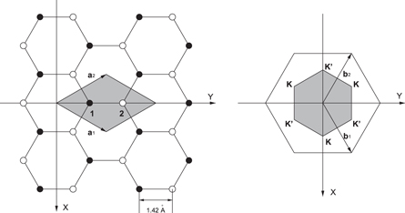
Figure 1. Graphene and its reciprocal lattice. Left: a1 and a2 a1 and a2are the lattice vectors. There are two carbon atoms (1 and 2) in one unit cell (shaded area). Right: the reciprocal lattice of graphene is defined by b1 and b2. The first Brillouin zone is shown as shaded hexagonal [38].
Download figure:
Standard image High-resolution imageOf particular importance for the electron dynamics in graphene are the two points K and K' at the corners of the graphene Brillouin zone (figure 1). These are:
 which are known as Dirac points.
A carbon atom has 6 electrons. Two electrons are in 1S2 shell. Four are in 2S2 and 2p2 sub shells. The first two formed filled energy levels. The three of the four electrons of carbon atom 1 form three σ bonds with the three of four electrons of carbon atom 2 in the plane of the graphene sheet. The σ bonds are localized and form filled energy bands and thus they do not contribute to electron conduction.
The fourth electron is in 2pz orbital which oriented normal to the graphene plane. The fourth electron of carbon atom 1 form π bond with the corresponding electron of atom 2. There are two π band energy – one bonding (valence band-filled- π) and another antibonding (conduction band-unfilled- π'). The idea of massless nature of electrons in the conduction band of graphene emanate from the energy dispersion relations calculated on the basis of tight binding approximation and it is given as follows. Let us call the two 2pz orbitals of the fourth electron in carbon atoms 1 and 2 as Φ1and Φ2respectively [each of which is normalized and Φ1and Φ2 are orthogonal]. The total wave function of the two electrons can be given as (with linear combination of atomic orbitals)

b1 and b2 are the overlapping constants and satisfy the condition

In the graphene lattice the net wave function must follow the periodicity of the lattice R as given by Block wave function:

Considering a single electron to be described by wave function  and its motion is governed by the Hamiltonian H, which is given by the potential of all the carbon atoms as

The wave function  satisfies the Schrodinger equation:

The Hamiltonian  can be written as:

where

And

To get the energy eigenvalues of equation (6) we project it on Φ1 and Φ2 and the two equations

To evaluate equation (10), we consider only nearest neighbor products considering only R = 0, a1 and a2 in equation (4). Then


In equation (10)

To evaluate LHS of equation (11) we note that
 and
and  satisfy,

 is the energy of the
  electron of atom i. Obviously
  We set these equal energies to be zero.
Then

and

where

and 

Using equations (14)–(16), (11a) and (11b), equation (10) becomes, upon neglect of  which is quite small,

β describes the variation of energy of the  atomic orbital induced by electrons of all other carbon atoms in the graphene plane. It corresponds to a small rigid shift of the energy band. It is Reich et al. (2002) that 0.02
 [40]. As an approximation β can be neglected. Equation (17) is further simplified if we exploit the fact that γ0 is small. Then one gets by solving

where ky and kx are the y and x component of the wave vector k in graphene plane. The ± sign refers to upper (π*) band and lower (π) band respectively. On neglect of β the energy dispersion is symmetric around zero energy in k-space. The dispersion close to one of the Dirac points (at the K and K' points in the Brillouin zone, figure 1) using

where  = arc tan
  and
and 
If we neglect the  term then from (18)

Equation (19) gives in the first order approximation, energy of electrons in graphene as proportional to absolute value of momentum.  defines absolute value of momentum relative to the Dirac point. This reminds us of energy dispersion relation for massless relativistic particles (photons, neutrinos etc) that comes from Einstein's relation
with analogy that  being the maximum electron velocity in graphene, replaces c. Even though the first approximation equation (19) gives massless (energy proportional to momentum) nature of electrons in graphene, a cyclotron mass can be attributed to it from the following consideration: within semiclassical approximation the cyclotron mass is given by [Ashcroft and Marmin (1976) [1]]

where 
Using equations (20) and (19) then one gets,

Equation (21) clearly says that

The cyclotron mass determined for electrons in graphene is shown theoretically and found to depend on carrier concentration. It varies from very close to  for low concentration to about
  (rest mass of electron) for carrier concentration, n of about
  [39, 41].
The equation (22) thus shows clearly that  and
and  are related and definitely not two independent quantities as treated in the recent formula for thermionic emission current density derived by Liang and Ang [10].
Equations (21) and (22) become somewhat complicated if one takes into account the second order term in equation (18) that gives the dependence of energy on  This term reminds us that graphene electron is not truly massless, as conjectured from equation (19) and neither it is relativistic in the true sense of term (velocity ∼ 0.1 c or higher). Energy proportional to
  reminds some form of mass attribution to electrons in graphene. Yoon et al. [37] measured kinetic inductance of electrons at microwave frequencies. From such measurements they extracted dynamical electron mass to be in the range
  to
to  Thus, it is not correct to assume electrons to behave completely massless [as per equation (19)] for thermionic emission, as has been done in the treatment of thermionic emission from graphene by Liang and Ang [10]. If we do, the question is how do the electrons acquire mass when ejected out of graphene? It is not possible to answer that by the theory of Liang and Ang. Moreover, the theory has many faults as mentioned earlier [36]. Using equation (19) the density of states, one can easily see that
  becomes proportional to the energy E. This was used in the Liang and Ang model. When we take equation (18) the
  becomes a complicated function of energy E. The derivation of thermionic current density
  relation becomes complicated. Further complication arises from the fact that for thermionic emission the electron must have a component of momentum, kz normal to the graphene plane in addition to components of q in the x-y plane of graphene. A proper model must take the energy quantization along z into account in addition to E(q). Then preliminary investigation shows that it is difficult to get a close form of expression for
For proper performance evaluation of thermionic energy converter with graphene complicated J versus T relation is not helpful and one needs a close form expression.
Based on above discussions, for proper performance evaluation of thermionic energy converter with graphene, in this paper, we have sought an alternative approach to derive the correct  relation that can apply to both graphene and carbon nanotube. In this new approach we have considered the temperature dependence of the Fermi energy
  work function W, along with thermal expansion of materials. We have assumed three-dimensional density of states. During thermionic emission from the surface of monolayer graphene, electron motion cannot be considered as being restricted in two-dimensional plane of graphene (as in the case of electrical current conduction in the plane of graphene or along the length of a CNT) because, for emission perpendicular to the graphene surface, electrons must have in-plane motion as well and thus thermionic emission involves three-dimensional motion of electrons with three components of the wave vector. With wave vectors only along the graphene plane it is not possible to treat or model the thermionic emission perpendicular to the graphene plane. The thermionic electrons (from the graphene surface) will have wave vector components along the direction of emission
  as well as in plane
  The emitted electrons leave vacant energy states within graphene after emission. When the electrons are returned to the emitter via the lead current from the collector (anode) [the anode and emitter are electrically connected] they need to be redistributed to fill those vacant energy states again. This involves an in-plane motion of electron within graphene (emitter) and as a result such electrons must have also wave vector components within the plane of graphene
  Thus, for thermionic emission of electrons even from a monolayer graphene the wave vectors of electrons have three finite components
  of the wave vector and the three-dimensional model for thermionic emission should be valid even for graphene, a two-dimensional material. It is only for thermionic emission from the graphene edges a two -dimensional model would be appropriate but the net current is too insignificant for it to have any practical application. For thermionic emission from the cylindrical surface of a hot CNT the electrons are also expected to have finite non-zero
  components of the wave vectors and hence a three-dimensional density of states should be applicable also for thermionic emission from CNT.
For thermionic emission out of graphene plane electrons must have z-component of momentum. How is this possible in an ideal 2D monolayer graphene? The dispersion relation discussed above (equation (18)) contains in plane wave vector k, that has both  components,
  but not z (normal to the plane) component. A graphene surface from which thermionic emission generally takes place is macroscopic (usually the area is more than 1 cm × 1 cm) and not nanoscopic. Therefore, electron, in all practical reality, follow Bloch wave function guided by periodicity in the plane of graphene and hence these momentum components assume practically continuous values (not discrete). However, for the z-component of motion as the electron is quantum-confined in z-direction (one atom layer in graphene), a z-component of momentum
  can arise (even from uncertainty principle). This z-momentum is intrinsic in the sense that it is there even at 0 K. It does not cause electron emission. There are discrete excited energy levels higher than
  and Fermi energy,
  by definition is the highest occupied energy level at 0 K. At finite temperature electrons start occupying levels higher than EF, the general consensus for thermionic emission along z-direction is that,
  It is an open question how electron in 2D graphene acquire this z-component of momentum and some of the possible ways this can happen are discussed in the appendix B.
Using the three-dimensional density of states and considering thermal expansion, we have obtained an equation W(T) containing terms up to fifth power of T and a final equation for  using the W(T). It provides an excellent fit between our theory and the experimental data of J versus T for both graphene and carbon nanotube. The fits are seen to be far better than those of any existing model. From the best fit of experimental data, we have estimated the variation of
  and W(T) within the given temperature range of the data for both graphene and CNT. Using the new model, we have estimated the effective thermionic mass of electron in graphene for the first time and found to be in excellent agreement with the measurements of dynamic electron mass in literature. The estimated work function at 300 K is also in good agreement with experimental values. These indicate the success of our model. Other existing models fail to determine the effective thermionic mass of electrons from
  data of graphene. After making detailed comparison of the existing models of thermionic emission we find that the new model explains not only the
  data for graphene and CNT but also experimental values of some important physical parameters. The justification for three-dimensional model of thermionic emission for graphene can be understood from the discussion in appendix A and the following.
During thermionic emission from monolayer graphene, electron motion cannot be considered as a restricted two dimensional motion (as in the case of electrical current conduction in the plane of graphene) because, for emission perpendicular to the graphene surface, electrons must have motion in plane as well and thus thermionic emission involves three dimensional motion of electrons with three components of the wave vector and hence it is not surprising that a good three dimensional model with three dimensional density of states as presented here, could excellently fit the thermionic emission from graphene as seen in the results described below. Even in the theory of Liang and Ang [2, 10] which is claimed to be a two- dimensional model, wave vectors both in graphene plane and perpendicular to the plane have been considered. With wave vectors only in the graphene plane it is not possible to treat or model the thermionic emission perpendicular to the graphene plane. The thermionic emission of electrons from the cylindrical surface of a single or multi-walled carbon nanotube must also involve three components of electron wave vector.
Thus, a three-dimensional model of thermionic emission as presented in this work should be valid for graphene and carbon-nanotube. The agreement with experiments as mentioned below for these materials support the model presented in this work.
4. Modification of Richardson-Dushman equation for nano materials
4.1. Variation of work function (W) of a metal with temperature
For nano-materials both the surface density and volume density of free electrons are far less than those in metals and accordingly the Fermi energy is expected to be much less. Its temperature dependence is expected to have greater influence on W than for metals. The relation of W with T depends primarily on the change of  with T. To work out this change we rely on the fact that the total number of electrons
  in a given piece of metal at
  is the same at
  (It is assumed that during thermionic emission in a TEC, electrons will be replaced at the emitter through load current). Now at
  and the Fermi function
Using the concept of density of states  the total number, N of free electrons in the metal are given by: Temperature 0 K,

Finite temperature T,


f(E) is the well-known Fermi-function. (EF(T)) in equation (25) is called chemical potential in many books. We call it temperature dependent Fermi energy level. Considering thermal expansion of the metal,

where α is linear thermal expansion coefficient. Thermionic emission takes place at high temperature  The work function
  is defined as:

where  is the vacuum level.
  is dependent on temperature. Change of
  with T will change the work function with T and this in turn will affect the thermionic emission current density from that given by RD Equation. This is going to play a special role in nano-materials where
  is low at ambient temperature. Our primary objective now is to obtain
  and hence
  as a function of T from the equations (23)–(27) to (35). The 2nd objective is to see how this affects the RD equation (1) and how the modified RD equation fits the experimental results of graphene.
Since  as discussed above, from equations (23) to (26)

Using the expressions for and
and  equation (27) becomes
The LHS of equation (29) is independent of T while the RHS is dependent on T. Solution of this equation (29) for EF as a function of T is a non-trivial problem. There are two ways it can be accomplished as described below:
4.2. Method 1
Expanding the RHS of equation (29) we obtain equations (30)–(33)

Equation (30) after rearrangements becomes

To obtain  as a function of
  and T, we put
 as a first approximation in the RHS of
Equation (31) and we get equation (32)

Using equation (27) we then obtain  is the work function of the material at

4.3. Second method
The second method of obtaining EF as a function of T for a given EF0 involves numerical integration of the RHS of equation (29) using the value of α for the material. To obtain EF at a value of T for a given value of EF0 we have carried out the numerical integration (equation (29)) using,  and the upper limit of the RHS as
  Then for a given
  and T, we find the value of EF that gives close agreement between the LHS and RHS of equation (29) such that the absolute value of the difference between the two lies within
  of the value of the LHS. By changing T we get another value of EF for the same EF0. Thus one can obtain EF as a function of T for a given EF0. Using these
  one can obtain the changes in work function relative to its value at absolute zero, W0. These in turn can be used to obtain
  for graphene for a given value of
  and W0 using the equation (34).

By finding the best fit between the experimental values of J versus T curve for graphene and carbon nanotube one then can obtain the values of W0,  for the materials. It can be seen from computations that the changes in
  i.e.,
i.e.,  increases as
  decreases. This second approach though ideal for nano material in this model, is quite time consuming to generate the
  curves to find the best fit with experimental values.
In equation (33) W0 corresponds to  The numerical coefficients for successive terms after the fourth power of T in equation (33) get smaller and smaller than unity. Moreover, the term
 decreases faster for
  with temperature T such that
  Then terms up to the fourth power of T are sufficient in equation (33). We have verified by actual numerical computation of the equation (29) that
  calculated from equation (32) is within 0.3% of the value obtained by actual numerical computation when EF0 is up to
  and temperature range 300–2500 K. For nano materials like graphene and CNT operating at temperatures less than
  equation (32) or equation (33) is thus sufficient but at temperatures greater than
  sixth or higher power terms would be necessary.
5. New modified Richardson-Dushman equation
As explained earlier, thermionic emission even from graphene (2D) and carbon nanotube (1D) involves electron motions with three finite components of wave vectors. Hence a three-dimensional model of thermionic emission current density should be applicable for both graphene and carbon nanotube. Considering the corresponding thermal expansion coefficient, and using equation (33), the modified Richardson-Dushman Equation (MRDE) for thermoelectron current density (emitted along z direction) is given by:

Where W(T) is given by equation (33). Equation (35a) gives us new thermionic emission equation that should be applied for materials like graphene, carbon nanotubes which have low EF0 and for temperatures less than  For 2D graphene,
  and for 1D CNT,
  in equation (35b) where, it can be easily seen that the effective RD constant is given by

and

The  is related to the free electron concentration by the following equation:

6. Results and Discussions
6.1. Application of modified Richardson-Dushman equation to thermoelectron emission from graphene
In this study, we investigated if the MRDE can be applied to thermoelectron emission from graphene which has exhibited metallic properties [42–44]. Experimental data of J for a mono atomic layer of suspended graphene has been extracted from figure 9(a) of [2]. Using equation (35) and the experimental value of thermal expansion co-efficient  [45, 46] and different values of W0 and
  each step of 0.001, we have examined how the equation fits the experimental values of J versus T for monolayer suspended graphene2 in the temperature range
  We have used visual eye best fitting along with minimum value of
  to ascertain the best fit values of W0 and EF0. The various fits are shown in figures 2 and 3. To obtain the best fit from apparent many good fit (figure 2) we also rely on the value of S (tables 1 and 2). The values of the parameters
  that give the minimum value of S for the experimental data are accepted as the correct value for monolayer graphene. Figure 3 shows the shift from best fit with change of the values of
  in MRDE model. We see that the minimum value of
  is obtained for
  and
and  and the fit is excellent. For other values of W0 and
  we can easily see from figures 2 and 3, that the fit is not as good as that for
  and
and  and the value of S (tables 1 and 2) is significantly higher than the minimum value of
  in the entire temperature range
  By giving a wide variation in the work function of graphene we have examined in detail how the RD law fits (figure 2) the experimental data of
  of graphene in the above temperature range. The best RD law fit is shown in figure 2 for
  This gives the value of
  =
=  (table 2) nearly three times the best fit value as obtained above with MRD. For other values of W the RD law the fit is much worse (tables 1 and 2). By comparing the best MRD law fit (figure 2) with the best RD law fit (figure 2), we can visually also see that the fit is better with MRD law than with RD law. This is reflected in the S values also (tables 1 and 2). This shows the usefulness of our equation (35) for thermoelectron emission current density J. Using equation (35) and the values of W0 and EF0 corresponding to the best fit [figures 2 and 3] of the thermionic data we find that the work function of monolayer graphene increases from
  at
at  to
to  at
at  (figure 4). Surprisingly, like that in CNT, the work function (4.72 eV) corresponding to the best RD law fit of
  data of graphene falls within this range. For nanomaterials
  is quite small compared to metals and our equations (33) and (34) should be used to model
  and thermoelectron emission current density J from nanomaterials. The equations should be used for performance evaluation of TEC using graphene, carbon nanotubes etc as emitter and collector.

Figure 2. Comparison of best fit of J versus T data of monolayer graphene in MRDE model and RD model for different work functions.
Download figure:
Standard image High-resolution image
Figure 3. Influence of  on the best fit of J versus T data of graphene in MRDE model.
Download figure:
Standard image High-resolution imageTable 1.
Values of S for different values of W0 and  in MRDE model of Graphene.
| MRDE GRAPHENE | RD GRAPHENE | |||
|---|---|---|---|---|

|

|
S = 
|

|
S = 
|
| 4.592 | 0.203 | 0.000 171 | 4.592 | 0.531 |
| 4.71 | 0.0020 | |||
| 4.72 | 0.000 553 | |||
| 4.73 | 0.001 70 | |||
| 4.74 | 0.0053 | |||
| 4.68 | 0.0285 | |||
| 4.77 | 0.0245 |
Table 2. Comparison of S for three different models of Graphene: MRDE, RD and Liang and Ang model.
| MRDE GRAPHENE | RD | Liang and Ang | ||||||
|---|---|---|---|---|---|---|---|---|

|

|
S = 
|

|
S = 
|

|
 
|

|
S = 
|
| 4.592 | 0.190 | 0.003 71 | 4.592 | 0.531 | 4.592 | 0.190 | 2.49E6 | 0.1911 |
| 4.592 | 0.210 | 0.000 941 | 4.514 | 2.49 | 4.592 | 0.201 | 2.49E6 | 0.1818 |
| 4.592 | 0.203 | 0.000 171 | 4.72 | 0.000 553 | 4.592 | 0.21 | 2.49E6 | 0.1765 |
| 4.514 | 0.083 | 2.49E6 | 0.2101 | |||||
| 4.514 | 0.083 | 1E6 | 0.0056 |

Figure 4. Temperature variation of work function with temperature for graphene. The middle line corresponds to values of W0 and EF0 for the best fit of J versus T data in graphene.
Download figure:
Standard image High-resolution imageThere are various reports on work function of graphene. Song et al. and Seo et al. [47, 48] claimed to have carried out accurate determination of work function of graphene through a detailed analysis of the capacitance-voltage characteristics of a metal–graphene-oxide-semiconductor (MGOS) capacitor structure. They found a value  for the work function of graphene. Lee et al. [49] measured by scanning kelvin probe microscopy the unbiased work function of graphene to be
  and found that it is influenced by electric field due to bias gate. In our model, the work function of graphene increases with temperature. At
  it is
it is  It is to be noted that the thermionic emission data that has been fitted with our MRD model correspond to that of monolayer suspended graphene of Liang and Ang. We can assume the layer to be pure, i.e., without contamination. The experimentally measured value of pristine graphene is
  [50]. Thus, we see that our estimate of work function of single layer graphene is in close agreement with the experimental values of work function of graphene reported in literature. Our model offers very accurate determination of work function if the thermionic data can be very accurate. To our knowledge, there is no experimental data on temperature dependent measurement of work function of pure monolayer graphene to confirm our theoretical prediction of increase of work function with temperature. Such data could have lent additional credence to the model.
6.2. Thermionic emission from carbon nanotube
After the initial success of MRDE model on thermionic emission from graphene (section 6.1), we apply equation (35a) the modified Richardson-Dushman equation (MRDE) to thermionic emission from CNT. For nanomaterials, because of low density of free electrons compared to metals, Fermi energy (equation (36)) is much lower than that of metals. As a result, the equation (35) should be applicable to nano-materials in its entirety. For metals which has  ∼ 10 eV, it can be shown that equation (35a) essentially reverts back to RD law with effective thermionic constant given by equation (35c).
We rely on the data kindly supplied to us by Wei [11]. Wei et al. [11] performed very careful and delicate studies on individual hot CNTs where simultaneous measurements of J and T have been performed. To simulate the J versus T curve using equation (35) and to study the best fit of the experimental data, we used the value of thermal expansion co-efficient  as obtained by Deng et al. [46] for both single and double walled CNT. We have given systematic wide range of variation by
  to both W0 and EF0. W0 and EF0 are the only two parameters which are varied to obtain the best fit in this paper. Figure 5 shows the theoretical fit (solid line) with experimental data (dots) using equation (35) with
  and
and  The fitting seems good visually. The value of
  for this fit. It gives the lowest value of S as seen by us with wide range of variation of W0 and
  (table 4). The lower the value of S the better is expected to be the overall fitting. Figure 5 also shows the fit with values of W0 and EF0 slightly different from those of the best fit values. We see that as S changes with values of W0 and EF0 [table 4] so does the visual fit of the theoretical curve with the experimental data (figure 5) Thus, with MRDE, figure 5 gives the best fit with value of
  (N = number of the data points) well within the mean experimental error [11]. The variation of work function with temperature for the best fit values of W0 and EF0 and some other values are shown in figure 6 for CNT. The work function increases at an average rate of
  for CNT. One very interesting result that emerges from the fitting with this new model is the best value of
  found for CNT (figure 5). Anantram and Leonard [51] reported that electrons in the crossing sub-bands have a large velocity of
  at the Fermi energy of CNT. If we assume that this is the Fermi velocity than the Fermi energy turns out to be
  which is surprisingly in close agreement with the value
  obtained from the fitting. Apart from good fitting of
  data for CNT, this agreement lends additional credence to the validity of our model for CNT.

Figure 5. Sensitivity of different parameters in MRDE model for fitting J versus T data in CNT.
Download figure:
Standard image High-resolution imageTable 3. Comparison of S for CNT with MRDE and RD models.
| MRDE CNT | RD CNT | |||
|---|---|---|---|---|

|

|
S = 
|

|
S = 
|
| 3.67 | 1.87 | 9870 | 3.67 | 4118 700 |
| 3.69 | 3006 500 | |||
| 3.87 | 324 970 | |||
| 3.91 | 23 366 | |||
| 3.93 | 81 022 |

Figure 6. Temperature variation of work function with temperature for CNT. The middle line corresponds to values of W0 and EF0 for the best fit of J versus T data in CNT.
Download figure:
Standard image High-resolution imageWe next study the comparison of our MRD model with RD law. In RD law, the work function W is temperature independent. To study the fit of the  experimental data with the values obtained by using RD law, we give a systematic variation of W, the work function of CNT, from 3.88 to 3.93 by
  We find that the best fit (figure 7) with RD law is obtained at
  for which the value of
  The RD law fit gets worse (figure 7), with high values of S (table 4) when W is changed by more than 0.01 on either side of
  Now comparing the best MRD fit (figures 7 and 5) of
  experimental values of CNT with the best RD law fit (figure 7), obviously the MRD law gives better fit in terms of both lowest value of S (tables 3 and 4) and the visual eye fitting (figure 7). Thus, MRD is superior to the RD law for CNT. For the best MRDE law in table (4), the W varies from
  to
to  (figure 6) and surprisingly the work function (
 ) for the best RD law fit figure (7) is closed to these values.
Table 4. Comparison of S for CNT for different values of W0 and EF0 in MRDE model.
| MRDE CNT | ||
|---|---|---|

|

|
S = 
|
| 3.67 | 1.87 | 9870 |
| 3.69 | 1.87 | 63 471 |
| 3.67 | 1.89 | 10 360 |
| 3.69 | 1.89 | 75 407 |
| 3.67 | 1.85 | 10 930 |
| 3.69 | 1.85 | 52 633 |
6.3. Application of Liang and Ang's theory to thermionic emissions from graphene
Liang and Ang [2] developed a theory of thermionic emission from graphene based on massless Dirac electrons in graphene. They had seen good agreement with their theory for graphene.
The emission current density J in that theory is shown [2] to be given by


Figure 7. Comparison of best fit of J versus T data of CNT in MRDE model and RD model for different work functions.
Download figure:
Standard image High-resolution imageLiang and Ang [2] used equation (37) and obtained their best fit of the experimental data of J versus T on monolayer suspended graphene for 
 and
and  For these values we obtain S =
 which is nearly 20 times the values of S obtained for the best fit by MRDE model. It should be seen that ϕ − EF should be considered as a single variable in equation (37), instead of two independent variables ϕ and EF, since it is not possible to relate EF and VF in the above equation. We have explained this situation in section 3.1. The lower the value of S the better is the fit expected. The Fermi velocity,
  of electrons in graphene are measured [52] to lie between
  and
and  depending on the substrate in contact and the environment surrounding the graphene. For suspended graphene VF is measured to be as high as
  It is found to be inversely proportional to the dielectric constant of the substrate in contact. For monolayer graphene
  [52] is more appropriate than the value
  used by Liang and Ang. Now if we use the exact value of
  as obtained experimentally for monolayer graphene, the value of S becomes
  which is 1254 times the value obtained with MRD. If we use
  then S is
  which is 676 times the minimum value of S obtained with our model. Thus, our MRD equation fits the thermionic emission current density in graphene far better than that of Liang and Ang's theory and that by RD law. Figure 8 shows the comparison of the three models (MRDE, RD and Liang and Ang) in one plot.

Figure 8. Comparison of Liang and Ang model for different parameters with MRDE model best fit of J versus T data of monolayer graphene.
Download figure:
Standard image High-resolution image
In the light of discovery of finite dynamic mass or effective mass of electron in graphene, the theory raises questions as mentioned earlier. However, we have examined to see if the theory can fit the experimental data in graphene better than our MRD equation. As explained earlier in section 3.1. some form of mass (though smaller than free electron mass) needs to be attributed to electrons in graphene.
6.4. Temperature dependence of work functions for graphene and CNT
We have included the plot of temperature variation of work function for graphene and CNT. We have shown in figure 6 the variation of work functions for slightly different values of EF0. The graphs show the average  for graphene is
  and
and  for CNT.
We do not have experimental data for temperature coefficient,  of work function of all metals. Moreover, all metals are not expected to behave in the same way. We refer to the work of Ibragimov and Korol'kov (2001) [53]. From there we see that experimental μ for Ga, In, Sn, Bi, Tl and Pb are (in units of
  ): 23.1, 25.3, 23.4, 13, 30 and 28 respectively. Thus, we see that
  for these metals is smaller than that of graphene and CNT by a factor 7.8 and 6.2 respectively. Thus even though the temperature dependence of J from metals can be roughly described by
  for graphene and CNT, temperature dependence of J should be described by equation (35a).
7. Conclusion
We have considered first the existing theory of electron energy dispersion in 2D monolayer graphene to reconsider the massless nature of electron in graphene and the relations between Fermi velocity and Fermi energy of electrons in graphene as these are important for any new models on thermionic emission from graphene. We then consider various existing models for thermionic emission from nano materials. We find that there exists none that truly explains all the features of thermionic emission from such materials. We then give justifications that a three-dimensional model should be applicable for thermionic emission from nano materials such as CNT and graphene. We have presented briefly the physics of graphene as existing already in literature. We see that Fermi energy and Fermi velocity are not two independent quantities but rather related. Moreover, we see that the electrons in graphene are not truly massless as often is conjectured. The presence of terms with both  and
and  in energy [equation (19)] makes the expression for density of states complicated for a thermionic emission current density (J) versus T relation to be smoothly applicable for performance evaluation of a graphene based TEC. Further complication is added when the terms γ0 and β are included and not neglected, as before, in the energy dispersion relation. Moreover, as explained earlier, the graphene electron mass cannot be said to be truly massless when these terms are considered (as ideally it should be) in the energy dispersion relation. The observed finite dynamic mass supports this view.
In the light of the above, thus, for proper performance evaluation of TEC with graphene we have considered a simple model of temperature variation of work function of metals considering thermal expansion and temperature variation of Fermi energy (chemical potential) to obtain theoretical expression for temperature dependent work function,  [equation (35b)]. We have modified Richardson-Dushman Equation (MRDE) [equation (34)] using the
  The new equations (35a), (35b) are different from that of RD equation. In nano-materials like graphene and carbon nanotube the electron density and consequently the Fermi energy, EF0 is much lower than that of metals. Thus, it should be applicable for nano-materials. We have seen that our new thermionic emission current density equation fits excellently well the experimental data for monolayer graphene (without the substrate effect) and much better than any existing models. We have determined this by studying the variation of S =
  for wide range of variables for the different existing models and obtaining the minimum values of S with different models and comparing the minimum values and using the visual eye fit which agrees completely with minimum S as expected. Moreover, the advantage of the new model unlike any other model, is that it provides unique and accurate method of determination of EF over the entire temperature range starting from 0 K, which RD law and other models cannot provide. The work function of suspended monolayer graphene is seen to change from
  to
to  as temperature changes from
  to
to  and EF from 0.203 to
  in the temperature range 0 to
  This change in work function with temperature influences the thermionic emission in accordance with equation (35b) in graphene, a fact that has not been considered before in literature. The model fits the
  data for CNT very well and better than RD law. The values of work function determined with our model for graphene also agrees very well experimental value [50]. The Fermi energy determined from the model for CNT agrees fairly well with independent estimate of Fermi velocity. These excellent agreements with independent experimental results show strong support for the model of thermionic emission current density from graphene and CNT presented in this work.
The model is expected to help accurate simulation of performance of thermionic energy converter with graphene or carbon nanotube. Our models lend an estimate of temperature dependent Fermi energy of graphene from the  data of thermionic emission. We have shown that the MRDE model fits the
  data of graphene better than the Liang and Ang model.
Nanomaterials have been proposed to be good candidates for thermionic energy converters, specially solar energy. Our above equation should be used to simulate accurately the performance of such TEC, instead of ordinary RD law. Moreover, for electric field emission of electrons from nano materials at finite temperature, the temperature dependence of work function should play an important role and for modification of Fowler- Nordheim law for nano material, the temperature dependence of work function as mentioned above should be important [54].
Acknowledgments
The authors gratefully acknowledge the facilities provided by the Covenant University to carry out the reported research works. The authors thankfully acknowledge the experimental data for carbon nanotubes and graphene provided by Xianlong Wei of Peking University, and Professor Jiang Kaili of TSinghua University .
Appendix A
TEC-Thermionic energy converter; CNT-Carbon Nano-Tube; RD-Richardson-Dushman; MGOS-Metal Graphene-Oxide-Semiconductor; MRD-Modified Richardson-Dushman
Appendix B
There can't be any denying to the simple fact that for thermionic emission from the graphene flat plane there must be a component of electron momentum perpendicular to the graphene plane. How the electron acquires this momentum is not the objective of this paper. However, we have narrated below a few possible mechanisms for this.
In thermionic emission and in absence of an external electric field in the plane of graphene, the electrons receive momentum as a result of collision with phonons mostly. As electrons are emitted it cools the graphene, because electrons are taking the energy from the lattice, unless energy is supplied in the form of heat. To maintain it at the temperature of the emissions, thermal energy from external source enter the lattice through collision. If the thermal source is in the form of heat radiation (without any hot lattice in contact with the graphene) then the thermal photons, which in general have all the three momentum components can transfer the z-component momentum to the electrons of graphene during collision. It is to be noted that in a good heat conductor it is the electrons that conduct heat more than the lattice and also the electrons contribute more than the lattice in overall thermalization (to achieve a constant temperature throughout). If the thermal source is in the form of hot substrate directly in contact with graphene, then the phonons of the substrate lattice which have all the three components of momentum impact the electrons of graphene which then can get the z-component of the momentum through collision with such phonons. The electron emission takes place only when the z-component of the momentum, Pz satisfies the relation  .
.
W = work function. The lattice phonons in graphene can also have three components of momentum because the atoms in graphene can vibrate in all three directions (x, y, z) directions. The vibrations in the z-directions could be in a transverse wave form while the vibrations in x-y plane are longitudinal. If the free electrons are impacted by phonons which have momentum components in x, y, z directions, the electrons can receive the z-component of momentum from conservation principle that hold during collision.
In the above scenarios one may argue that only high energy spectrum of thermal photons or lattice phonons would be able to give enough momentum to electron for emission. In such case the efficiency of thermionic emission would be very low. However, multiphotonic or multi-phonon collisions with electrons will be needed for the required momentum transfer.
We feel that at a given temperature, the conservation of momentum must hold for electron motions in the plane of graphene (in absence of any external field), if we neglect the edge thermionic emissions. The huge uncertainty in z-component of electron momentum which is present in graphene even at 0 K does not take part (either positively or negatively) in thermionic emission. If it did, the emission would have been seen at 0 K even. Emission along z-direction takes place at elevated temperature and as explained above it is possible only when the phonons or photons transfer to electrons the z-component of momentum sufficient for emission to take place. In our opinion there can't be any cross momentum transfer- i.e., the in-plane components of momentum being converted to z-component of momentum. This is not possible. This latter part, if at all would be possible, would require a new physics.