Implementation of continuous-variable quantum key distribution with discrete modulation

Quantum key distribution (QKD) offers secure communication based on the fundamental laws of quantum physics [1]. In contrast to public key cryptography that is currently in wide-spread use and whose security relies on the computational difficulty of solving a mathematical problem [2], the security of QKD can be guaranteed even if an eavesdropper has an infinite computational power [3]. QKD enables two parties, usually called Alice and Bob, to share a secret key that is unknown to third parties by sending quantum states from Alice to Bob [4].

Continuous-variable (CV) QKD is different from the standard QKD system in the method for detecting weak optical signals [5–11]. This feature gives an advantage to CV-QKD in terms of practical implementation. In the standard QKD system, weak light is detected by a single photon detector that measures the particle nature of light: the measured observable has a discrete spectrum [4]. The detector is usually custom built for QKD, requires cooling, and expensive, and it is sensitive to stray light. On the other hand, in the CV-QKD weak light is detected by a homodyne detector that measures wave nature of light: the measured observable has continuous spectrum. A homodyne receiver is commercially available, works at room temperature, is low cost and small and insensitive to stray light because the local oscillator (LO) itself works as a spectral, temporal and spatial mode filter. Since both CV-QKD and coherent optical communication exploit devices which operate on the same principle, we may be able to realise a secure and safe communication infrastructure that can offer diverse functions ranging from unconditionally secure communications to high-speed and high-security data transmission in a unified way, and seamlessly integrate them into coherent optical communication systems [12].

However, in terms of security analysis, the security proof of CV-QKD is relatively difficult compared with the discrete variable (DV) QKD that uses a single photon detector. In the case of DV-QKD, one can intuitively understand its safety as follows: if Alice sends only a single photon and Bob detects the photon, an eavesdropper cannot read the information encoded on the photon because a single photon cannot be divided. Even when Alice may send multiple photons, using the so-called tagging idea which was proposed by Gottesman, Lo, Lütkenhaus and Preskill [13], it is possible to use the idea of single photon case to the practical case using weak coherent pulses. On the other hand, in the case of CV-QKD, Bob measures the amplitude of the electromagnetic field, and the amplitude might be divided by an eavesdropper. Indeed, it was pointed out that CV-QKD protocols require that the transmission of the optical line between Alice and Bob is larger than 50% [14], because if the transmission is less than 50%, Eve can obtain higher signal-to-noise ratio than Bob by replacing the lossy channel with her lossless channel and splitting a fraction of the signal with a ratio of larger than 50%. Fortunately, it is known that this apparent 3 dB loss limit can be beaten by using appropriate recipes [15]. One recipe is the post-selection [15, 16]. Post-selection is an intrinsic procedure in DV-QKD: if no photon is detected, the corresponding time slot is discarded. In CV-QKD, Bob can postselect a subset of data by selecting only time slots for which his homodyne detector outputs a high absolute value and the mutual information between Alice and Bob is high. Another recipe is the reverse reconciliation (RR) [6], in which the reconciliation procedure is reversed: Alice's data is corrected to match Bob's data rather than Bob's data being corrected to match Alice's. In this case, Eve has to guess what was received by Bob rather than what was send by Alice, and Alice is advantageous than Eve in guessing Bob's measurement results. Some another recipes such as multidimensional reconciliation [17] and repetition code [18] were propose to improve the performance of CV-QKD. As the bit error rate is crucial when evaluating the security of DV-QKD, an excess noise is crucial in CV-QKD. It is known that if the excess noise of a quantum channel is Gaussian and two times larger than the transmission of the channel, no form of optical communication that uses coherent states and homodyne detection can be secured quantum mechanically since there is a realistic intercept-resend attack [19].

CV-QKD protocols can be classified into two types by the modulation method of coherent states sent by Alice. One is Gaussian-modulation protocol [6, 14] and the other is discrete-modulation protocol [16, 20]. In the former protocol, Alice's state preparation can be formally described in an entanglement based scheme where Alice has CV entanglement [21]. Heid et al pointed out that all collective attacks are unitarily equivalent if the quantum channel can be verified as being symmetric and Gaussian, then secure key rate in the collective attack scenario can be calculated by choosing the entangling cloner attack (see section 3) as an optimal attack including post-selection [22]. Security analysis for the former is more advanced than for the latter, and recently a composable security proof including finite-size setting was reported [23]. Various reconciliation methods for the former protocol have been studied [17, 18, 24, 25]. As for the latter discrete-modulation protocol, it was reported that secure long-distance QKD is possible if the quantum channel can be verified as being linear [20, 26]. The former protocol is more advanced than the latter also in experimental implementation. In 2009, a field test of the former CV-QKD protocol was demonstrated over 9 km fibre with 8 kbit s⁻¹ key generation rate in the SECOQC project [27]. Recently, a long-distance experiment over 100 km was reported by controlling excess noise [9]. In a field implementation of CV-QKD network, computed key rates of 0.25, 2, 6, 10 kbps for 17.52, 15.34, 19.92, 2.08 km link, respectively, were reported using a 500 KHz pulse train [28].

In this paper, we experimentally demonstrate the discrete-modulation (four states) CV-QKD protocol proposed in [5] over a 10 km single mode fibre (SMF) and theoretically evaluate the secure key rate on the assumption that the eavesdropper performs the entangling cloner attack [21, 22]. To our knowledge, this is the first practical implementation of the four-state CV-QKD in which secure keys can be continuously generated by programmed operation. The system is simple, can be built at low cost and operate robustly, thus addresses some of the important challenges toward practical popularisation of QKD [29]. On the theoretical side, we give an algebraic formula for the key rate by using Gramian matrices and show that reverse reconciliation (RR) gives better key rate than direct reconciliation (DR), as shown for CV-QKD protocols with Gaussian modulations [6]. An average photon number of the weak coherent pulse is selected to maximise the secure key rate. On the experimental side, we developed a CV-QKD system that can continuously generate secret key. Key generation rate is 50 kbps when the quantum channel is a 10 km optical fibre. We use a pulsed light source whose wavelength is 1550 nm and repetition rate is 10 MHz. A commercially available balanced receiver is used to realise shot-noise-limited pulsed homodyne detection. We use a non-binary low-density parity check (LDPC) code for error correction [34] and a fast privacy amplification algorithm using the Toeplitz matrix multiplication [35]. A graphical processing unit (GPU) card is used to accelerate the software-based post-processing.

This paper is organised as follows. In section 2, we introduce our CV-QKD protocol and present a set of basic formulas to describe the performance of our protocol under a noisy channel. In section 3, we introduce the entangling cloner attack and calculate the Holevo quantity for DR and RR. Key rates and optimised average photon number are given in section 4. In section 5, we show our experimental implementation and in section 6 we report automated QKD demonstration over 10 km. Section 7 concludes this paper.

The protocol we are going to analyse consists of the following eight steps: (i) Alice sends Bob a quantum state $| S\rangle$, which is randomly chosen out of four coherent states $| \pm \alpha \rangle ,| \pm i\alpha \rangle$ of a given mode. Here, $\alpha \gt 0$. (ii) Bob performs a measurement on the received state with x-basis or p-basis randomly chosen. Here, we defined the quadratures

$$\begin{eqnarray}&&x=\displaystyle \frac{a+{a}^{\dagger }}{2},\qquad p=\displaystyle \frac{a-{a}^{\dagger }}{2i},\end{eqnarray} \tag{ 1 }$$

through the annihilation operator a of the mode A. (iii) Alice and Bob repeat processes (i) and (ii) sufficiently many times. (iv) Alice reveals which basis she used in each process through a classical channel. She also randomly chooses a part of the processes and reveals the state she sent. (v) Bob estimates the parameters of the quantum channel using the data of the processes that Alice revealed her states. Then he selects the data to be used for key generation in accordance with his measurement and the estimated channel parameters. He uses only the processes for which he made a correct choice of the measurement basis. Here, the correct basis refers to the x-basis for $| \pm \alpha \rangle$, whereas the p-basis for $| \pm i\alpha \rangle$. Bob informs Alice which process was selected. In the theoretical analysis, we assume that Bob reveals also the absolute value $| m|$ of his outcome m. (vi) Bob makes a bit string by assigning 0 for the negative m, while 1 for the positive m of selected measurement, respectively. (vii) Alice makes a bit string by assigning 0 for $| -\alpha \rangle ,| -i\alpha \rangle$, whereas 1 for $| \alpha \rangle ,| i\alpha \rangle$. (viii) Alice and Bob share a secure key by applying error correction and privacy amplification to the bit strings obtained. The efficiency of the post-processing could be substantially different whether one chooses DR or RR.

The role of the quadrature x, p is clearly symmetric in this protocol. Without loss of generality, therefore, we may restrict ourselves only to the case of the correct measurements that Alice sends the coherent states $S=\pm \alpha$ and Bob performs the x-basis measurements. Note that the probabilities that $S=\pm \alpha$ is given by $P(\alpha )=P(-\alpha )=1/2$, respectively.

Let us assume that quantum channel is not ideal, but characterised by excess noise ξ and transmission η. The probability density to obtain m conditioned by S is given by [30]

$$\begin{eqnarray}&&P(m| S)=\sqrt{\displaystyle \frac{2}{\pi (1+\xi )}}{e}^{-2\tfrac{{(m-\sqrt{\eta }S)}^{2}}{1+\xi }},\end{eqnarray} \tag{ 2 }$$

when the vacuum noise variance is 1/4. Note that

$$\begin{eqnarray}&&P(m| S)=P(-m| -S).\end{eqnarray} \tag{ 3 }$$

It immediately follows from equation (3) that given the absolute value $| m|$, the protocol can be seen as a binary symmetric channel [31]. To show this, let us define the probability that Alice's 0 goes to Bob's 1. We then find

$$\begin{eqnarray}&&\epsilon := \displaystyle \frac{P(-| m| | \alpha )}{P(m| \alpha )+P(-m| \alpha )}=\displaystyle \frac{P(| m| | -\alpha )}{P(m| -\alpha )+P(-m| -\alpha )}={\left[1+{e}^{8\tfrac{\sqrt{\eta }}{1+\xi }| m| \alpha }\right]}^{-1},\end{eqnarray} \tag{ 4 }$$

which proves the claim, since from the second equality now reads the probability that Alice's 1 goes to Bob's 0. Thus, we may use the Shannon formula and find the mutual information ${I}_{\mathrm{AB}}$ between Alice and Bob as

$$\begin{eqnarray}&&{I}_{\mathrm{AB}}=1-h(\epsilon ),\end{eqnarray} \tag{ 5 }$$

where $h(\epsilon )=-\epsilon {\mathrm{log}}_{2}\epsilon -(1-\epsilon ){\mathrm{log}}_{2}(1-\epsilon )$ is the binary entropy.

An advantage of this four-state CV-QKD protocol is its implementation simplicity. In step (i), Alice performs one of four kinds of phase modulations and in step (ii), Bob performs one of two kinds of phase modulations. Therefore, only a phase modulator for each station is necessary as an experimental device for modulation, and the required random number is 2 bits for Alice and 1 bit for Bob. In the Gaussian-modulated coherent states CV-QKD protocol [6–9], Alice needs also an amplitude modulator and two random real numbers, which are not computable in principle and experimentally she needs random bit strings longer than at least the resolution of the digital-to-analogue converters.

We shall consider the key rate of our protocol against collective attacks assuming that the quantum channel is Gaussian. When the quantum channel is symmetric and Gaussian, all collective attacks are unitarily equivalent [22]. Therefore, in the following we calculate the secret fraction against the entangling cloner attack [21]. Prior to this, we present the details of the entangling cloner attack and evaluate the information accessible by an eavesdropper, say Eve, in this section.

For the entangling cloner attack, Eve prepares an Einstein-Podolsky-Rosen (EPR) state

$$\begin{eqnarray}&&| \mathrm{EPR}\rangle =\sqrt{\displaystyle \frac{2}{\pi }}{\displaystyle \int }_{-\infty }^{\infty }{\displaystyle \int }_{-\infty }^{\infty }{{dx}}_{1}{{dx}}_{2}\ {e}^{-{{Vx}}_{1}^{2}-{x}_{2}^{2}/V}{\left|\displaystyle \frac{{x}_{1}+{x}_{2}}{\sqrt{2}}\right\rangle }_{{E}_{1}}{\left|\displaystyle \frac{{x}_{1}-{x}_{2}}{\sqrt{2}}\right\rangle }_{{E}_{2}}\end{eqnarray} \tag{ 6 }$$

of modes ${E}_{1}$ and ${E}_{2}$. Here ${| x\rangle }_{{E}_{i}}$ represents the eigenstate of a quadrature operator x of the mode ${E}_{i}$ with eigenvalue x. The parameter $V\geqslant 1$ is chosen in such a way that

$$\begin{eqnarray}&&\displaystyle \frac{1}{2}\left(V+\displaystyle \frac{1}{V}\right)=\displaystyle \frac{1-\eta +\xi }{1-\eta }\end{eqnarray} \tag{ 7 }$$

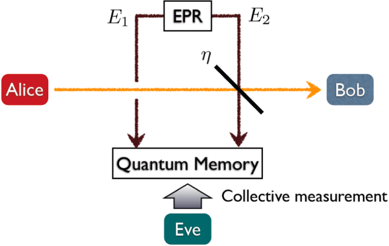
so as to emulate the noisy quantum channel introduced in the previous section. Eve next replaces the noisy quantum channel with a lossless and noiseless quantum channel followed by a beam splitter of transmission η (see figure 1). She then makes interference between the mode A and ${E}_{2}$ by using the beam splitter. After Alice and Bob make a sufficiently long bit sequence, Eve obtains the information of the sequence by performing a collective measurement on the states coming from ${E}_{1}$ and ${E}_{2}$ modes kept in her quantum memory.

Zoom In Zoom Out Reset image size

Let us describe the attack in detail. Since the coherent state $| S\rangle$ can be written as

$$\begin{eqnarray}&&| S\rangle ={\left(\displaystyle \frac{2}{\pi }\right)}^{\tfrac{1}{4}}{\int }_{-\infty }^{\infty }{dx}\,{e}^{-{(x-S)}^{2}}| x\rangle \end{eqnarray} \tag{ 8 }$$

and the beam splitter of transmission η leads to a transformation

$$\begin{eqnarray}&&{| x\rangle }_{A}| {x}_{2}{\rangle }_{{E}_{2}}\to | \sqrt{\eta }x-\sqrt{1-\eta }{x}_{2}{\rangle }_{A}| \sqrt{1-\eta }x+\sqrt{\eta }{x}_{2}{\rangle }_{{E}_{2}},\end{eqnarray} \tag{ 9 }$$

the state after the interference takes the form of

$$\begin{eqnarray}&&{| S\rangle }_{A}| \mathrm{EPR}\rangle \to {\int }_{-\infty }^{\infty }{dm}{| m\rangle }_{A}| \psi (S,m)\rangle ,\end{eqnarray} \tag{ 10 }$$

where

$$\begin{eqnarray}&&| \psi (S,m)\rangle ={\left(\displaystyle \frac{8}{{\pi }^{3}{\eta }^{2}}\right)}^{\tfrac{1}{4}}{\displaystyle \int }_{-\infty }^{\infty }{\displaystyle \int }_{-\infty }^{\infty }{{dx}}_{1}{{dx}}_{2}\,\psi (S,m){\left|\displaystyle \frac{{x}_{1}+{x}_{2}}{\sqrt{2}}\right\rangle }_{{E}_{1}}{\left|\sqrt{\displaystyle \frac{1-\eta }{\eta }}m+\displaystyle \frac{{x}_{1}-{x}_{2}}{\sqrt{2\eta }}\right\rangle }_{{E}_{2}}\end{eqnarray} \tag{ 11 }$$

with

$$\begin{eqnarray}&&\psi (S,m)={e}^{-{\left[\sqrt{\tfrac{1-\eta }{2\eta }}({x}_{1}-{x}_{2})+\displaystyle \frac{m}{\sqrt{\eta }}-S\right]}^{2}-{{Vx}}_{1}^{2}-{x}_{2}^{2}/V}.\end{eqnarray} \tag{ 12 }$$

To obtain this, we have changed the variable x in equation (8) to $m=\sqrt{\eta }x-\sqrt{1-\eta }({x}_{1}-{x}_{2})/\sqrt{2}$. Note that $| \psi (S,m)\rangle$ has the following normalisation:

$$\begin{eqnarray}&&\langle \psi (S,m)| \psi (S,m)\rangle =P(m| S).\end{eqnarray} \tag{ 13 }$$

For later convenience, we introduce

$$\begin{eqnarray}&&| {e}_{{ij}}\rangle ={ \mathcal N }| \psi ({(-1)}^{i}| S| ,{(-1)}^{j}| m| )\rangle ,\end{eqnarray} \tag{ 14 }$$

where i, j = 0, 1 and ${ \mathcal N }$ is a normalisation factor which implicitly depends on $i,j$.

Now, suppose that Bob performs the x-basis measurement to the mode A and find an outcome m. On this situation, Eve has the following two strategies to attack, depending on the reconciliation Alice and Bob adopted: (a) For DR, Eve attacks Alice to estimate her bit. This estimation results in distinguishing

$$\begin{eqnarray}{\rho }_{{\rm{A}}}^{0} & = & (1-\epsilon )| {e}_{00}\rangle \langle {e}_{00}| +\epsilon | {e}_{01}\rangle \langle {e}_{01}| ,\\ {\rho }_{{\rm{A}}}^{1} & = & (1-\epsilon )| {e}_{11}\rangle \langle {e}_{11}| +\epsilon | {e}_{10}\rangle \langle {e}_{10}| .\end{eqnarray} \tag{ 15 }$$

(b) For RR, Eve attacks Bob, aiming at estimate of his bit. By the similar way to DR, this results in distinguishing two density matrices

$$\begin{eqnarray}{\rho }_{{\rm{B}}}^{0} & = & (1-\epsilon )| {e}_{00}\rangle \langle {e}_{00}| +\epsilon | {e}_{10}\rangle \langle {e}_{10}| ,\\ {\rho }_{{\rm{B}}}^{1} & = & (1-\epsilon )| {e}_{11}\rangle \langle {e}_{11}| +\epsilon | {e}_{01}\rangle \langle {e}_{01}| .\end{eqnarray} \tag{ 16 }$$

In both cases, it is known that the information accessible to Eve is bounded from above by the Holevo quantity χ, which is given by

$$\begin{eqnarray}\chi =\left\{\begin{array}{cc}S(\rho )-S({\rho }_{{\rm{A}}}^{0})/2-S({\rho }_{{\rm{A}}}^{1})/2 & \mathrm{for}\ \mathrm{DR},\\ S(\rho )-S({\rho }_{{\rm{B}}}^{0})/2-S({\rho }_{{\rm{B}}}^{1})/2 & \mathrm{for}\ \mathrm{RR},\end{array}\right.\end{eqnarray} \tag{ 17 }$$

where $\rho := ({\rho }_{{\rm{A}}}^{0}+{\rho }_{{\rm{A}}}^{1})/2=({\rho }_{{\rm{B}}}^{0}+{\rho }_{{\rm{B}}}^{1})/2$ and $S(\rho )=-\mathrm{Tr}(\rho {\mathrm{log}}_{2}\rho )$ denotes the von Neumann entropy.

To compute the Holevo quantity χ, we will determine the eigenvalues of all the density matrices appearing in equation (17). Despite all these are infinite dimensional Hermite operators written as a convex combination of projectors not necessarily orthogonal to one another, it is straightforward to find their non-zero eigenvalues by using scaled Gramian matrices, which is defined below.

Given a density matrix $\sigma ={\sum }_{i}{p}_{i}| {\varphi }_{i}\rangle \langle {\varphi }_{i}|$, where $\{{p}_{i}\}$ is a probability distribution, the rescaled Gramian matrix $G=({G}_{{ij}})$ associated with σ is defined by

$$\begin{eqnarray}&&{G}_{{ij}}=\sqrt{{p}_{i}{p}_{j}}\langle {\varphi }_{i}| {\varphi }_{j}\rangle .\end{eqnarray} \tag{ 18 }$$

We then find the following proposition.

Proposition 1. All the non-zero eigenvalues of $\sigma$ are identical to all those of the associated Gramian matrix $G$.

Proof. See [32]. ■

This proposition reduces the calculation of the Holevo quantity to much milder problems: the eigenvalue problems of the Gramian matrices associated with ${\rho }_{{\rm{A}}}^{i},{\rho }_{{\rm{B}}}^{i}$, and ρ. In what follows, we list the Gramian matrices and their eigenvalues. (1) For ${\rho }_{{\rm{A}}}^{i}$, G is independent of i and given by

$$\begin{eqnarray}G=\left(\begin{array}{cc}1-\epsilon & \delta s\\ \delta s & \epsilon \end{array}\right)\end{eqnarray} \tag{ 19 }$$

whose eigenvalues are readily found to be

$$\begin{eqnarray}&&\displaystyle \frac{1}{2}[1\pm \sqrt{1-4{\delta }^{2}(1-{s}^{2})}],\end{eqnarray} \tag{ 20 }$$

where we introduced

$$\begin{eqnarray}s & = & \langle {e}_{00}| {e}_{01}\rangle =\langle {e}_{11}| {e}_{10}\rangle ={e}^{-2\tfrac{\xi (2+\xi )}{1+\xi }{m}^{2}},\\ \delta & = & \sqrt{\epsilon (1-\epsilon )}.\end{eqnarray} \tag{ 21 }$$

Note that, independent of α and η, it holds

$$\begin{eqnarray}&&S({\rho }_{{\rm{A}}}^{0})=S({\rho }_{{\rm{A}}}^{1}).\end{eqnarray} \tag{ 22 }$$

(2) For ${\rho }_{{\rm{B}}}^{i}$, the Gramian matrix is also independent of i and takes the form of

$$\begin{eqnarray}G=\left(\begin{array}{cc}1-\epsilon & \delta t\\ \delta t & \epsilon \end{array}\right),\end{eqnarray} \tag{ 23 }$$

whose eigenvalues are

$$\begin{eqnarray}&&\displaystyle \frac{1}{2}[1\pm \sqrt{1-4{\delta }^{2}(1-{t}^{2})}],\end{eqnarray} \tag{ 24 }$$

where

$$\begin{eqnarray}&&t=\langle {e}_{00}| {e}_{10}\rangle =\langle {e}_{11}| {e}_{01}\rangle ={e}^{-2\tfrac{1+\xi -\eta }{1+\xi }{\alpha }^{2}}.\end{eqnarray} \tag{ 25 }$$

Note also that, independent of m, it holds

$$\begin{eqnarray}&&S({\rho }_{{\rm{B}}}^{0})=S({\rho }_{{\rm{B}}}^{1}).\end{eqnarray} \tag{ 26 }$$

(3) For ρ, we obtain

$$\begin{eqnarray}G=\displaystyle \frac{1}{2}\left(\begin{array}{cccc}1-\epsilon & \delta s & \delta t & (1-\epsilon ){stu}\\ \delta s & \epsilon & \epsilon {st}/u & \delta t\\ \delta t & \epsilon {st}/u & \epsilon & \delta s\\ (1-\epsilon ){stu} & \delta t & \delta s & 1-\epsilon \end{array}\right)\end{eqnarray} \tag{ 27 }$$

with

$$\begin{eqnarray}&&u={e}^{4\tfrac{\xi \sqrt{\eta }}{1+\xi }\alpha | m| }.\end{eqnarray} \tag{ 28 }$$

The eigenvalues of G in equation (27) can be written as

$$\begin{eqnarray}&&\displaystyle \frac{1}{4u}({v}_{+}\pm \sqrt{{v}_{+}^{2}-{w}_{+}}),\quad \displaystyle \frac{1}{4u}({v}_{-}\pm \sqrt{{v}_{-}^{2}+{w}_{-}}),\end{eqnarray} \tag{ 29 }$$

where we defined

$$\begin{eqnarray}{v}_{\pm } & = & u\pm {st}[\epsilon +(1-\epsilon ){u}^{2}],\\ {w}_{\pm } & = & 4{\delta }^{2}u[{st}{(1-u)}^{2}\pm (1-{s}^{2})(1-{t}^{2})u].\end{eqnarray} \tag{ 30 }$$

Plugging equations (22) and (26) into equation (17), we clearly observe that $S({\rho }_{{\rm{A}}}^{i})$ is responsible for the behaviour of ${\chi }_{{\rm{E}}}$ in case of the DR, whereas $S({\rho }_{{\rm{B}}}^{i})$ is responsible for the behaviour of ${\chi }_{{\rm{E}}}$ in case of the RR: the difference between the behaviour of the Holevo quantities for the DR and RR comes from the difference between $S({\rho }_{{\rm{A}}}^{i})$ and $S({\rho }_{{\rm{B}}}^{i})$.

Now we come to the point to evaluate the secret fraction r of the protocol under the entangling cloner attack. Here, the secret fraction r is given by the average of the information difference:

$$\begin{eqnarray}&&r=\displaystyle \sum _{S=\pm \alpha }\int {dm}\,P(m,S){\rm{\Delta }}I,\end{eqnarray} \tag{ 31 }$$

where

$$\begin{eqnarray}&&{\rm{\Delta }}I={I}_{\mathrm{AB}}-\chi .\end{eqnarray} \tag{ 32 }$$

Here, the integral is taken over the region where ${\rm{\Delta }}I\geqslant 0$. This means that we perform a post-selection to the parameter region where the accessible information of Alice and Bob exceeds that of Eve. This corresponds to the selection in step (v). Note that the joint probability density $P(m,S)$ satisfies $P(m,S)=P(m| S)P(S)=P(m| S)/2$, since $P(\pm \alpha )=1/2$. We also note that

$$\begin{eqnarray}&&{\rm{\Delta }}I{| }_{m,S}={\rm{\Delta }}I{| }_{-m,-S},\end{eqnarray} \tag{ 33 }$$

since $\epsilon ,s,t,u$ are symmetric with respect to the conversions $S\to -S$ and $m\to -m$, respectively. By using equations (3) and (33), we can rewrite the secret fraction r as the following simpler form

$$\begin{eqnarray}&&r=\int {dm}\,P(m| \alpha ){\rm{\Delta }}I.\end{eqnarray} \tag{ 34 }$$

Figure 2 shows the optimised secret fractions in the cases of DR and RR, respectively. In the short distance less than 10 km, these two schemes make not so much difference in the secret fraction. In contrast to this, in a longer-distance, RR clearly yields the better secret fraction than DR, as shown in a CV-QKD with Gaussian modulations [22]. Unlike the secret fraction, however, the associated average photon number in DR shows the similar behaviour to that in RR (see figure 3).

Zoom In Zoom Out Reset image size

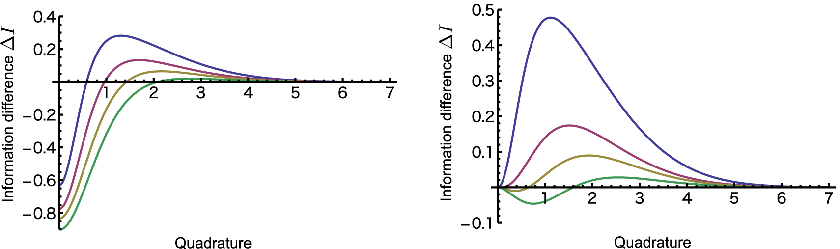
Zoom In Zoom Out Reset image size

The information difference ${\rm{\Delta }}I$ at the optimal case is of interest, since it determines how many measurement outcomes should be chosen by the post-selections. From figure 4, we observe the followings. First, there is at most one non-zero zero point such that ${\rm{\Delta }}I=0$ in both the schemes. Thus, it turns out that the post-selection should be performed over the outcomes whose absolute values are larger than this zero point. Note that this post-selection scheme is exactly the same as that in [5] introduced so as to reduce the bit error rate of sifted keys. Second, RR requires almost no post-selection in the short distance less than about 20 km for the excess noise $\xi =0.02$ when the error correction is ideal, whereas DR requires post-selection for the several distances we examined. Third, the zero point for DR is in general larger than that for RR. This implies that the former yields the smaller secret fraction, consistent with the direct evaluation of r.

Zoom In Zoom Out Reset image size

Let us define the post-selection rate p as

$$\begin{eqnarray}&&p=\displaystyle \sum _{S=\pm \alpha }\int {dm}\,P(m,S).\end{eqnarray} \tag{ 35 }$$

Figure 5 shows p at the parameters that optimise the key rate of figure 2. RR almost attains p = 1 in the short-distance region, in parallel to the observation drawn from figure 4. The behaviours of p in the both reconciliations are basically same to those of the optimal r, respectively.

Zoom In Zoom Out Reset image size

After the post-selection, average bit error rate reads

$$\begin{eqnarray}&&q=\displaystyle \frac{1}{p}\left[{\int }_{{R}_{-}}{dm}\,P(m,\alpha )+{\int }_{{R}_{+}}{dm}\,P(m,-\alpha )\right],\end{eqnarray} \tag{ 36 }$$

where ${R}_{-},({R}_{+})$ is the region of the negative (positive) m with ${\rm{\Delta }}I\geqslant 0$ when $S=\alpha ,(-\alpha )$. Figure 6 shows clear contrast of the behaviour of q depending on the reconciliation scheme: DR has $q={ \mathcal O }({10}^{-2})$ at most, whereas RR has $q={ \mathcal O }({10}^{-1})$. Thus, we find that to attain the optimal key rate in RR, it is essential to employ an error correction code which works under considerably high bit error rate.

Zoom In Zoom Out Reset image size

Secure key generation rate ${N}_{\mathrm{secure}}$ is expressed using the secret fraction r by the following equation:

$$\begin{eqnarray}&&{N}_{\mathrm{secure}}={f}_{\mathrm{pulse}}{\eta }_{\mathrm{sys}}{\eta }_{\mathrm{est}}{\eta }_{\mathrm{pr}}r,\end{eqnarray} \tag{ 37 }$$

where ${f}_{\mathrm{pulse}}$ is a repetition rate of the light pulse, ${\eta }_{\mathrm{sys}}$ is the operating efficiency of the QKD machine, $1-{\eta }_{\mathrm{est}}$ is the fraction used for parameter estimation, ${\eta }_{\mathrm{pr}}$ is the efficiency of the QKD protocol. In the present implementation, ${f}_{{\rm{pulse}}}=10$ MHz, ${\eta }_{\mathrm{sys}}\sim 0.3$ due to the slow data transfer rate explained below, ${\eta }_{\mathrm{est}}$ = 0.5. And ${\eta }_{\mathrm{pr}}$ is the probability of correct basis measurement and it is set to 0.5.

In figure 2, we observe that even though RR offers higher secret fraction, when the distance is longer than 30 km, the secret fraction is sensitive to the value of excess noise. However when the distance of a quantum channel is shorter than 20 km, the secret fraction is insensitive to excess noise. This insensitivity relaxes the requirements for the experimental system and makes stable key generation easier. The target of the present implementation is this relatively short-distance operation [33].

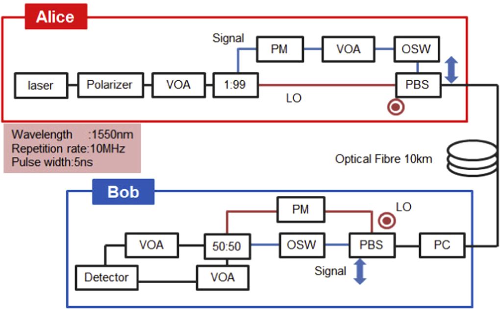
Figure 7 shows the schematic of our optical setup. The optical system includes Alice's and Bob's apparatus, and quantum channel. All of components in the optical system including a homodyne receiver are off-the-shelf fibre components and commercially available. We use a DFB laser of 1550 nm wavelength as a light source. Repetition frequency of the light pulse is 10 MHz and the pulse duration is 5 nsec. The optical configuration is a polarisation and time division multiplexed interferometer. In order to stabilise the relative phase between the signal and LO pulse, we packaged the interferometer part of Alice's and Bob's components with thermal insulation materials. Light pulse from the laser is split by a beam splitter of 1:99 ratio. Weaker light is used as the signal light and stronger light is as the LO. The signal light is randomly phase modulated into one of four states by a phase modulator (PM), then attenuated to an appropriate intensity by a variable optical attenuator (VOA). The signal and LO light enter an optical fibre with orthogonal linear polarisations and also with a time delay of about 50 nsec with each other. Since the polarisation is not maintained in the quantum channel, a polarisation controller (PL) is placed at the entrance of Bob's apparatus. Then, the LO and the signal are split by a polarising beam splitter (PBS). The LO light is randomly phase modulated by a PM: Bob randomly selects $x-$ or $p-$ measurement. Finally, the signal and LO are combined at a half beam splitter, and two outputs incident to two optical paths and reach balanced photo detectors and the quadrature amplitude of the signal light is measured by homodyne detection. Two VOAs in front of photo detectors are used to balance the light intensity of two outputs.

Zoom In Zoom Out Reset image size

Figure 8 shows the schematics of our CV-QKD system. Each station consists of three blocks; the optical system block, a control block, and a personal computer. From the optical block of Alice, quantum signals are sent to Bob, and they are received by the optical block of Bob. The components such as VOAs in optical blocks can be controlled by applying voltages from control blocks. The control blocks contain commercially available FPGA boards with daughter boards that perform Analogue-to-Digital conversion (ADC) and Digital-to-Analogue conversion (DAC) and are used to control the optical components in optical blocks. The FPGA boards operate with a master clock of 100 MHz which is generated by an oscillator. This clock is sent from Alice's block to Bob's block by 1310 nm light using Small Form-factor Pluggable (SFP) modules. The quantum signal and the clock light are transmitted over the same path by wavelength-division multiplexing (WDM). The control blocks are also equipped with ICs for generating random numbers. The random number generator ICs can generate physical random numbers at 1 Mbps. Pseudo-random numbers can be generated by FPGAs for 10 MHz operation. Personal computers (PC) and the FPGA boards are connected by USB cables. The output of the homodyne receiver is recorded by an ADC board connected to a PCI-express bus of the PC. PCs are also equipped with GPU cards to accelerate the software-based post-processing. We use non-binary LDPC code [34] for error correction (RR) and a fast privacy amplification algorithm using the Toeplitz matrix multiplication [35] (see appendix). Alice's station and Bob's station are enclosed in two 19-inch rack mounts as shown in figure 9.

Zoom In Zoom Out Reset image size

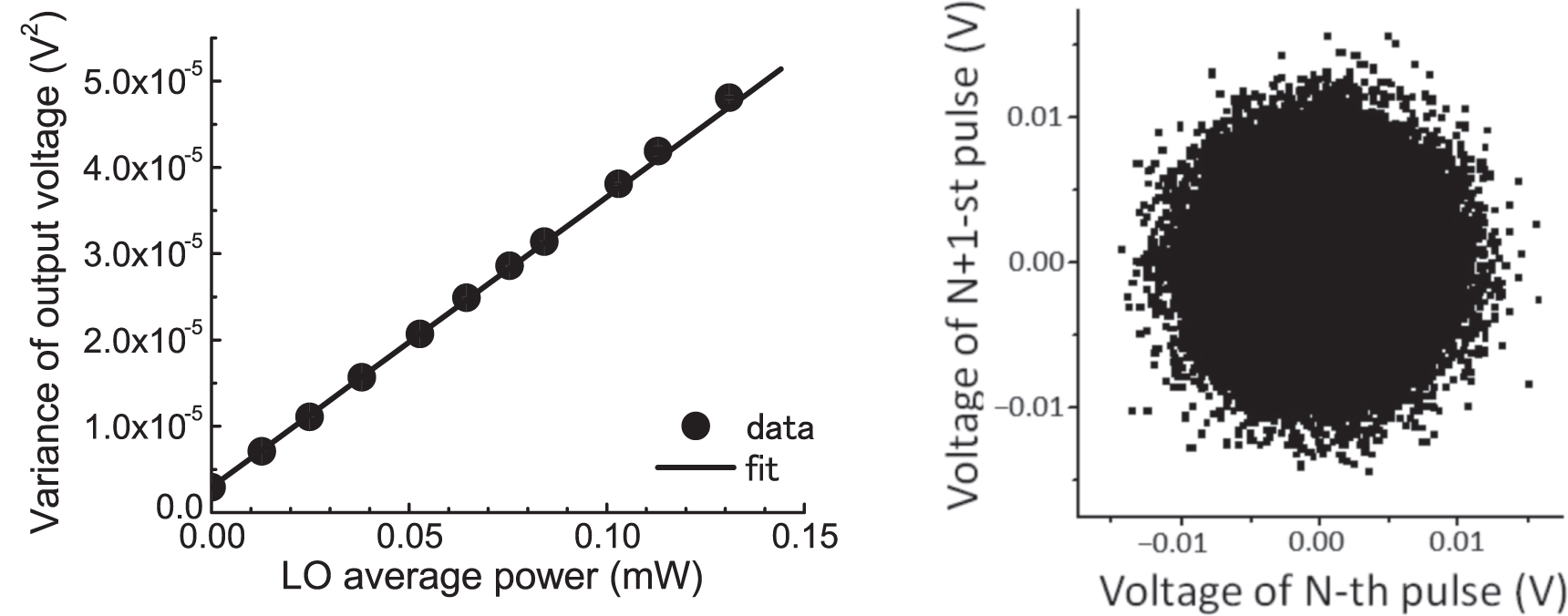
Zoom In Zoom Out Reset image size

Figure 10 shows the noise characteristics of the commercially available balanced receiver (General photonics, BPD-001-50) used for homodyne detection. In the figure on the left, the variance of the output voltage when the photo detectors are irradiated only by the LO is shown as a function of the average power of the LO light. As the average power of the LO increases, the variance of output voltage increases linearly. This linear dependence indicates that shot-noise-limited homodyne detection is possible using the commercial receiver. When the average power of the LO is 0.1 mW, the shot noise level is about 10 times larger than the dark noise of the receiver.

Zoom In Zoom Out Reset image size

In the time domain, correlation between measured values of the N-th pulse and the (N + 1)-st pulse was investigated in order to know whether adjacent pulses could be measured independently. In the right of figure 10 we observe an isotropic distribution and the correlation coefficient of the data is less than 0.01, indicating that each pulse light can be independently measured.

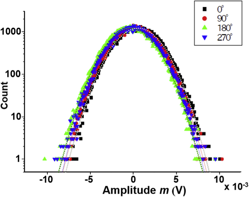
In figure 11, typical distributions of the voltage output of the homodyne receiver for four kinds of relative phase between the signal and LO are shown in a semi-log scale. We can see that these distributions are well represented by Gaussian distribution. The average values of the amplitude m for 90 and 270 degrees data are almost zero, and those for 0 and 180 degrees data are plus and minus values, respectively.

Zoom In Zoom Out Reset image size

In the key generation operation, Alice sends 10⁶ pulses at a time and a half of them is used for the parameter estimation: In the parameter estimation, the mean values and variances of the measurement results for four kinds of relative phases are calculated. From these values, excess noise and transmissivity of the quantum channel can be evaluated. In addition, the relative phase offset between the signal and the LO is obtained and this offset value is used to stabilise the phase offset. At present, this procedure can be repeated every 0.3 seconds; the repetition time is limited by the transfer time of random numbers from Alice's FPGA board to Alice's PC through a USB cable. By improving the transfer rate, three times faster operation will be possible.

6.1. Optical phase tracking

The optical system shown in figure 7 is basically a Mach-Zehnder interferometer. The relative phase between the signal and LO should be kept stable with higher accuracy than the wavelength of the light. Especially in the case of CV-QKD, the relative phase variation must be made very small in order to keep excess noise small.

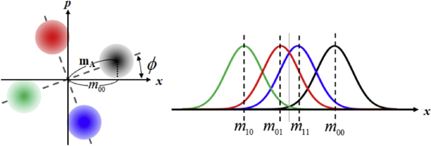
The relative phase offset between the signal and LO can be estimated relatively easily in four-state CV-QKD. In figure 12, the effect of phase offset is schematically shown. Let be the average value of the measured voltage for the relative phase ${\theta }_{{ij}}=i\times \pi +j\times \pi /2$ ($i,j=0$ or 1) ${m}_{{ij}}={m}_{A}\cos ({\theta }_{{ij}}+\phi )$, here ${m}_{A}$ is the amplitude of the signal and ϕ is the phase offset. Then, from the measured average values m_ij, the amplitude ${m}_{A}$ is calculated as ${m}_{A}=\sqrt{\sum {m}_{{ij}}^{2}/2}$ and the phase offset ϕ is calculated as the average of arccos $({m}_{{ij}}/{m}_{A})-{\theta }_{{ij}}$. This phase offset value is fed to the voltage of the phase modulator in Bob's optical box. Typical phase fluctuation after stabilisation is 0.05 radian. Excess noise can be kept less that 0.02 for most of the time. When the phase offset is suddenly increased, such data are discarded.

Zoom In Zoom Out Reset image size

6.2. Real-time key generation

In a real operation, it is necessary to take account the efficiency of the error correction in the secret fraction. When the error correction efficiency f is not unity, the mutual information between Alice and Bob is given as

$$\begin{eqnarray}&&{I}_{\mathrm{AB}}^{\prime }=1-{fh}(\epsilon ).\end{eqnarray} \tag{ 5’ }$$

Then the secret fraction is modified to $r^{\prime} =\int {dm}\,P(m| \alpha ){\rm{\Delta }}I^{\prime}$, where ${\rm{\Delta }}I^{\prime} ={I}_{\mathrm{AB}}^{\prime} -\chi$ and the integral is taken over the region where ${\rm{\Delta }}I^{\prime} \geqslant 0$. The compression factor of the classical post-processing, ${r}_{\mathrm{comp}}$, is defined as the ratio of the secret fraction to the post-selection rate p:

$$\begin{eqnarray}&&{r}_{\mathrm{comp}}=r^{\prime} /p.\end{eqnarray} \tag{ 38 }$$

Table 1 shows numerical examples of the post-selection rate and the compression factor. In this numerical calculation, the channel loss is 0.2 dB/km, the error correction efficiency is f = 1.3, and the signal photon number $| \alpha {| }^{2}$ is optimised.

Table 1.  Post-selection rate and compression factor. Error correction efficiency f is set to be 1.3.

Excess noise	Distance(km)	Photon number	p	${r}_{\mathrm{comp}}$
0.5%	1	4.3	0.960208	0.648948
	5	2.7	0.820866	0.349567
	10	2.2	0.64053	0.214132
1%	1	4.2	0.956934	0.624086
	5	2.7	0.817244	0.336959
	10	2.2	0.631302	0.203932
2%	1	4.1	0.952484	0.578773
	5	2.8	0.818266	0.310443
	10	2.3	0.624872	0.182115

Figure 13 shows an example of key generation results. This is the data when the CV-QKD system was installed in the NICT facility and connected to the Tokyo QKD network [36, 37]. The quantum channel is a 10 km optical fibre. Sift key rate is about 300 kbps and secure key rate is about 50 kbps.

Zoom In Zoom Out Reset image size

We performed RR using non-binary LDPC code [34]. The error correction efficiency parameter was set to be 1.3 although the code can operate stably even when the f parameter is 1.08 and error rate is 0.15. The speed of error correction is about 300 kbps per thread using a GPU (GTX 680). Privacy amplification was performed by Toeplitz matrix multiplication [35]. Its calculation complexity can be reduced to $O(n\mathrm{log}n)$ for an input length n by exploiting the FFT algorithm.

In an automated operation, the compression factor is calculated by using a linear approximation function for numerical calculation shown in table 1, that gives the compression factor as functions of transmissivity and excess noise. Here we assume that Eve cannot control Bob's receiver which has optical loss and excess noise. We also assume that Eve's knowledge about the sift key when Bob has an ideal receiver is smaller than her knowledge about the sift key when Bob uses a lossy and noisy receiver because in the RR Eve has to infer lossy and noisy signal in the latter situation. Under these assumptions, the Holevo quantity in the former situation, χ, should be larger than that in the latter situation, $\chi ^{\prime}$:

$$\begin{eqnarray}&&\chi \geqslant \chi ^{\prime} .\end{eqnarray} \tag{ 39 }$$

In addition, we assume that the mutual information between Alice and Bob in the latter situation, ${H}_{\mathrm{AB}}^{\prime }$, is larger than that in the former situation, ${H}_{\mathrm{AB}}$:

$$\begin{eqnarray}&&{H}_{\mathrm{AB}}^{\prime }\geqslant {H}_{\mathrm{AB}}.\end{eqnarray} \tag{ 40 }$$

This assumption on mutual information can be satisfied when the error rate in the latter case (actual experiment) is set be smaller than that in the former case (ideal calculation) by increasing the threshold of post-selection. When equations (39) and (40) are satisfied, the following equation holds;

$$\begin{eqnarray}&&{\rm{\Delta }}{I}^{\prime }={H}_{\mathrm{AB}}^{\prime }-\chi ^{\prime} \geqslant {H}_{\mathrm{AB}}-\chi ={\rm{\Delta }}I.\end{eqnarray} \tag{ 41 }$$

That means the compression factor shown in table 1 can be safely used for the actual experiment where Bob uses a lossy and noisy receiver. In the experiment, the post-selection rate was kept about 0.4 which is smaller than the numerical calculation shown in table 1.

We described the security and experimental implementation of the four-state CV-QKD protocol using post-selection. We evaluated the secret fraction of the protocol against a collective attack both for DR and RR. As the quantum channel becomes longer, RR yields better secret fraction than DR. When the distance is shorter than 30 km, the secret fraction is insensitive to the value of the excess noise and this makes experimental implementation easier.

We experimentally demonstrated automated secure key generation with a rate of 50 kbps when a quantum channel is a 10 km optical fibre. A commercially available balanced receiver is used to realise shot-noise-limited pulsed homodyne detection. We use a non-binary LDPC code for error correction and the Toeplitz matrix multiplication for privacy amplification. A GPU card is used to accelerate the software-based post-processing. Real-time stabilisation of relative phase between the signal and LO has been demonstrated. The present CV-QKD system is simple and can be built at low cost, and it is possible to achieve better performance in the future. We believe the present implementation will make a significant contribution toward practical popularisation of QKD.

This work was partially supported by the Commissioned Research of National Institute of Information and Communications Technology (NICT), Japan, and by ImPACT Program of Council for Science, Technology and Innovation (Cabinet Office, Government of Japan). TI is grateful to Hosho Katsura, Toshihiko Sasaki and Shu Tanaka for valuable discussions.

In this appendix, we explain details of software-based post-processing used in our system.

Appendix. Error correction by a non-binary LDPC code

Non-binary LDPC codes were invented by Gallager [38] and it was found by Davey and MacKay that it can show better performance than binary LDPC codes [39]. In the case of the LDPC codes, it is necessary to choose properly from a collection of codes that are optimised for multiple error rates. By utilising a rate-compatible non-binary LDPC code which supports a wide-range of rates, it is possible to simplify the error-correction system while achieving efficient information reconciliation [40].

Details of the error correction procedure used in the present CV-QKD system is as follows. After Bob and Alice obtained their sifted keys, i.e. after step (vi) explained in section 2, Bob has an n-bit binary string ${Y}^{n}={({Y}_{1},{Y}_{2},\; ,\; ,{Y}_{n})}^{T}$ and Alice has ${X}^{n}={({X}_{1},{X}_{2},\; ,\; ,{X}_{n})}^{T}$. They know an estimate of bit error rate of their sift keys. In the reverse reconciliation scenario, the goal of the error correction is for Alice to reproduce a string ${\hat{Y}}^{n}$ by conversation with Bob over a public channel. The content of the conversation depends on ${Y}^{n}$, and $c({Y}^{n})$ denotes the content of the conversation. The error correction should have the following properties:

• the probability of ${Y}^{n}\ne {\hat{Y}}^{n}$ is sufficiently close to zero; and
• the mutual information $I({Y}^{n};c({Y}^{n})))$ is as small as possible.

The second property is important because Alice and Bob must subtract $I({Y}^{n};c({Y}^{n})))$ bits from the corrected key during the privacy amplification procedure as $I({Y}^{n};c({Y}^{n})))$ is the amount of information leaked to Eve during the conversation over the public channel. We can use a good error correction method by saving the number of bits in $c({Y}^{n})$ while enabling Alice to decode ${Y}^{n}$ from ${X}^{n}$ and $c({Y}^{n})$.

Schematics of the reverse reconciliation by an asymmetric coding is shown in figure 14 [40]. The encoder only uses ${Y}^{n}$ for generating the codeword $f({Y}^{n})$. The decoder uses both $f({Y}^{n})$ and ${X}^{n}$. In the reverse reconciliation, Bob has ${Y}^{n}$ and Alice has ${X}^{n}$. Therefore, Bob generates the codewords $f({Y}^{n})$ from ${Y}^{n}$ and sends $f({Y}^{n})$ to Alice. Then Alice uses the decoder for recovering ${Y}^{n}$. The amount of information leaked to Eve is estimated as $I({Y}^{n};f({Y}^{n}))\leqslant H(f({Y}^{n})\,\leqslant$ the number of bits in $f({Y}^{n})$. If the length of $f({Y}^{n})$ is shorter, upper bound on the leaked information is smaller. LDPC codes can be used for the asymmetric coding [41]. At some fixed rate, the information bits are encoded as a syndrome of an irregular LDPC code. The information can be estimated by an efficient algorithm, belief propagation decoding, with a help from the syndrome and the correlated information. However, in an actual QKD system, the bit error rate of the sift keys may fluctuate with time. In this case, the encoder and decoder must be equipped with multiple LDPC codes: each irregular LDPC code of channel coding rate R_c is designed to have lower decoding error probability over channel with $H(Y| X)$ which is as close to the bound $1-{R}_{c}$ as possible. A rate-adaptive error correction scheme with a set of optimised irregular LDPC codes for multiple channel coding rates were proposed by Elkouss et al [42]. However, since the number of LDPC codes equipped is limited in an actual QKD system, Alice and Bob have to use one of the LDPC codes equipped that may have degraded performance for the actual sift-key data. This degradation leads to the so-called saw effect [42].

Zoom In Zoom Out Reset image size

A rate-compatible coding uses only a single mother LDPC code and can solve the issue of the saw effect. Two of the authors of this paper (KK and RM) and Sakaniwa proposed an error correction scheme in conjunction with rate-compatible non-binary LDPC codes [40]. The (2,d_c)-regular non-binary LDPC code on the Galois field GF(2^p) with ${2}^{p}\geqslant 64$ are empirically known as the best performing error-correction codes. In the present CV-QKD implementation, we use a (2, 3)-regular non-binary LDPC code on GF(256). The main shortcoming of non-binary LDPC codes is decoding complexity. We use an programme that uses GPUs for faster processing. The programme can be downloaded from one of the authors (KK) web site [34].

Appendix. Privacy amplification using Toeplitz matrix multiplication

Privacy amplification is a procedure to extract random numbers unknown to third parties by applying a random hash function to a random source which may be partially leaked to third parties. This procedure is realised with a help of another auxiliary random source which is public and called a random seed. The most typical random hash function for this purpose is the universal₂ hash function, and the most widely used of it is the one using the (modified) Toeplitz matrix [35]. The hash function using the Toeplitz matrix allows an efficient implementation with complexity of $O(n\mathrm{log}n)$ for input length n and with a short seed length.

The Toeplitz matrix is a matrix whose diagonal elements are all same. It is parametrised by $r=({r}_{1},{r}_{2},\; ,\; ,\; ,{r}_{n-1})\in \{0,1\}{}^{n-1}$ as

$$\begin{eqnarray}T(r)=\left(\begin{array}{cccc}{r}_{m} & {r}_{m+1} & \cdots & {r}_{n-1}\\ {r}_{m-1} & {r}_{m} & \cdots & {r}_{n-2}\\ \vdots & \vdots & \ddots & \vdots \\ {r}_{1} & {r}_{2} & \cdots & {r}_{n-m-1}\end{array}\right).\end{eqnarray} \tag{ 42 }$$

For example, a multiplication of a 3 × 4 Toeplitz matrix and a four-element vector $z={({z}_{1},{z}_{2},{z}_{3},{z}_{4})}^{T}$ outputting a three-element vector $y={({y}_{1},{y}_{2},{y}_{3})}^{T}$ is written as

$$\begin{eqnarray}&&\left(\begin{array}{c}{y}_{1}\\ {y}_{2}\\ {y}_{3}\end{array}\right)=\left(\begin{array}{cccc}{r}_{3} & {r}_{4} & {r}_{5} & {r}_{6}\\ {r}_{2} & {r}_{3} & {r}_{4} & {r}_{5}\\ {r}_{1} & {r}_{2} & {r}_{3} & {r}_{4}\end{array}\right)\left(\begin{array}{c}{z}_{1}\\ {z}_{2}\\ {z}_{3}\\ {z}_{4}\end{array}\right).\end{eqnarray} \tag{ 43 }$$

This can be embedded in a multiplication of a square matrix and a vector by concatenating extra elements to vectors $y,z$ as

$$\begin{eqnarray}&&\left(\begin{array}{c}{y}_{1}\\ {y}_{2}\\ {y}_{3}\\ \ast \\ \ast \\ \ast \end{array}\right)=\left(\begin{array}{cccccc}{r}_{3} & {r}_{4} & {r}_{5} & {r}_{6} & {r}_{1} & {r}_{2}\\ {r}_{2} & {r}_{3} & {r}_{4} & {r}_{5} & {r}_{6} & {r}_{1}\\ {r}_{1} & {r}_{2} & {r}_{3} & {r}_{4} & {r}_{5} & {r}_{6}\\ {r}_{6} & {r}_{1} & {r}_{2} & {r}_{3} & {r}_{4} & {r}_{5}\\ {r}_{5} & {r}_{6} & {r}_{1} & {r}_{2} & {r}_{3} & {r}_{4}\\ {r}_{4} & {r}_{5} & {r}_{6} & {r}_{1} & {r}_{2} & {r}_{3}\end{array}\right)\left(\begin{array}{c}{z}_{1}\\ {z}_{2}\\ {z}_{3}\\ {z}_{4}\\ 0\\ 0\end{array}\right).\end{eqnarray} \tag{ 44 }$$

As explained in appendix C of [35], a multiplication of a square Toeplitz matrix and a vector can be performed by three calculations, i. e., two discrete Fourier transforms (DFT), a convolution and an inverse Fourier transform. Since the complexity of a DFT is $O(n\mathrm{log}n)$ using the FFT algorithm and the complexity of convolution is O(n), the total complexity of the multiplication is $O(n\mathrm{log}n)$.