Non-equilibrium Green function method: theory and application in simulation of nanometer electronic devices

For five decades of development, the 'non-equilibrium Green function' (NEGF) formalism has become a useful and powerful calculation/computation method to the study of dynamical processes in non-equilibrium many-body systems. Historically, the NEGF theory stems from efforts in applying ideas established in the quantum field theory to treat problems in statistical physics. Accordingly, the expectation values of observables and the correlation functions between observables can be systematically determined if knowing Green functions which are appropriately defined. For instance, the correlation function between the two observables $a$ and $b$ measured in a system wherein a ground state $\left| {{\Phi }_{0}} \right\rangle ,$ or a thermal-equilibrium state are established, can be calculated through the two-time Green function defined by [1–5]

$$\begin{eqnarray}\begin{array}{lllllllllllllll} {{G}_{ab}}(t,t\prime ) & = & -\frac{i}{\hbar }\langle \hat{T}\hat{a}(t)\hat{b}(t\prime )\rangle \\ {} & = & \left\{ \begin{array}{lllllllllllllll} -\frac{i}{\hbar }\left\langle {{\Phi }_{0}} \right|\hat{T}\hat{a}(t)\hat{b}(t\prime )\left| {{\Phi }_{0}} \right\rangle & \beta \to \infty \\ -\frac{i}{\hbar }\frac{\{{{{\mbox{e}}}^{-\beta H}}\hat{T}\hat{a}(t)\hat{b}(t\prime )\}}{\{{{{\mbox{e}}}^{-\beta H}}\}} & \beta \ne 0 \\ \end{array} \right. \\ \end{array}\end{eqnarray} \tag{ 1 }$$

where $\hat{a}$ and $\hat{b}$ are the operators defining the two quantities $a$ and $b,$ $\hat{T}$ denotes the arrangement of the operators $\hat{a}$ and $\hat{b}$ according to the order of their time variables $t$ and $t\prime$ on the real-time axis, $\{\ldots \}$ the trace operation as convention, $\hbar$ the reduced Planck constant and $\beta =1/{{k}_{B}}T$ the inversion of the thermal energy.

For the progress of the field, one should mention to the key contributions of Martin and Schwinger in the formulation of the general formalism of the N-particle Green function [6]. However, in the practical point of view, in order to calculate such N-particle Green functions one needs to introduce appropriate approximations, which usually lead to the appearance of many novel correlation functions. In 1961, Kadanoff and Baym discussed some fundamental aspects in the implementation of the Martin-Schwinger theory in the view point of macroscopic conservation laws, the continuity equation for instance [7]. The development of the quantum field theory for thermal equilibrium many-body systems led to the formulation of the temperature Matsubara Green function theory. This theory is based on the concept of imaginary time, which was introduced based on the analogy between the time evolution operator and the equilibrium statistical one [2–4]. However, different from the equilibrium situation, non-equilibrium systems do not have neither a ground state nor a unique statistical operator. Treatment of such systems therefore requires the introduction of novel Green functions to quantify typical statistical properties such as the distribution of particles on the spectrum of microscopic states. In 1965, Keldysh introduced a way to unify a class of four basic two time-variables Green functions using the concept of time-contour [8], defined on which is the time-contour Green function or the Keldysh Green function. Inversely, by making the continuum limit, which is expressed through the so-called Langreth theorem [9], the time-contour Green function leads to a set of four real-time two-point Green functions, which simultaneously describe the two fundamental aspects of many-body systems: the spectrum of quantum states of particles and the state populations or the average number of particles occupying each state. These real-time two-point Green functions are thus able to describe generally many-body systems without needing the distinction of their statistical state, i.e., equilibrium or non-equilibrium. Since 2000, a series of conferences had been held to report progresses and to sketch perspectives of the NEGF theory. Collections of papers published in a series of proceedings named 'Progress in Non-equilibrium Green functions' report interesting key results and breakthroughs in applying this method to various fields such as plasma physics, solid state theory, semiconductor optics and transport, nanostructures, nuclear matter and even high energy physics [10].

In the last decade, the NEGF method has been developed to investigate and predict transport properties of nanoscale materials as well as the operation and the performance of nanoscale devices. The NEGF method has been implemented into many computer packages with different sophisticated levels, for instance, combined with density-functional calculations [11–13], or based on effective physical models [14–17]. However, many technical and physical issues still need to be solved to improve the effectiveness and the performance of such computational tools in various applications. Our computer package named OPEDEVS, standing for 'Opto and Electronic Device Simulation' [18], has been recently developed on the basis of the NEGF method to the study of the electronic and transport properties of nanoscale materials and devices with different geometrical structures. The purpose of this paper is therefore to present a short review of fundamental aspects in the implementation of the NEGF method into the OPEDEVS package. Nevertheless, all basic concepts and key equations of the theory are presented in detail, in a more suitable form for the computational purposes rather than for a full description of the theory.

The layout of the paper is presented as follows. In section 2, we review progresses in the last decades of the NEGF method in nano-electronics. In section 3 we present the definition of the four real-time Green functions, viz the retarded, advanced, lesser and greater ones, and their equations of motion and basic relations among them. In particular, we discuss the issue of how to calculate important physical quantities from the Green functions in the quantification of the transport properties of nano-electronic systems. In section 4, two efficient recursive algorithms are presented, which are implemented in the OPEDEVS package, to solve the Green functions defined in finite-size opened systems and in the surface layer of semi infinite-size homogeneous systems. Section 5 is dedicated to the illustration of the application of OPEDEVS to study a typical semiconductor device structure, the resonant tunneling diode (RTD). Section 6 concludes the paper.

Since the invention in 1962, the technology based on the complementary metal-oxide-semiconductor (CMOS) circuit, named the CMOS technology, has been rapidly and strongly developed in the trend of minimizing the size of the building blocks such as the p- and n-type metal-oxide-semiconductor field-effect transistors (MOSFETs). This trend, however, for the last decades, revealed severe obstacles generally known as the short-channel effects, when the device gate length approaches the nanometer scales. Though the 30 nm technology (implying that the typical length of the gate electrode of the MOSFET structure is about 30 nm) had been started since 2007, the International Technology Roadmap for Semiconductors [19] predicts that this trend will be soon stopped, because of the non-preservation of the transfer characteristics as those of conventional device structures. Fundamentally, such problems originated from the emergence of quantum effects that limit the device scaling trend.

Therefore, it has been crucial to study quantum behaviors and transport mechanisms of charge carriers which govern the characteristics of nano-scale devices. On the one hand, that research helps clarifying the lower limit of the scaling process. On another hand, it may shed light on the finding of alternative fabrication methods, and even on the invention of novel device generations. In such context, it is necessary to develop efficient theoretical approaches and powerful computational tools to study rigorously the role of quantum effects involving in the transport of charge carriers in nano-scale device structures, and hence their dominant influence on the device performance.

Figure 1(a) illustrates a typical device structure of two terminals. The central region is called the active one that governs the behaviors of the whole device, while the two end regions, called the leads, play the role of the source and the sink of charge carriers. The active region is thus considered as an opened system which communicates with its environment via the leads. At the scales of conventional device structures, with the gate length in the order of $1\;\mu {\mbox{m}},$ various classical and semi-classical approaches, for instance, the drift-diffusion model and/or the ones based on the semi-classical Boltzmann equation, have been developed [20]. Such approaches, however, become invalid in capturing the quantum effects, such as the quantum interference, confinement and tunneling, which become emerging when the size of the devices is comparable to, or even smaller than, the phase breaking length ${{L}_{\phi }}$ of charge carriers. When the wave function of carriers can extend largely over the central region to the leads, carriers can move coherently through the whole device. The transport, in this sense, is said to be in the coherent regime, or in the ballistic transport regime. The current of charge carriers flowing through the structure therefore can be determined by a rather simple and intuitive formula introduced by Landauer in 1947, which was then validated and generalized for multi-probe systems by Buttiker using the framework of the scattering theory [21–24],

$$\begin{eqnarray}&&I=\frac{{{e}_{0}}}{\hbar }\int \frac{{\mbox{d}}E}{2\pi }\mathcal{T}(E)\left[ {{n}_{L}}(E)-{{n}_{R}}(E) \right],\end{eqnarray} \tag{ 2 }$$

where ${{e}_{0}}$ is the absolute value of the electron charge, and $\mathcal{T}(E)$ is called the transmission coefficient, which is actually the summation of transmission probabilities (the transmittances) of charge carriers over all possible single-particle modes. The transmission coefficient is therefore a physical quantity quantifying the 'transparency' of the opened system, which is viewed as the agent scattering the carrier plane waves incident from the terminal regions. In the above equation, the role of the carrier source (the left-$L$) and sink (the right-$R$) regions is explicitly reflected through the presence of the two functions ${{n}_{L}}(E)$ and ${{n}_{R}}(E)$ which define the average occupation number of carriers on states with energy $E.$ Since these regions are usually much larger than the device active one, they are usually assumed to be in a thermal equilibrium state, and thus characterized by a temperature ${{T}_{\nu }}$ and a chemical potential ${{\mu }_{\nu }}$ $\left( \nu =L,R \right).$ In practice, the functions ${{n}_{L/R}}(E)$ are usually approximated by the Fermi–Dirac function with some special notices involving in the specific value of the temperature and the chemical potential [25]. The calculation of the current of charge carriers by equation (2) therefore revolves around the determination of the transmission coefficient. Different methods may be used to this aim, including the use of the scattering method with the help of the transfer matrix technique [26], or the use of the real-space Green function method associated with the Fisher–Lee relation [27].

Zoom In Zoom Out Reset image size

Though equation (2) is useful, it is based on the single-particle picture. In practice, even when the ballistic and coherent transport regime dominate in the nanoscale structures, the problem of carriers scattering off impurities, lattice vibrations, and the surfaces/interfaces in/of material layers is in general inevitable. These scattering processes may even govern typical behaviors of devices, for instance, the effect of phonon-assistance transport and the super-Poissonian noise in double-barrier resonant tunneling structures [28]. Such effects apparently cannot be microscopically accounted for in the framework of the Landauer–Buttiker formalism (the scattering theory). A general theory that enables naturally connecting the two transport regimes, i.e., the ballistic and the diffusion ones, is therefore needed.

To the simulation of electronic device structures, the transport equations of charge carriers, in principle, must be presented and solved in the real time-space. In 1990, Caroli pointed out that some physical quantities quantifying the transport characteristics of an opened system can be expressed in terms of the Green functions which are defined only in the active region [29]. In 1992, Meir and Wingreen based on the NEGF formalism to formulate an expression for the charge current flowing through a finite scattering region and recovered the well-known Landauer formula in the limit of no-scattering, i.e., in the coherent transport regime [30]. In the next sections, we will review these key results since they play the basic role in the development of the NEGF formalism for the device simulation. In 1995, Datta introduced a book wherein many practical aspects of implementing the NEGF method are discussed in a rather pedagogical way using the matrix representation of the Green functions of the two terminal structures [31].

Practically, the most difficult part in the use of the NEGF method for investigating transport properties of a system lies in the treatment of many-particle interaction effects. Diagram techniques developed for the many-body Green functions in general can be used in the NEGF formalism. It, however, is a formidable task [4]. For the cases in which interaction processes play the role of making the transition of particle from one state to another, but do not cause significant changes in the dispersion relation, the NEGF formalism can be used in the quantum-version form of the Boltzmann equation for the so-called Wigner function [32]. Mathematically, the Wigner function plays the role similar to the Boltzmann distribution function in the determination of the kinetic properties of a quantum system, but it is not positively defined. In addition, since the transition processes can be treated using the framework of the Fermi golden rule, many useful methods and techniques already developed in the classical statistics, such as the Monte–Carlo method, can be used to solve the quantum Boltzmann equation [33, 34].

Regarding the solution of the NEGFs, it is worth noting their recursive structure in terms of the so-called Dyson equation. The fact is that the realization of a mathematical structure in a system of equations will strongly facilitates computational processes. This point will be detailed in section 4, but informatively, it should mention some important contributions in the field of numerical calculations. In 1997, Lake et al. successfully used the recursive method to calculate all diagonal elements of the retarded Green function matrix defined in the device active region [14]. This technique enables combining different parts of a whole device using the concept of coupling self-energy. In 2002, Svizhenko et al. started from the matrix structure of the transport equations to introduce a rather general algorithm to compute not only important elements of the retarded/advanced Green functions but also of the other correlation functions, i.e., the lesser and greater Green functions (see next section) [15]. This algorithm is very useful and now commonly used to find, in a systematic way, all of the Green functions defined in the device active region given the self-energies characterizing the terminal (source/sink) regions. For some simple transport models, such coupling self-energies can be analytically found [26, 31]. However, when dealing with complicated models, such as multi-bands and/or atomic tight-binding description, it is not easy to handle the analytical calculations. The algorithm proposed by Sancho and Rubio in 1984 to treat semi-infinite systems was usually revisited. It is now known as a rather general, stable and efficient method to calculate the coupling self-energies [35]. All these techniques are the key ingredients for the implementation of the NEGF method to the problem of quantum device simulation. In the next sections we will review these points, which have been successfully implemented in the OPEDEVS package.

3.1. Definitions

Given an electron system which is described by a Hamiltonian $\hat{H}$ represented in terms of the field operators ${{\hat{c}}_{\alpha }},\hat{c}_{\beta }^{\dagger },$ where $\alpha$ and $\beta$ denote, for short, the sets of quantum indices labeling quantum states of the system. The time-contour Keldysh Green function is defined by (see appendix A):

$$\begin{eqnarray}&&G_{\alpha ,\beta }^{\mathcal{C}}({{\tau }_{1}};{{\tau }_{2}})=-\frac{i}{\hbar }\left\langle {{\hat{T}}_{\mathcal{C}}}{{\hat{c}}_{\alpha }}({{\tau }_{1}})\hat{c}_{\beta }^{\dagger }({{\tau }_{2}}) \right\rangle ,\end{eqnarray} \tag{ 3 }$$

wherein $\mathcal{C}$ denotes the time-contour such that ${{\tau }_{1}},{{\tau }_{2}}\in \mathcal{C}$ (see figures 2(a) and (b)), ${{\hat{T}}_{\mathcal{C}}}$ is the time-ordering operator on the time-contour, and the angle bracket denotes the ensemble average as specified in equation (1). The time-contour $\mathcal{C}$ can be seen as composed of three branches ${{\mathcal{C}}_{1}}=(-\infty +i\eta ,+\infty +i\eta ),$ ${{\mathcal{C}}_{2}}=(+\infty -i\eta ,{{t}_{0}}-i\eta )$ and ${{\mathcal{C}}_{3}}=({{t}_{0}}-i\eta ,{{t}_{0}}-i\beta )$ where $\eta >0$ and $\beta =1/{{k}_{B}}T.$ The complex time variables ${{\tau }_{1}},{{\tau }_{2}}$ in equation (3) therefore can be specified as $\tau =t+i\eta$ if $\tau \in {{C}_{1}},$ $\tau =t-i\eta$ if $\tau \in {{C}_{2}},$ and $\tau ={{t}_{0}}-it$ if $\tau \in {{C}_{3}}.$

Zoom In Zoom Out Reset image size

The definition of the NEGF given by equation (3) actually is the general one for the four real-time Green functions: the lesser $\left( < \right),$ greater $\left( > \right),$ causal (time-ordered) $\left( c \right)$ and anti-causal (anti time-ordered) $\left( {\bar{c}} \right)$ Green functions when taking the limit $\eta \to 0$ [2–4]:

$$\begin{eqnarray}&&\begin{array}{lllllllllllllll} G_{\alpha ,\beta }^{\mathcal{C}}(\tau ,\tau \prime )= \\ \quad \left\{ \begin{array}{lllllllllllllll} G_{\alpha ,\beta }^{c}(t,t\prime )=-\frac{i}{\hbar }\left\langle \hat{T}{{\hat{c}}_{\alpha }}(t)\hat{c}_{\beta }^{\dagger }(t\prime ) \right\rangle & \tau \in {{\mathcal{C}}_{1}} & \And & \tau \prime \in {{\mathcal{C}}_{1}} \\ G_{\alpha ,\beta }^{<}(t,t\prime )=+\frac{i}{\hbar }\left\langle \hat{c}_{\beta }^{\dagger }(t\prime ){{\hat{c}}_{\alpha }}(t) \right\rangle & \tau \in {{\mathcal{C}}_{1}} & \And & \tau \prime \in {{\mathcal{C}}_{2}} \\ G_{\alpha ,\beta }^{>}(t,t\prime )=-\frac{i}{\hbar }\left\langle {{\hat{c}}_{\alpha }}(t)\hat{c}_{\beta }^{\dagger }(t\prime ) \right\rangle & \tau \in {{\mathcal{C}}_{2}} & \And & \tau \prime \in {{\mathcal{C}}_{1}} \\ G_{\alpha ,\beta }^{{\bar{c}}}(t,t\prime )=-\frac{i}{\hbar }\left\langle \mathop{{\bar{T}}}\limits^{\hat}{{\hat{c}}_{\alpha }}(t)\hat{c}_{\beta }^{\dagger }(t\prime ) \right\rangle & \tau \in {{\mathcal{C}}_{2}} & \And & \tau \prime \in {{\mathcal{C}}_{2}} \\ \end{array} \right. \\ \end{array}\end{eqnarray} \tag{ 4 }$$

By the definition, the causal and anti-causal Green functions $G_{\alpha ,\beta }^{c}(t,t\prime )$ and $G_{\alpha ,\beta }^{{\bar{c}}}(t,t\prime )$ are related to the functions $G_{\alpha ,\beta }^{<}(t,t\prime )$ and $G_{\alpha ,\beta }^{>}(t,t\prime )$ by the expressions:

$$\begin{eqnarray}&&G_{\alpha ,\beta }^{c}(t,t\prime )=\theta (t-t\prime )G_{\alpha ,\beta }^{>}(t,t\prime )+\theta (t\prime -t)G_{\alpha ,\beta }^{<}(t,t\prime )\end{eqnarray} \tag{ 5 }$$

$$\begin{eqnarray}&&G_{\alpha ,\beta }^{{\bar{c}}}(t,t\prime )=\theta (t\prime -t)G_{\alpha ,\beta }^{>}(t,t\prime )+\theta (t-t\prime )G_{\alpha ,\beta }^{<}(t,t\prime ),\end{eqnarray} \tag{ 6 }$$

where $\theta$ is the step function as convention. On the branch ${{\mathcal{C}}_{3}}$ we obtain the Matsubara Green function [2, 3].

Practically, one usually does not work with the causal and anti-causal Green functions (due to their analytical properties) [2, 3]. The two other real-time Green functions, the retarded $G_{\alpha ,\beta }^{r}$ and the advanced $G_{\alpha ,\beta }^{a}$ ones, are used instead:

$$\begin{eqnarray}\begin{array}{lllllllllllllll} G_{\alpha ,\beta }^{r}\left( t,t\prime \right) & = & -\frac{i}{\hbar }\left\langle \left\{ {{\hat{c}}_{\alpha }}(t),\hat{c}_{\beta }^{\dagger }(t\prime ) \right\} \right\rangle \theta \left( t-t\prime \right) \\ {} & = & \theta \left( t-t\prime \right)\left[ G_{\alpha ,\beta }^{>}(t,t\prime )-G_{\alpha ,\beta }^{<}(t,t\prime ) \right] \\ \end{array}\end{eqnarray} \tag{ 7 }$$

$$\begin{eqnarray}\begin{array}{lllllllllllllll} G_{\alpha ,\beta }^{a}(t,t\prime ) & = & +\frac{i}{\hbar }\left\langle \left\{ {{\hat{c}}_{\alpha }}(t),\hat{c}_{\beta }^{\dagger }(t\prime ) \right\} \right\rangle \theta (t\prime -t) \\ {} & = & \theta (t\prime -t)\left[ G_{\alpha ,\beta }^{<}(t,t\prime )-G_{\alpha ,\beta }^{>}(t,t\prime ) \right] \\ \end{array}\end{eqnarray} \tag{ 8 }$$

where the curly bracket denotes the anti-commutator.

From equations (5)–(8) we clearly realize the general relationships among the four real-time functions:

$$\begin{eqnarray}&&G_{\alpha ,\beta }^{c}+G_{\alpha ,\beta }^{{\bar{c}}}=G_{\alpha ,\beta }^{>}+G_{\alpha ,\beta }^{<}\end{eqnarray} \tag{ 9 }$$

$$\begin{eqnarray}&&G_{\alpha ,\beta }^{r}-G_{\alpha ,\beta }^{a}=G_{\alpha ,\beta }^{>}-G_{\alpha ,\beta }^{<}\end{eqnarray} \tag{ 10 }$$

$$\begin{eqnarray}&&G_{\alpha ,\beta }^{c}=G_{\alpha ,\beta }^{<}+G_{\alpha ,\beta }^{r}=G_{\alpha ,\beta }^{>}+G_{\alpha ,\beta }^{a}\end{eqnarray} \tag{ 11 }$$

$$\begin{eqnarray}&&G_{\alpha ,\beta }^{{\bar{c}}}=G_{\alpha ,\beta }^{<}-G_{\alpha ,\beta }^{a}=G_{\alpha ,\beta }^{>}-G_{\alpha ,\beta }^{r}\end{eqnarray} \tag{ 12 }$$

In most cases, we are usually interested in the steady state of a system. The two-time correlation/Green functions become dependent on only the difference between the two time variables $\bar{t}={{t}_{1}}-{{t}_{2}}.$ Therefore, it is more convenient to work with their Fourier transforms $\left\{ G_{\alpha ,\beta }^{\nu }(E) \right\},$ for instance,

$$\begin{eqnarray}&&G_{\alpha ,\beta }^{\nu }(E)=\int {\mbox{d}}({{t}_{1}}-{{t}_{2}}){{{\mbox{e}}}^{i\frac{E}{\hbar }\left( {{t}_{1}}-{{t}_{2}} \right)}}G_{\alpha ,\beta }^{\nu }({{t}_{1}}-{{t}_{2}}).\end{eqnarray} \tag{ 13 }$$

Inversely, we have

$$\begin{eqnarray}&&G_{\alpha ,\beta }^{\nu }({{t}_{1}},{{t}_{2}})=\int \frac{{\mbox{d}}E}{2\pi }{{{\mbox{e}}}^{-i\frac{E}{\hbar }({{t}_{1}}-{{t}_{2}})}}G_{\alpha ,\beta }^{\nu }(E)\end{eqnarray} \tag{ 14 }$$

In the above equations and so later, the superscript $\nu$ is used to denote the ones $\{\lessgtr ,r,a\}$ (except some cases which will be noted), and $E$ is the energy variable. Practically, it is useful to remark the dimension of the defined Green functions in equations (4) and (13). Since the field operators are usually chosen to be dimensionless, the real-time Green functions $G_{\alpha ,\beta }^{\nu }({{t}_{1}},{{t}_{2}})$ and their Fourier transforms $G_{\alpha ,\beta }^{\nu }(E),$ in 'the International System of units', therefore have the dimension of (J s)⁻¹ and J⁻¹, respectively.

For electron systems, it is worth to mention to the spectral density matrix ${{A}_{\alpha ,\beta }}(E),$ which is defined as follows

$$\begin{eqnarray}&&{{A}_{\alpha ,\beta }}(E)=i\left[ G_{\alpha ,\beta }^{r}(E)-G_{\alpha ,\beta }^{a}(E) \right]\end{eqnarray} \tag{ 15 }$$

$$\begin{eqnarray}&&=i\left[ G_{\alpha ,\beta }^{>}(E)-G_{\alpha ,\beta }^{<}(E) \right]\end{eqnarray} \tag{ 16 }$$

As generally presented in [2, 3] the diagonal elements, i.e., when $\alpha =\beta ,$ of this quantity are positively definite and provide information of the energy spectrum of elementary excitations in the systems. The spectral density matrix therefore has the dimension of the energy inversion.

3.2. Equations of motion

In appendix B we present the Dyson equations for the time-contour Green function ${{{\boldsymbol{G}} }^{\mathcal{C}}}(\tau ,\tau \prime )$ (In the following the bold characters are used to denote the matrix and vector notation, i.e., to omit quantum indices). Mathematically, it is an integral equation obtained from the perturbation expansion of equation (A.12). In this section, we will apply the Langreth theorem (proved in appendix B) to the Dyson equations (B.5) and (B.6), to specify the equations of motion, in the general form, for the four real-time Green functions, i.e., the retarded, advanced, lesser and greater.

Indeed, making use of the rules given in table B1, the continuum limit of equation (B.5) becomes [32]:

$$\begin{eqnarray}&&\begin{array}{lllllllllllllll} {{\mathop{\mathcal{G}}\limits^{\hat}}^{-1}}(t){{{\boldsymbol{G}} }^{r/a}}(t,t\prime )={\boldsymbol{ \delta }} (t-t\prime ) \\ \quad \quad \quad \quad \quad \quad +\int {\mbox{d}}{{t}_{2}}{{{\boldsymbol{ \Sigma }} }^{r/a}}(t,{{t}_{2}}){{{\boldsymbol{G}} }^{r/a}}({{t}_{2}},t\prime ), \\ \end{array}\end{eqnarray} \tag{ 17 }$$

$$\begin{eqnarray}&&\begin{array}{lllllllllllllll} {{\mathop{\mathcal{G}}\limits^{\hat}}^{-1}}(t){{{\boldsymbol{G}} }^{\lessgtr }}(t,t\prime ) \\ =\int {\mbox{d}}{{t}_{2}}\left[ {{{\boldsymbol{ \Sigma }} }^{r}}(t,{{t}_{2}}){{{\boldsymbol{G}} }^{\lessgtr }}({{t}_{2}},t\prime )+{{{\boldsymbol{ \Sigma }} }^{\lessgtr }}(t,{{t}_{2}}){{{\boldsymbol{G}} }^{a}}({{t}_{2}},t\prime ) \right] \\ \end{array}\end{eqnarray} \tag{ 18 }$$

Similarly, the continuum limit of equation (B.6) yields

$$\begin{eqnarray}&&\begin{array}{lllllllllllllll} {{{\boldsymbol{G}} }^{r/a}}(t,t\prime )\mathcal{G}{{\prime }^{-1}}(t\prime ) \\ \quad ={\boldsymbol{ \delta }} (t-t\prime )+\int {\mbox{d}}{{t}_{1}}{{{\boldsymbol{G}} }^{r/a}}(t,{{t}_{1}}){{{\boldsymbol{ \Sigma }} }^{r/a}}({{t}_{1}},t\prime ), \\ \end{array}\end{eqnarray} \tag{ 19 }$$

$$\begin{eqnarray}&&\begin{array}{lllllllllllllll} {{{\boldsymbol{G}} }^{\lessgtr }}(t,t\prime )\mathcal{G}{{\prime }^{-1}}(t\prime ) \\ =\int {\mbox{d}}{{t}_{1}}\left[ {{{\boldsymbol{G}} }^{r}}(t,{{t}_{1}}){{{\boldsymbol{ \Sigma }} }^{\lessgtr }}({{t}_{1}},t\prime )+{{{\boldsymbol{G}} }^{\lessgtr }}(t,{{t}_{1}}){{{\boldsymbol{ \Sigma }} }^{a}}({{t}_{1}},t\prime ) \right] \\ \end{array}\end{eqnarray} \tag{ 20 }$$

Because of the time-convolution integrals in the above equations, it is useful to write down the equations for the Fourier transforms of the Green functions. Straightforwardly, it results in

$$\begin{eqnarray}&&{{\mathcal{G}}^{-1}}(E){{{\mathbf{G}}}^{r/a}}(E)={\mathbf{I}}+{{\Sigma }^{r/a}}(E){{{\mathbf{G}}}^{r/a}}(E),\end{eqnarray} \tag{ 21 }$$

$$\begin{eqnarray}&&{{\mathcal{G}}^{-1}}(E){{{\mathbf{G}}}^{\lessgtr }}(E)={{\Sigma }^{r}}(E){{{\mathbf{G}}}^{\lessgtr }}(E)+{{\Sigma }^{\lessgtr }}(E){{{\mathbf{G}}}^{a}}(E),\end{eqnarray} \tag{ 22 }$$

and

$$\begin{eqnarray}&&{{{\mathbf{G}}}^{r/a}}(E)\mathcal{G}{{\prime }^{-1}}(E)={\mathbf{I}}+{{{\mathbf{G}}}^{r/a}}(E){{\Sigma }^{r/a}}(E),\end{eqnarray} \tag{ 23 }$$

$$\begin{eqnarray}&&{{{\mathbf{G}}}^{\lessgtr }}(E)\mathcal{G}{{\prime }^{-1}}(E)={{{\mathbf{G}}}^{r}}(E){{\Sigma }^{\lessgtr }}(E)+{{{\mathbf{G}}}^{\lessgtr }}(E){{\Sigma }^{a}}(E).\end{eqnarray} \tag{ 24 }$$

where ${{\mathcal{G}}^{-1}}(E)=\mathcal{G}{{\prime }^{-1}}(E)=(E+i\eta ){\mathbf{I}}-{{{\mathbf{H}}}_{0}}.$ Clearly, the obtained equations for the retarded/advanced, lesser and greater Green functions are not independent. In fact, they form a set of dependent integro-differential equations in the real-time representation, or a set of matrix equations in the energy representation. In section 4 we will present some useful algorithms to solve numerically these equations. To end this section, we would like to emphasize that all the above equations for the four real-time Green functions are exact and general in the meaning of the perturbation expansion, i.e., when one can define the self-energies. Given an expression for the full Hamiltonian $\hat{H}={{\hat{H}}_{0}}+{{\hat{H}}_{1}},$ the headache problem always is how to specify the self-energies. Technically, the self-energies can be constructed using the Feynman diagram technique [2, 3], or the method of equation of motion. These two are the most general, common and powerful techniques. For the latter, readers could consult [36] as an example.

3.3. Some basic properties and relations

In this section some general analytical properties of the Green functions are summarized. From the definition of the real-time Green functions, it is straightforward to check that

$$\begin{eqnarray}&&{{{\mathbf{G}}}^{\lessgtr }}(\tau ,\tau \prime )=-{{\left[ {{{\mathbf{G}}}^{\lessgtr }}(\tau \prime ,\tau ) \right]}^{\dagger }},\end{eqnarray} \tag{ 25 }$$

$$\begin{eqnarray}&&{{{\mathbf{G}}}^{a}}(\tau ,\tau \prime )={{\left[ {{{\mathbf{G}}}^{r}}(\tau \prime ,\tau ) \right]}^{\dagger }}.\end{eqnarray} \tag{ 26 }$$

Accordingly, we can also easily verify the following expressions:

$$\begin{eqnarray}&&{{{\mathbf{G}}}^{\lessgtr }}(E)=-{{\left[ {{{\mathbf{G}}}^{\lessgtr }}(E) \right]}^{\dagger }},\end{eqnarray} \tag{ 27 }$$

$$\begin{eqnarray}&&{{{\mathbf{G}}}^{a}}(E)={{\left[ {{{\mathbf{G}}}^{r}}(E) \right]}^{\dagger }},\end{eqnarray} \tag{ 28 }$$

$$\begin{eqnarray}&&{\mathbf{A}}(E)={{\left[ {\mathbf{A}}(E) \right]}^{\dagger }}.\end{eqnarray} \tag{ 29 }$$

Where the dagger symbol denotes the Hermitian conjugation of the involved operators/matrices. From these relations, we see that though there are four defined Green functions, only three of them are independent. Practically, the retarded, lesser and greater functions are usually chosen to make a set of independent functions. Equation (29) clearly expresses the Hermitian property of the spectral density matrix [3].

Since the non-interacting approximation is usually used as the starting point for the treatment of interacting systems, it is thus useful to present the expressions for some typical Green functions. The field operators, for a non-interacting electron system, can be written in the basis of plane waves as follows:

$$\begin{eqnarray}&&{{\hat{c}}_{\alpha }}({\boldsymbol{r}} ,t)=\frac{1}{\sqrt{V}}\mathop \sum \limits_{\boldsymbol{k}} {{\hat{c}}_{\alpha }}({\boldsymbol{k}} ){{{\mbox{e}}}^{i{\boldsymbol{k}} \cdot {\boldsymbol{r}} }}{{{\mbox{e}}}^{-i\frac{E({\boldsymbol{k}} )}{\hbar }t}}\end{eqnarray} \tag{ 30 }$$

$$\begin{eqnarray}&&\hat{c}_{\beta }^{\dagger }({\boldsymbol{r}} \prime ,t\prime )=\frac{1}{\sqrt{V}}\mathop \sum \limits_{\boldsymbol{k}} \prime \hat{c}_{\beta }^{\dagger }({\boldsymbol{k}} \prime ){{{\mbox{e}}}^{-i{{{\boldsymbol{k}} }^{\prime }}\cdot {{{\boldsymbol{r}} }^{\prime }}}}{{{\mbox{e}}}^{i\frac{E({{{\boldsymbol{k}} }^{\prime }})}{\hbar }t\prime }}\end{eqnarray} \tag{ 31 }$$

where E( k ) expresses the dispersion law of electron, and $V$ the volume of the system. Substitute these expressions into the definition of the lesser Green function, we obtain

$$\begin{eqnarray}&&\begin{array}{lllllllllllllll} G_{\alpha \beta }^{<}({\boldsymbol{r}} ,t;{\boldsymbol{r}} \prime ,t\prime ) \\ =\frac{i}{\hbar }\frac{1}{V}\mathop \sum \limits_{\boldsymbol{k}} \prime \mathop \sum \limits_{\boldsymbol{k}} {{{\mbox{e}}}^{-i{{{\boldsymbol{k}} }^{\prime }}\cdot {{{\boldsymbol{r}} }^{\prime }}}}{{{\mbox{e}}}^{i{\boldsymbol{k}} \cdot {\boldsymbol{r}} }}{{{\mbox{e}}}^{i\frac{E({{{\boldsymbol{k}} }^{\prime }})}{\hbar }{{t}^{\prime }}}}{{{\mbox{e}}}^{-i\frac{E({\boldsymbol{k}} )}{\hbar }t}}\langle \hat{c}_{\beta }^{\dagger }({\boldsymbol{k}} \prime ){{\hat{c}}_{\alpha }}({\boldsymbol{k}} )\rangle \\ {} \\ \end{array}\end{eqnarray} \tag{ 32 }$$

Since $\langle \hat{c}_{\beta }^{\dagger }({\boldsymbol{k}}^\prime ){{\hat{c}}_{\alpha }}({\boldsymbol{k}})\rangle ={{\delta }_{\alpha \beta }}\delta ({\boldsymbol{k}}-{\boldsymbol{k}}\prime )n[E({\boldsymbol{k}})],$ where $n[E({\boldsymbol{k}})]$ is the average number of particles occupying the state with energy $E({\boldsymbol{k}}),$ then

$$\begin{eqnarray}&&\begin{array}{lllllllllllllll} G_{\alpha \beta }^{<}({\boldsymbol{r}} ,t;{\boldsymbol{r}} \prime ,t\prime ) \\ =\frac{i{{\delta }_{\alpha \beta }}}{\hbar }\frac{1}{V}\mathop \sum \limits_{\boldsymbol{k}} {{{\mbox{e}}}^{i{\boldsymbol{k}} \cdot ({\boldsymbol{r}} -{{{\boldsymbol{r}} }^{\prime }})}}{{{\mbox{e}}}^{-i\frac{E({\boldsymbol{k}} )}{\hbar }(t-{{t}^{\prime }})}}n[E({\boldsymbol{k}} )] \\ \end{array}\end{eqnarray} \tag{ 33 }$$

Clearly, we see that $G_{\alpha \beta }^{<}({\boldsymbol{r}},t;{\boldsymbol{r}}^\prime ,t\prime )=G_{\alpha \beta }^{<}({\boldsymbol{r}}-{\boldsymbol{r}}^\prime ,t-t^\prime ).$ The Fourier transform of this function is thus easily determined to be:

$$\begin{eqnarray}&&G_{\alpha \beta }^{<}({\boldsymbol{k}} ,E)=2\pi in(E)\delta [E-E({\boldsymbol{k}} )]{{\delta }_{\alpha \beta }}\end{eqnarray} \tag{ 34 }$$

In the same way, the expressions for the greater, retarded, and advanced Green functions are derived as follows

$$\begin{eqnarray}&&G_{\alpha \beta }^{>}({\boldsymbol{k}} ,E)=2\pi i[n(E)-1]\delta [E-E({\boldsymbol{k}} )]{{\delta }_{\alpha \beta }}\end{eqnarray} \tag{ 35 }$$

$$\begin{eqnarray}&&G_{\alpha \beta }^{{\boldsymbol{r}} /a}({\boldsymbol{k}} ,E)=\frac{{{\delta }_{\alpha \beta }}}{E-E({\boldsymbol{k}} )\pm i\eta }\end{eqnarray} \tag{ 36 }$$

Next, from equation (17) we can show that the retarded/advanced Green functions ${{{\mathbf{G}}}^{r/a}}(E)$ are analytic in the upper/lower one-half complex plane, respectively (see equation (36) as an example). This property allows expressing G^r/a (E) in the form:

$$\begin{eqnarray}&&{{{\mathbf{G}}}^{r/a}}(E)=\int \frac{{\mbox{d}}E\prime }{2\pi }\frac{A(E\prime )}{E\prime -E\mp i\eta },\end{eqnarray} \tag{ 37 }$$

where $\eta$ is a positive infinitesimal number. Equation (37) is well known as the Kramer–Kronig relation of analytic functions [2, 3].

In general, the self-energies are complex functionals of the Green functions. However, in some cases, for instance, the coupling of an open system with its leads (see equation (57)), and/or the phonon–electron interaction in the self-consistent Born approximation [14], the self-energies simply take the linear form as follows

$$\begin{eqnarray}&&{{{\boldsymbol{ \Sigma }} }^{\nu }}(E)=\int \frac{{\mbox{d}}E\prime }{2\pi }{\mathbf{D}}(E\prime ){{{\mathbf{G}}}^{\nu }}(E-E\prime )\end{eqnarray} \tag{ 38 }$$

where ${\mathbf{D}}(E\prime )$ could be the device-lead or electron–phonon coupling factors. In these cases, we can write down an equation similar to equation (37) for the retarded/advanced self-energies:

$$\begin{eqnarray}&&{{{\boldsymbol{ \Sigma }} }^{r/a}}(E)=\int \frac{{\mbox{d}}E\prime }{2\pi }\frac{{\boldsymbol{ \Gamma }} (E\prime )}{E\prime -E\mp i\eta },\end{eqnarray} \tag{ 39 }$$

where ${\boldsymbol{ \Gamma }} (E)$ is defined as the imaginary part of the retarded self-energy,

$$\begin{eqnarray}&&{\boldsymbol{ \Gamma }} (E)=i\left[ {{{\boldsymbol{ \Sigma }} }^{r}}(E)-{{{\boldsymbol{ \Sigma }} }^{a}}(E) \right]=i\left[ {{{\boldsymbol{ \Sigma }} }^{>}}(E)-{{{\boldsymbol{ \Sigma }} }^{<}}(E) \right].\end{eqnarray} \tag{ 40 }$$

Similar to the spectral density matrix ${\boldsymbol{A}} (E),$ the diagonal elements of ${\boldsymbol{ \Gamma }} (E)$ also have a physical meaning. Specifically, they are determined as the one-half widths of spectral peaks [3].

In opened systems, we distinguish two kinds of sources which induce the changes in the spectral and kinetic/transition pictures of charge carriers: one involves in the connection of the opened system to its environment (the device–lead coupling), and the other the intrinsic interaction/scattering processes of charge carriers inside the system. The self-energies ${{{\boldsymbol{ \Sigma }} }^{\nu }}(E)$ in equations (17)–(24) therefore are the summation of the two contributions, ${\boldsymbol{ \Sigma }} _{c}^{\nu }(E)$ for the former source and, ${\boldsymbol{ \Sigma }} _{s}^{\nu }(E)$ for the latter one, i.e., ${{{\boldsymbol{ \Sigma }} }^{\nu }}(E)={\boldsymbol{ \Sigma }} _{c}^{\nu }(E)+{\boldsymbol{ \Sigma }} _{s}^{\nu }(E).$ It can be shown (see section 3.5) that when assuming the leads as semi-infinite homogeneous systems, the lesser and greater self-energies ${\boldsymbol{ \Sigma }} _{c}^{\lessgtr }$ explicitly take the following form [3, 32]:

$$\begin{eqnarray}&&{\boldsymbol{ \Sigma }} _{c}^{<}(E)=i{{{\boldsymbol{ \Gamma }} }_{c}}(E)f\left( \frac{E-\mu }{{{k}_{B}}T} \right),\end{eqnarray} \tag{ 41 }$$

$$\begin{eqnarray}&&{\boldsymbol{ \Sigma }} _{c}^{>}(E)=-i{{{\boldsymbol{ \Gamma }} }_{c}}(E)\left[ 1-f\left( \frac{E-\mu }{{{k}_{B}}T} \right) \right],\end{eqnarray} \tag{ 42 }$$

where in $f(x)=1/(1+{{{\mbox{e}}}^{x}})$ is the Fermi function determining the population of charge carriers in states with energy E in the lead regions, and ${{{\boldsymbol{ \Gamma }} }_{c}}(E)$ is defined by equations (40) and (57).

3.4. Electron and hole densities

The aim of this section, and of the next one, is to make a link between the Green functions defined in the previous sections and some physical quantities which play an important role in the transport problem. Such physical quantities include the distribution densities of charger carriers and the charge current density. We will show that knowing the Green functions ${{\{{{{\boldsymbol{G}} }^{\nu }}(\boldsymbol{k},E)\}}_{\lessgtr ,r,a}}$ is sufficient to calculate these physical quantities.

In order to formulate in detail all the following expressions in our transport problems we need to specify the quantum indices $\alpha$ and $\beta$ labeling the operators and Green functions. In our convention, these quantum indices refer to the sets of the three ones $\{q,\lambda ,{\mathbf{k}}\},$ in which the first one, denoted by Latin characters such as $p$ or $q,$ is used to label the unit cells or the meshing nodes along the transport direction, see figure 1(b). The second index $\lambda$ labels the conduction electronic bands or the atomic valence orbitals contributing to the transport in a unit cell. The last one ${\boldsymbol{k}}$ is an option, which may be used depending on the specific geometrical structure of the systems under consideration to characterize the transverse motion of particles. When the cross-section of a device structure is sufficiently large so that the effect of its boundaries is not important, ${\boldsymbol{k}}$ serves as a wave-number vector. The illustration of using these three indices is presented in the sketched device structure in figure 1(b).

Denote ${{\eta }_{s}}$ the factor counting any degeneracy of some quantum states (spin and/or valleys of energy bands, for instance) the electron density distributed in a unit cell, or in a mesh-spacing, is determined as the expectation value of the electron number operator ${{\hat{N}}_{q,\lambda ,{\boldsymbol{k}}}}=\hat{c}_{q,\lambda ,k}^{\dagger }{{\hat{c}}_{q,\lambda ,k}},$

$$\begin{eqnarray}&&\begin{array}{l} n_{q}^{e}=\frac{{{\eta }_{s}}}{{{a}_{x}}}\times \frac{1}{S}\mathop \sum \limits_{\boldsymbol{k}} \mathop \sum \limits_\lambda \left\langle {{\hat{N}}_{q,\lambda ,{\boldsymbol{k}} }} \right\rangle \\ \quad =\frac{{{\eta }_{s}}}{{{a}_{x}}}\times \frac{1}{S}\mathop \sum \limits_{\boldsymbol{k}} \mathop \sum \limits_\lambda \left\langle \hat{c}_{q,\lambda ,{\boldsymbol{k}} }^{\dagger }{{\hat{c}}_{q,\lambda ,{\boldsymbol{k}} }} \right\rangle , \\ \end{array}\end{eqnarray} \tag{ 43 }$$

where in $S$ is the cross-section of the system and ${{a}_{x}}$ is the width of the unit cell or the mesh-spacing. Using the definition of the lesser Green function given in section 3.1 we can express $n_{q}^{e}$ as follows:

$$\begin{eqnarray}&&\begin{array}{lllllllllllllll} n_{q}^{e}=\frac{{{\eta }_{s}}\hbar }{i{{a}_{x}}}\times \frac{1}{S}\mathop \sum \limits_{\boldsymbol{k}} \mathop \sum \limits_\lambda \mathop{{\rm lim} }\limits_{\tau \to 0}G_{q,\lambda ;q,\lambda }^{<}({\boldsymbol{k}} ,\tau ) \\ \quad =\frac{{{\eta }_{s}}\hbar }{i{{a}_{x}}}\times \frac{1}{S}\mathop \sum \limits_{\boldsymbol{k}} \mathop \sum \limits_\lambda \mathop{{\rm lim} }\limits_{\tau \to 0}\int \frac{{\mbox{d}}E}{2\pi \hbar }{{{\mbox{e}}}^{-i\frac{E}{\hbar }\tau }}G_{q,\lambda ;q,\lambda }^{<}({\boldsymbol{k}} ,E) \\ \quad =\frac{{{\eta }_{s}}}{{{a}_{x}}}\times \frac{1}{S}\mathop \sum \limits_{\boldsymbol{k}} \int \frac{{\mbox{d}}E}{2\pi }Tr\left[ -iG_{q,q}^{<}({\boldsymbol{k}} ,E) \right], \\ \end{array}\end{eqnarray} \tag{ 44 }$$

with the symbol $Tr[\ldots ]$ denoting the trace of the matrices over the index $\lambda .$

By the same manner, but noting to the anti-commutation relation between the creation and annihilation operators $\left\{ {{\hat{c}}_{q,\lambda ,{\boldsymbol{k}} }},\hat{c}_{q,\lambda ,{\boldsymbol{k}} }^{\dagger } \right\}=1,$ we can obtain a similar expression for the hole density in terms of the greater Green function,

$$\begin{eqnarray}&&\begin{array}{lllllllllllllll} n_{q}^{h}=\frac{{{\eta }_{s}}}{{{a}_{x}}}\times \frac{1}{S}\mathop \sum \limits_{\boldsymbol{k}} \mathop \sum \limits_\lambda \left\langle 1-{{\hat{N}}_{q,\lambda ,{\boldsymbol{k}} }} \right\rangle \\ \quad =\frac{{{\eta }_{s}}}{{{a}_{x}}}\times \frac{1}{S}\mathop \sum \limits_{\boldsymbol{k}} \mathop \sum \limits_\lambda \left\langle {{\hat{c}}_{q,\lambda ,{\boldsymbol{k}} }}\hat{c}_{q,\lambda ,{\boldsymbol{k}} }^{\dagger } \right\rangle \\ \quad =\frac{{{\eta }_{s}}}{{{a}_{x}}}\times \frac{1}{S}\mathop \sum \limits_{\boldsymbol{k}} \int \frac{{\mbox{d}}E}{2\pi }Tr\left[ iG_{q,q}^{>}({\boldsymbol{k}} ,E) \right]. \\ \end{array}\end{eqnarray} \tag{ 45 }$$

Knowing $n_{q}^{e}$ and $n_{q}^{h}$ the distribution of charge density in a system is determined, ${{\rho }_{q}}={{e}_{0}}\left[ n_{q}^{h}-n_{q}^{e}+n_{q}^{D}-n_{q}^{A} \right]$ wherein $n_{q}^{D},n_{q}^{A}$ are the donor and acceptor densities as the ground charges. The charge density is necessary to describe the electrostatic effects which affect on the formation of electric current in the system. This point will be clarified in section 5.

3.5. Charge current density

We show that the charge current density can also be calculated by means of the Green functions. To do so, it is necessary to find an appropriate expression for the electric current density in terms of the basic operators. Because the formation of a charge current is the result of the response of a system to a transverse electromagnetic field, which is characterized by a vector potential A( r ) [37]. Remember that the Hamiltonian of a system, in the second quantization representation, can be written as the summation of a single-particle term and other many-particle ones [4, 5], for instance,

$$\begin{eqnarray}\begin{array}{lllllllllllllll} \hat{H}[{\mathbf{A}}] & = & \mathop \sum \limits_p,q {{H}_{p,q}}[{\mathbf{A}}]\hat{c}_{p}^{\dagger }{{\hat{c}}_{q}} \\ {} & {} & +\mathop \sum \limits_p,q,p\prime ,q\prime {{U}_{p,q,{{p}^{\prime }},{{q}^{\prime }}}}\hat{c}_{p}^{\dagger }\hat{c}_{q}^{\dagger }{{\hat{c}}_{p\prime }}{{\hat{c}}_{q\prime }}+\ldots \\ \end{array}\end{eqnarray} \tag{ 46 }$$

wherein the 'hopping' integrals ${{H}_{p,q}}$ is a functional of the vector potential according to the Peierls substitution, and is given by (see appendix C):

$$\begin{eqnarray}&&\begin{array}{lllllllllllllll} {{H}_{p,q}}\to {{H}_{p,q}}[{\mathbf{A}}]={{H}_{p,q}} \\ \quad {\rm exp} \left[ i\frac{{\mbox{e}}}{\hbar }\mathop \int \limits_0^1 {\mbox{d}}\xi {\boldsymbol{A}} ({{{\boldsymbol{R}} }_{q}}+\xi .{{{\boldsymbol{R}} }_{pq}})\cdot {{{\boldsymbol{R}} }_{pq}} \right] \\ \end{array}\end{eqnarray} \tag{ 47 }$$

where ${{{\boldsymbol{R}} }_{pq}}={{{\boldsymbol{R}} }_{p}}-{{{\boldsymbol{R}} }_{q}}.$ The velocity, and thus current, operator is thus determined as follows [4, 38]:

$$\begin{eqnarray}&&{{{\boldsymbol{J}} }_{q}}={{\eta }_{s}}{{e}_{0}}v({{{\boldsymbol{R}} }_{q}})=-{{\eta }_{s}}{{\left[ \frac{\delta \hat{H}({\boldsymbol{A}} )}{\delta {\boldsymbol{A}} ({{{\boldsymbol{R}} }_{q}})} \right]}_{{\boldsymbol{A}} \to 0}}\end{eqnarray} \tag{ 48 }$$

$$\begin{eqnarray}&&=i\frac{{{\eta }_{s}}{{e}_{0}}}{\hbar }\mathop \sum \limits_p(q) ({{{\boldsymbol{R}} }_{q}}-{{{\boldsymbol{R}} }_{p}}){{H}_{p,q}}\hat{c}_{p}^{\dagger }{{\hat{c}}_{q}}\end{eqnarray} \tag{ 49 }$$

Applying this result to the considered case of the charge transport along one direction, says OX, we have,

$$\begin{eqnarray}&&\begin{array}{lllllllllllllll} \hat{J}_{q}^{x}=i\frac{{{\eta }_{s}}{{e}_{0}}}{\hbar }\times \frac{1}{S}\mathop \sum \limits_{\boldsymbol{k}} \mathop \sum \limits_p(q),\lambda ;\lambda \prime ({{X}_{q}}-{{X}_{p}}) \\ \quad \quad \times {{H}_{p,\lambda ;q,{{\lambda }^{\prime }}}}({\boldsymbol{k}} )\hat{c}_{p,\lambda ,{\boldsymbol{k}} }^{\dagger }{{\hat{c}}_{q,{{\lambda }^{\prime }},{\boldsymbol{k}} }}. \\ \end{array}\end{eqnarray} \tag{ 50 }$$

In the approximation of nearest-neighbor coupling this formula becomes

$$\begin{eqnarray}&&\begin{array}{lllllllllllllll} \hat{J}_{q}^{x}=i\frac{{{\eta }_{s}}{{e}_{0}}{{a}_{x}}}{\hbar }\times \frac{1}{S}\mathop \sum \limits_{\boldsymbol{k}} \mathop \sum \limits_\lambda ,\lambda \prime \left[ {{H}_{q,\lambda ;{{\lambda }^{\prime }},q+1}}({\boldsymbol{k}} )\hat{c}_{q,\lambda ,{\boldsymbol{k}} }^{\dagger }{{\hat{c}}_{q+1,{{\lambda }^{\prime }},{\boldsymbol{k}} }} \right. \\ \quad \quad \left. -{{H}_{q,\lambda ;{{\lambda }^{\prime }},q-1}}({\boldsymbol{k}} )\hat{c}_{q,\lambda ,{\boldsymbol{k}} }^{\dagger }{{\hat{c}}_{q-1,{{\lambda }^{\prime }},{\boldsymbol{k}} }} \right], \\ \end{array}\end{eqnarray} \tag{ 51 }$$

where ${{a}_{x}}={{X}_{q+1}}-{{X}_{q}}={{X}_{q}}-{{X}_{q-1}}.$ By making the ensemble averaging of this operator, with the notice of the definition of the Green functions, we obtain the expression for the density of electrical current flowing through the cell $q$ as follows [14, 15]:

$$\begin{eqnarray}&&\begin{array}{lllllllllllllll} {{I}_{q}}=\frac{\left\langle \hat{J}_{q}^{x} \right\rangle }{{{a}_{x}}}=\frac{{{\eta }_{s}}{{e}_{0}}}{\hbar }\times \frac{1}{S}\mathop \sum \limits_{\boldsymbol{k}} \int \frac{{\mbox{d}}E}{2\pi } \\ \quad \quad \times \left\{ 2\operatorname{Re}\left[ {{H}_{q,q-1}}(\boldsymbol{k})G_{q-1,q}^{<}(\boldsymbol{k},E) \right] \right\} \\ \end{array}\end{eqnarray} \tag{ 52 }$$

This formula is general and one can use it to calculate directly the current density. However, since the current density along the transport direction is uniform in the steady state, i.e., ${{I}_{p}}={{I}_{q}}=I,$ it is interesting to reformulate equation (52) in a rather convenient form. Indeed, by considering the cell $q=1$, the matrix blocks ${\mathbf{G}}_{10}^{<}$ and ${\mathbf{G}}_{01}^{<}$ of the lesser Green function matrix are specified as follows:

$$\begin{eqnarray}&&{\mathbf{G}}_{1,0}^{<}={\mathbf{G}}_{1,1}^{<}{{{\mathbf{H}}}_{1,0}}g_{0,0}^{aL}+{\mathbf{G}}_{1,1}^{r}{{{\mathbf{H}}}_{1,0}}g_{0,0}^{<L}\end{eqnarray} \tag{ 53 }$$

$$\begin{eqnarray}&&{\mathbf{G}}_{0,1}^{<}=g_{0,0}^{rL}{{{\mathbf{H}}}_{0,1}}{\mathbf{G}}_{1,1}^{<}+g_{0,0}^{<L}{{{\mathbf{H}}}_{0,1}}{\mathbf{G}}_{1,1}^{a}\end{eqnarray} \tag{ 54 }$$

where ${\mathbf{g}}_{0,0}^{\nu L},$ $\nu =r,a,<,$ are the matrix block of the left-contacted Green functions corresponding to the surface cell $q=0$ of the left lead (see next section). Because $2\operatorname{Re}\{{{{\mathbf{H}}}_{0,1}}G_{1,0}^{<}\}={{{\mathbf{H}}}_{0,1}}G_{1,0}^{<}+{{[{{{\mathbf{H}}}_{0,1}}{\mathbf{G}}_{1,0}^{<}]}^{\dagger }}={{{\mathbf{H}}}_{0,1}}{\mathbf{G}}_{1,0}^{<}-{\mathbf{G}}_{0,1}^{<}{{{\mathbf{H}}}_{1,0}},$ and by noting to the properties of the trace operation, we obtain

$$\begin{eqnarray}&&\begin{array}{lllllllllllllll} \left[ 2\operatorname{Re}\left\{ {{{\mathbf{H}}}_{0,1}} \right.{\mathbf{G}}_{1,0}^{<} \right]=\left[ {\mathbf{G}}_{1,1}^{<}{{{\mathbf{H}}}_{1,0}}\left( g_{0,0}^{aL}-g_{0,0}^{rL} \right){{{\mathbf{H}}}_{0,1}} \right] \\ \quad +\left[ \left( {\mathbf{G}}_{1,1}^{r}-{\mathbf{G}}_{1,1}^{a} \right){{{\mathbf{H}}}_{1,0}}g_{0,0}^{<L}{{{\mathbf{H}}}_{0,1}} \right] \\ \end{array}\end{eqnarray} \tag{ 55 }$$

It is helpful when noting to the fact that the leads contacting to the device active region are usually large, compared to the active region. They therefore could be assumed to be in a (quasi-) thermal equilibrium state, i.e., being characterized by a function ${{n}_{\eta }}(x)$ determining the average occupation number of charge carriers on a quantum state ($\eta =L,R$ labels the left and right lead regions). According to equations (34)–(36) the lesser Green function matrix ${\mathbf{g}}_{0,0}^{<L}({\boldsymbol{k}} ,E)$ is written in the form

$$\begin{eqnarray}&&{\mathbf{g}}_{0,0}^{<L}(\boldsymbol{k},E)=[{\mathbf{g}}_{0,0}^{aL}(\boldsymbol{k},E)-{\mathbf{g}}_{0,0}^{rL}(\boldsymbol{k},E)]{{n}_{L}}(E)\end{eqnarray} \tag{ 56 }$$

Set

$$\begin{eqnarray}&&{\boldsymbol{ \Sigma }} _{cL}^{r/a}({\boldsymbol{k}} ,E)={{{\mathbf{g}}}_{1,0}}({\boldsymbol{k}} ){\mathbf{g}}_{0,0}^{r/a}({\boldsymbol{k}} ,E){{{\mathbf{H}}}_{0,1}}({\boldsymbol{k}} )\end{eqnarray} \tag{ 57 }$$

the retarded/advanced (left) lead–device coupling self-energies and use equation (40), it yields

$$\begin{eqnarray}&&\begin{array}{lllllllllllllll} \left[ 2\operatorname{Re}{{\left\{ {\mathbf{H}} \right.}_{0,1}}({\boldsymbol{k}} ){\mathbf{G}}_{1,0}^{<}({\boldsymbol{k}} ,E) \right]=\left\{ {{{\boldsymbol{ \Gamma }} }_{cL}}({\boldsymbol{k}} ,E)\left( {\boldsymbol{G}} _{1,1}^{<}({\boldsymbol{k}} ,E) \right. \right. \\ \left. \quad \left. +{{n}_{L}}(E)\left[ {\boldsymbol{G}} _{1,1}^{r}({\boldsymbol{k}} ,E)-{\boldsymbol{G}} _{1,1}^{a}({\boldsymbol{k}} ,E) \right] \right) \right\} \\ \end{array}\end{eqnarray} \tag{ 58 }$$

Substitute this result into equation (52), the current density is thus rewritten in the form

$$\begin{eqnarray}&&\begin{array}{lllllllllllllll} I=i\frac{{{\eta }_{s}}{{e}_{0}}}{\hbar }\times \frac{1}{S}\mathop \sum \limits_{\boldsymbol{k}} \int \frac{{\mbox{d}}E}{2\pi }\left\{ {{{\boldsymbol{ \Gamma }} }_{cL}}({\boldsymbol{k}} ,E)\left( {\boldsymbol{G}} _{1,1}^{<}({\boldsymbol{k}} ,E) \right. \right. \\ \quad \quad +\left. \left. {{n}_{L}}(E)\left[ {\boldsymbol{G}} _{1,1}^{r}({\boldsymbol{k}} ,E)-{\boldsymbol{G}} _{1,1}^{a}({\boldsymbol{k}} ,E) \right] \right) \right\} \\ \end{array}\end{eqnarray} \tag{ 59 }$$

This formula for the current density is exactly the result derived by Meir and Wingreen in reference [30]. We can go further by noticing that

$$\begin{eqnarray}\begin{array}{lllllllllllllll} {{{\mathbf{G}}}^{r}}-{{{\mathbf{G}}}^{a}} & ={{{\mathbf{G}}}^{r}}({{[{{{\mathbf{G}}}^{a}}]}^{-1}}-{{[{{{\mathbf{G}}}^{r}}]}^{-1}}){{{\mathbf{G}}}^{a}}={{{\mathbf{G}}}^{r}}({{\Sigma }^{r}}-{{\Sigma }^{a}}){{{\mathbf{G}}}^{a}} \\ {} & =\mathop \sum \limits_\eta =L,R [-i{{{\mathbf{G}}}^{r}}{{{\boldsymbol{ \Gamma }} }_{c\eta }}{{{\mathbf{G}}}^{a}}]-i{{{\mathbf{G}}}^{r}}{{{\boldsymbol{ \Gamma }} }_{s}}{{{\mathbf{G}}}^{a}} \\ \end{array}\end{eqnarray} \tag{ 60 }$$

$$\begin{eqnarray}\begin{array}{lllllllllllllll} {{{\mathbf{G}}}^{<}} & = & {{{\mathbf{G}}}^{r}}\left( \Sigma _{c}^{<}+\Sigma _{s}^{<} \right){{{\mathbf{G}}}^{a}} \\ {} & = & \mathop \sum \limits_\eta =L,R \left[ i{{{\mathbf{G}}}^{r}}{{{\boldsymbol{ \Gamma }} }_{c\eta }}{{{\mathbf{G}}}^{a}}{{n}_{\eta }} \right]+{{{\mathbf{G}}}^{r}}\Sigma _{s}^{<}{{G}^{a}} \\ \end{array}\end{eqnarray} \tag{ 61 }$$

where ${{{\boldsymbol{ \Gamma }} }_{s}}=i[{\boldsymbol{ \Sigma }} _{s}^{r}-{\boldsymbol{ \Sigma }} _{s}^{a}]$ and ${\boldsymbol{ \Sigma }} _{c\eta }^{<}=i{{{\boldsymbol{ \Gamma }} }_{c\eta }}{{n}_{\eta }}(E)$ (see equation (41)). Substitute these expressions into equation (58) we are able to separate the current density $I$ into the two contributions ${{I}_{c}}$ and ${{I}_{s}},$ in which

$$\begin{eqnarray}&&\begin{array}{lllllllllllllll} {{I}_{c}}=\frac{{{\eta }_{s}}{{e}_{0}}}{\hbar }\times \frac{1}{S}\mathop \sum \limits_k \int \frac{{\mbox{d}}E}{2\pi } \\ \quad \quad \times \left\{ {{{\boldsymbol{ \Gamma }} }_{cL}}({\boldsymbol{k}} ,E){{{\boldsymbol{G}} }^{r}}({\boldsymbol{k}} ,E){{{\boldsymbol{ \Gamma }} }_{cR}}({\boldsymbol{k}} ,E){{{\boldsymbol{G}} }^{a}}({\boldsymbol{k}} ,E) \right\} \\ \quad \quad \times \left[ {{n}_{L}}(E)-{{n}_{R}}(E) \right], \\ \end{array}\end{eqnarray} \tag{ 62 }$$

and

$$\begin{eqnarray}&&\begin{array}{lllllllllllllll} {{I}_{s}}=\frac{{{\eta }_{s}}{{e}_{0}}}{\hbar }\times \frac{1}{S}\mathop \sum \limits_{\boldsymbol{k}} \int \frac{{\mbox{d}}E}{2\pi }\left\{ {{{\boldsymbol{ \Gamma }} }_{cL}}({\boldsymbol{k}} ,E){{{\boldsymbol{G}} }^{r}}({\boldsymbol{k}} ,E) \right. \\ \quad \quad \times \left. \left[ {{{\boldsymbol{ \Gamma }} }_{s}}({\boldsymbol{k}} ,E){{n}_{L}}(E)+i\Sigma _{s}^{<}({\boldsymbol{k}} ,E) \right]{{{\boldsymbol{G}} }^{a}}({\boldsymbol{k}} ,E) \right\} \\ \end{array}\end{eqnarray} \tag{ 63 }$$

Equation (62) is very noticeable because, if set

$$\begin{eqnarray}&&\mathcal{T}({\boldsymbol{k}} ,E)=\left\{ {{{\boldsymbol{ \Gamma }} }_{L}}({\boldsymbol{k}} ,E){{{\boldsymbol{G}} }^{r}}({\boldsymbol{k}} ,E){{{\boldsymbol{ \Gamma }} }_{R}}({\boldsymbol{k}} ,E){{{\boldsymbol{G}} }^{a}}({\boldsymbol{k}} ,E) \right\}\end{eqnarray} \tag{ 64 }$$

then equation (62) becomes exactly identical to equation (2), the Landauer–Buttiker formula. The quantity $\mathcal{T}(k,E)$ defined by equation (64) is therefore interpreted as the probability of particle, occupying the transverse mode ${\mathbf{k}},$ transmitting through the device active region. In the case of equilibrium states, both current density components ${{I}_{c}}$ and ${{I}_{s}}$ become vanished automatically since ${{n}_{L}}(E)={{n}_{R}}(E)=n(E)$ and ${\boldsymbol{ \Sigma }} _{s}^{<}=i{{{\boldsymbol{ \Gamma }} }_{s}}n(E).$ For the latter component, i.e., ${{I}_{s}},$ it is clearly induced by the unbalance of interaction/scattering processes of charge carriers. This term clearly does not contribute to the total current density if interaction/scattering effects are not taken into account.

In the previous section, the key concepts and equations of the NEGF method have been presented as the basis for employing the theory as a calculation method. Given a Hamiltonian and functional expressions for the self-energies, it looks straightforward to just perform some matrix algebras, such as the matrix inversion and the matrix multiplication, to obtain the Green function matrices, see equations (19) and (20). It is, however, in practice, a formidable task because all involved matrices are usually very larger. Therefore, the numerical computation is very expensive in the meaning of consuming huge computer resources. Fortunately, as shown in the previous section, only a small number of elements of such matrices is needed to calculate physical quantities, for instance, the charge carrier densities and the charge current density, see equations (44), (45), and (52) or (62) and (63). It is therefore very useful to develop numerical methods such that only interested matrix elements are calculated. In this section, we will present two such algorithms, one for solving the Green functions defined in the finite active region, and the other for the Green functions defined only on the surface of semi-infinite homogeneous regions.

4.1. Recursive algorithm for the retarded/advanced Green functions

We first present the algorithm for solving equation (21), i.e., calculating some important elements for the retarded/advanced Green function matrices. Since the equations for the retarded and advanced Green functions have the same structure, the following presentation is for the retarded one.

Given a Hamiltonian ${{{\mathbf{H}}}_{0}}$ and a self-energy ${{{\boldsymbol{ \Sigma }} }^{r}},$ which are represented as tri-diagonal and diagonal block matrices, respectively, to characterize the dynamics of charge carriers in the device region. Call ${{N}_{{\mbox{cell}}}}$ the number of matrix rows/columns. From equation (21), the retarded Green function matrix ${{{\mathbf{G}}}^{r}}(E)$ is determined as the inversion of the matrix $\mathcal{G}{{\prime }^{-1}}(E)-{{{\boldsymbol{ \Sigma }} }^{r}}(E),$

$$\begin{eqnarray}\begin{array}{lllllllllllllll} {{{\mathbf{G}}}^{r}}(E) & ={{[{{\mathcal{G}}^{-1}}(E)-{{{\boldsymbol{ \Sigma }} }^{r}}(E)]}^{-1}} \\ {} & ={{[(E+i\eta ){\mathbf{I}}-{{{\mathbf{H}}}_{0}}-{{{\boldsymbol{ \Sigma }} }^{r}}(E)]}^{-1}} \\ \end{array}\end{eqnarray} \tag{ 65 }$$

To invert the right-hand side matrix we separate it as follows

$$\begin{eqnarray}&&(E+i\eta ){\mathbf{I}}-{{{\mathbf{H}}}_{0}}-{{{\boldsymbol{ \Sigma }} }^{r}}={{[{{{\mathbf{G}}}^{r0}}]}^{-1}}-{{{\mathbf{H}}}^{c}}\end{eqnarray} \tag{ 66 }$$

where ${{[{{{\mathbf{G}}}^{r0}}]}^{-1}}=(E+i\eta ){\mathbf{I}}-{{{\mathbf{H}}}^{d}}-{{{\boldsymbol{ \Sigma }} }^{r}}(E),$ ${{{\mathbf{H}}}^{d}}$ and ${{{\mathbf{H}}}^{c}}$ are the diagonal and off-diagonal block matrices, respectively. The aim of this separation is to specify the matrix blocks which connect to two diagonal blocks. Concretely, the blocks ${\mathbf{H}}_{q,q\pm 1}^{c}\ne 0$ will connect the two diagonal blocks $[{{{\mathbf{G}}}^{r0}}]_{q,q}^{-1}$ and $[{{{\mathbf{G}}}^{r0}}]_{q\pm 1,q\pm 1}^{-1}$. By this separation, the retarded Green function matrix ${{{\mathbf{G}}}^{r}}(E)$ is rewritten in the form of the Dyson equation as follows

$$\begin{eqnarray}&&{{{\mathbf{G}}}^{r}}={{{\mathbf{G}}}^{r0}}+{{{\mathbf{G}}}^{r0}}{{{\mathbf{H}}}^{c}}{{{\mathbf{G}}}^{r}}\end{eqnarray} \tag{ 67 }$$

The recursive structure of this equation suggests the following view: the whole device active region can be seen as the construction of ${{N}_{{\mbox{cell}}}}$ cells stacked sequentially, starting from the first cell $q=1$ (left-contacted), or from the last one $q={{N}_{{\mbox{cell}}}}$ (right-contacted). Accordingly, let us consider a system of $(q+1)$ cells and define ${\mathbf{g}}_{q+1,q+1}^{rL}$ the left-contacted Green function in the meaning that it can be divided into four matrix blocks $\left\{ {\mathbf{g}}_{q,q}^{rL},{\mathbf{g}}_{q,q+1}^{rL},{\mathbf{g}}_{q+1,q}^{rL},g_{q+1,q+1}^{rL} \right\}$, where ${\mathbf{g}}_{q,q}^{rL}$ is also the left-contacted Green function of the system of only $q$ cells. In the matrix form, $g_{q+1,q+1}^{rL}$ is written as follows

$$\begin{eqnarray}{\mathbf{g}}_{q+1,q+1}^{rL}=\left( \begin{array}{ccccccccccccccc} {\mathbf{g}}_{q,q}^{rL} & {\mathbf{g}}_{q,q+1}^{rL} \\ {\mathbf{g}}_{q+1,q}^{rL} & g_{q+1,q+1}^{rL} \\ \end{array} \right).\end{eqnarray} \tag{ 68 }$$

Now applying the Dyson equation (67) to $g_{q+1,q+1}^{rL}$ with ${{{\mathbf{H}}}^{c}}$ specified by

$$\begin{eqnarray}{{{\mathbf{H}}}^{c}}=\left( \begin{array}{ccccccccccccccc} 0 & {{H}_{q,q+1}} \\ {{H}_{q+1,q}} & 0 \\ \end{array} \right)\end{eqnarray} \tag{ 69 }$$

we deduce these two equations:

$$\begin{eqnarray}&&g_{q+1,q+1}^{rL}=g_{q+1,q+1}^{r0}+g_{q+1,q+1}^{r0}{{H}_{q+1,q}}{\mathbf{g}}_{q,q+1}^{rL},\end{eqnarray} \tag{ 70 }$$

$$\begin{eqnarray}&&{\mathbf{g}}_{q,q+1}^{rL}={\mathbf{g}}_{q,q}^{rL}{{H}_{q,q+1}}g_{q+1,q+1}^{rL}\end{eqnarray} \tag{ 71 }$$

where

$$\begin{eqnarray}&&g_{q+1,q+1}^{r0}={{\left[ E+i\eta -{{H}_{q+1,q+1}} \right]}^{-1}}\end{eqnarray} \tag{ 72 }$$

is nothing rather than the retarded Green function of the isolated ${{(q+1)}^{{\mbox{th}}}}$ cell. Substitute ${\mathbf{g}}_{q,q+1}^{rL}$ from equation (71) into equation (70), and after some simple algebra, it results in

$$\begin{eqnarray}&&g_{q+1,q+1}^{rL}={{\left[ E+i\eta -{{H}_{q+1,q+1}}-\left( {{H}_{q+1,q}}g_{q,q}^{rL}{{H}_{q,q+1}} \right) \right]}^{-1}}.\end{eqnarray} \tag{ 73 }$$

This equation is remarkable because of its recursive structure. It implies that $g_{q+1,q+1}^{rL}$ can be calculated if already knowing $g_{q,q}^{rL}$, a matrix block similar to $g_{q+1,q+1}^{rL}$, but of the left-contacted Green function ${\mathbf{g}}_{q,q}^{rL}$ of the system with only $q$ cells. Equation (73) therefore suggests a procedure of calculation as follows: starting from the Green function $g_{11}^{r0}$ defined by equation (72) for the first cell, we construct the function $g_{2,2}^{rL}$ using equation (73). We then start from $g_{2,2}^{rL}$ to construct $g_{3,3}^{rL}$, and so on. For $q=({{N}_{{\mbox{cell}}}}-1)$ we obtain $g_{{{N}_{{\mbox{cell}}}},{{N}_{{\mbox{cell}}}}}^{rL}$, which is nothing rather than the lower right corner block of the Green function matrix ${{G}^{r}}$ of the device active region,

$$\begin{eqnarray}&&G_{{{N}_{{\mbox{cell}}}},{{N}_{{\mbox{cell}}}}}^{r}=g_{{{N}_{{\mbox{cell}}}},{{N}_{{\mbox{cell}}}}}^{rL}.\end{eqnarray} \tag{ 74 }$$

To take into account the the coupling effect of the active region with the left and right leads, one should modify only two Green functions $g_{1,1}^{r0}$ and $g_{{{N}_{{\mbox{cell}}}},{{N}_{{\mbox{cell}}}}}^{r0}$ by adding a term of coupling self-energy $\sigma _{q,q}^{r,L/R}$ into the definition equation (72), i.e.,

$$\begin{eqnarray}&&g_{q+1,q+1}^{r0}={{\left[ E+i{{0}^{+}}-{{H}_{q+1,q+1}}-\sigma _{q,q}^{r,L/R} \right]}^{-1}},\end{eqnarray} \tag{ 75 }$$

Equations (73) and (74), with the notice of equation (75), constitute the so-called 'forward' calculation procedure for solving the retarded Green function of the opened system. The 'backward' procedure is therefore necessary to complete this task. To do so, we should specify the meaning of the 'bared' function ${{{\mathbf{G}}}^{r0}}$. Assume that we already know the block $G_{q+1,q+1}^{r}$. The retarded Green function of a system of (q + 1) cells, but the (q + 1)th cell does not couple to the block of $q$ cells, therefore must be

$$\begin{eqnarray}{{{\mathbf{G}}}^{r0}}=\left( \begin{array}{ccccccccccccccc} {\mathbf{g}}_{q,q}^{rL} & 0 \\ 0 & g_{q+1,q+1}^{r0} \\ \end{array} \right)\end{eqnarray} \tag{ 76 }$$

Accordingly, making use of the Dyson equation (67) we deduce these two equations:

$$\begin{eqnarray}&&G_{q,q}^{r}=g_{q,q}^{rL}+g_{q,q}^{rL}{{H}_{q,q+1}}G_{q+1,q}^{r}\end{eqnarray} \tag{ 77 }$$

$$\begin{eqnarray}&&G_{q+1,q}^{r}=G_{q+1,q+1}^{r}{{H}_{q+1,q}}g_{q,q+1}^{rL}\end{eqnarray} \tag{ 78 }$$

Combine these, we obtain the following recursive equation:

$$\begin{eqnarray}&&G_{q,q}^{r}=g_{q,q}^{rL}+g_{q,q}^{rL}({{H}_{q,q+1}}G_{q+1,q+1}^{r}{{H}_{q+1,q}})g_{q,q}^{rL}\end{eqnarray} \tag{ 79 }$$

Similar to equation (73), this result expresses the 'backward' calculation procedure as follows: starting from $G_{{{N}_{{\mbox{cell}}}},{{N}_{{\mbox{cell}}}}}^{r}$, all the diagonal blocks of the exact retarded Green function can be successively calculated. In general, not only the diagonal blocks $G_{q,q}^{r}$, but also any off-diagonal block can be calculated using the 'forward' and 'backward' calculation procedure. It is actually realized by combining with both the left-contacted functions $\left\{ {\mathbf{g}}_{q,q}^{rL} \right\}$ and the right-contacted functions $\left\{ {\mathbf{g}}_{q,q}^{rR} \right\}$, which are defined and constructed similar to the former ones but starting from $q={{N}_{{\mbox{cell}}}}$. The recursive equations for the he off-diagonal blocks are thus given as follows:

$$\begin{eqnarray}G_{p,q}^{r}=\left\{ \begin{array}{ccccccccccccccc} g_{p,p}^{rL}{{H}_{p,p+1}}G_{p+1,q}^{r} & \forall p\leqslant q-1 \\ g_{p,p}^{rR}{{H}_{p,p-1}}G_{p-1,q}^{r} & \forall p\geqslant q+1 \\ \end{array} \right.\end{eqnarray} \tag{ 80 }$$

The 'forward' and 'backward' calculation procedures as described can be directly applied to calculate the advanced Green function. However, in practice, this function is determined by invoking the relation ${{{\mathbf{G}}}^{a}}={{[{{{\mathbf{G}}}^{r}}]}^{\dagger }}$ rather than performing again the recursive algorithm.

4.2. Recursive algorithm for the lesser/greater Green functions

A recursive algorithm can be also developed to calculate the lesser/greater Green functions as shown by Svizhenko et al in [15]. In this section, starting from the Dyson equation for these functions we will re-establish that algorithm with two typical steps of 'forward' and 'backward'. Remember that the Dyson equation for the lesser/greater Green functions is not the same as that for the retarded/advanced Green functions. In appendix B we present the rules for making the continuum limit of the time-contour Dyson equation to derive the real-time Dyson equations for the lesser/greater Green functions [2, 9, 17, 32]. Since the equations for the lesser and greater functions have the same mathematical structure, following we only present the algorithm for the former one. From equation (22) the lesser Green function matrix ${{{\mathbf{G}}}^{<}}(E)$ is formally determined as follows

$$\begin{eqnarray}&&[{{\mathcal{G}}^{-1}}-{{{\boldsymbol{ \Sigma }} }^{r}}]{{{\mathbf{G}}}^{<}}={{{\boldsymbol{ \Sigma }} }^{r}}{{{\mathbf{G}}}^{a}}\end{eqnarray} \tag{ 81 }$$

On the basis of the separation ${{{\mathbf{H}}}_{0}}={{{\mathbf{H}}}^{d}}+{{{\mathbf{H}}}^{c}}$, we thus rewrite the above equation in the form

$$\begin{eqnarray}&&\left( {{\left[ {{{\mathbf{G}}}^{r0}} \right]}^{-1}}-{{{\mathbf{H}}}^{c}} \right){{{\mathbf{G}}}^{<}}={{\Sigma }^{r}}{{{\mathbf{G}}}^{a}}\end{eqnarray} \tag{ 82 }$$

In order to find ${{{\mathbf{G}}}^{<}}$ in a recursive manner we also construct the left-contacted lesser Green functions $\left\{ g_{q+1,q+1}^{<L} \right\}$ for the system of $(q+1)$ cells. The equation for this function takes the same form of equation (82), of course. Accordingly, we can write down these two equations:

$$\begin{eqnarray}&&-{{H}_{q+1,q}}{\mathbf{g}}_{q,q+1}^{<L}+[{{{\mathbf{g}}}^{r0}}]_{q+1,q+1}^{-1}g_{q+1,q+1}^{<L}=\Sigma _{q+1,q+1}^{<}g_{q+1,q+1}^{aL}\end{eqnarray} \tag{ 83 }$$

$$\begin{eqnarray}&&[{{{\mathbf{g}}}^{rL}}]_{q,q}^{-1}{\mathbf{g}}_{q,q+1}^{<L}-{{H}_{q,q+1}}g_{q+1,q+1}^{<L}=\Sigma _{q,q}^{<}{\mathbf{g}}_{q,q+1}^{aL}\end{eqnarray} \tag{ 84 }$$

From equation (84) we deduce ${\mathbf{g}}_{q,q+1}^{<L}$ and then substitute it into (83), it yields

$$\begin{eqnarray}&&\begin{array}{lllllllllllllll} ([{{{\mathbf{g}}}^{r0}}]_{q+1,q+1}^{-1}-{{H}_{q+1,q}}g_{q,q}^{rL}{{H}_{q,q+1}})g_{q+1,q+1}^{<L} \\ ={{H}_{q+1,q}}{\mathbf{g}}_{q,q}^{rL}\Sigma _{q,q}^{r}{\mathbf{g}}_{q,q+1}^{aL}+\Sigma _{q+1,q+1}^{<}g_{q+1,q+1}^{aL} \\ \end{array}\end{eqnarray} \tag{ 85 }$$

By noting to equation (73) for $g_{q+1,q+1}^{rL}$ and equation (71) for ${\mathbf{g}}_{q,q+1}^{aL}$ (remember that the retarded and advanced functions have the same mathematical structure) we derive the following equation for $g_{q+1,q+1}^{<L}$:

$$\begin{eqnarray}&&\begin{array}{lllllllllllllll} g_{q+1,q+1}^{<L}=g_{q+1,q+1}^{rL}\left[ \left( {{H}_{q+1,q}}g_{q,q}^{<L}{{H}_{q,q+1}} \right) \right. \\ \quad \quad \quad +\left. \Sigma _{q+1,q+1}^{<} \right]g_{q+1,q+1}^{aL}, \\ \end{array}\end{eqnarray} \tag{ 86 }$$

where $g_{q,q}^{<L}$ is the lower right corner block of $g_{q,q}^{<L}={\mathbf{g}}_{q,q}^{rL}{\mathbf{\Sigma }}_{q,q}^{<}{{g}}_{q,q}^{aL},$ the left-contacted lesser Green function of the system with only $q$ cells.

Equation (86) obviously has the role similar to that of equation (73) in the construction of the 'forward' calculation procedure with the same notice that the cells with $q=1$ and $q={{N}_{{\mbox{cell}}}}$ couple to the left and right leads (it means that the contact-induced lesser self-energies should be appropriately integrated into the general self-energy $\Sigma _{q+1,q+1}^{<}$). Applying equation (86) successively for $q$ running from 1 upto $q={{N}_{{\mbox{cell}}}}-1$ we obtain the lower right corner (diagonal) block of the exact lesser Green function,

$$\begin{eqnarray}&&G_{{{N}_{{\mbox{cell}}}},{{N}_{{\mbox{cell}}}}}^{<}=g_{{{N}_{{\mbox{cell}}}},{{N}_{{\mbox{cell}}}}}^{<L}.\end{eqnarray} \tag{ 87 }$$

Now, in order to construct the 'backward' step to calculate all diagonal, and some off-diagonal, blocks of ${{{\mathbf{G}}}^{<}}$ from the block $G_{{{N}_{{\mbox{cell}}}},{{N}_{{\mbox{cell}}}}}^{<}$, we rewrite equation (82) in the form

$$\begin{eqnarray}&&{{{\mathbf{G}}}^{<}}={{{\mathbf{G}}}^{r0}}{{{\mathbf{H}}}^{c}}{{{\mathbf{G}}}^{<}}+{{{\mathbf{G}}}^{r0}}{{{\mathbf{\Sigma }}}^{<}}{{{\mathbf{G}}}^{a}}\end{eqnarray} \tag{ 88 }$$

We further use equation (67) to expand ${{{\mathbf{G}}}^{a}}$, and thus obtain

$$\begin{eqnarray}&&{{{\mathbf{G}}}^{<}}={{{\mathbf{G}}}^{<0}}+{{{\mathbf{G}}}^{<0}}{{{\mathbf{H}}}^{c}}{{{\mathbf{G}}}^{a}}+{{{\mathbf{G}}}^{r0}}{{{\mathbf{H}}}^{c}}{{{\mathbf{G}}}^{<}}\end{eqnarray} \tag{ 89 }$$

where

$$\begin{eqnarray}&&{{{\mathbf{G}}}^{<0}}={{{\mathbf{G}}}^{r0}}{{{\mathbf{\Sigma }}}^{<}}{{{\mathbf{G}}}^{a0}}\end{eqnarray} \tag{ 90 }$$

Accordingly, we derive the following recursive equations:

$$\begin{eqnarray}&&G_{q,q}^{<}=g_{q,q}^{<L}+g_{q,q}^{<L}{{H}_{q,q+1}}G_{q+1,q}^{a}+g_{q,q}^{rL}{{H}_{q,q+1}}G_{q+1,q}^{<}\end{eqnarray} \tag{ 91 }$$

$$\begin{eqnarray}&&G_{q+1,q}^{<}=G_{q+1,q+1}^{<}{{H}_{q+1,q}}g_{q,q}^{aL}+G_{q+1,q+1}^{r}{{H}_{q+1,q}}g_{q,q}^{<L}\end{eqnarray} \tag{ 92 }$$

These results obviously constitute the 'backward' procedure to completely determine all diagonal and some important off-diagonal blocks of the lesser Green function matrix. For the greater Green function, since there is no simple algebra relation to the lesser and/or retarded/advanced functions, it must be independently determined. Fortunately, since both ${{{\mathbf{G}}}^{\lessgtr }}$ have the same mathematical structure, the algorithm described by equations (86)–(92) can be directly used to calculate ${{{\mathbf{G}}}^{>}}.$

4.3. Sancho–Rubio algorithm

As shown in the previous sections, to find the Green functions of an opened system one has to already know the self-energies characterizing the coupling between this system and its environment. Given ${{H}_{0,1}}$ and ${{H}_{1.0}}$ the Hamiltonian matrix block defining the coupling between the cell $q=1$ of the device active region and the surface cell of the left lead. According to equations (57), (41) and (42) we see that it is mandatory to determine the block $g_{0,0}^{rL}$ of the left-lead retarded Green function. In the case that the lead regions are finite in size, the recursive algorithm presented in section 4.1 can be directly used. However, because the lead regions are usually much larger than the active region, they could be seen as infinite-size systems. This assumption actually can simplify the calculation for $g_{0,0}^{rL}$. Indeed, the block $g_{0,0}^{rL}$ can be formally written in the form

$$\begin{eqnarray}&&g_{0,0}^{rL}={{[E+i\eta -{{H}_{0,0}}-{{H}_{0,1}}M(E)]}^{-1}}\end{eqnarray} \tag{ 93 }$$

wherein $M(E)$ is called the transfer matrix and is recursively given by

$$\begin{eqnarray}&&M(E)={{[E+i\eta -{{H}_{0,0}}-{{H}_{0,1}}M(E)]}^{-1}}{{H}_{1,0}}\end{eqnarray} \tag{ 94 }$$

Practically, iteration schemes can be used to solve directly equation (94). However, the convergence is usually very slow. In 1984, Sancho and Rubio pointed out that the convergent rate can be strongly improved by taking special care of the recursive structure of the Dyson equation. The scheme presented below is for such care and now known as the Rancho–Rubio algorithm [35].

Denote ${{g}^{rL}}$ the left-contacted retarded Green function of a semi-infinite system. By invoking Dyson equation (67) we obtain the following results for the blocks $g_{q,0}^{rL},$

$$\begin{eqnarray}&&g_{0,0}^{rL}={{[E+i\eta -{{H}_{0,0}}]}^{-1}}[I+{{H}_{0,1}}g_{1,0}^{r}]\end{eqnarray} \tag{ 95 }$$

and for $q\geqslant 1,$

$$\begin{eqnarray}&&g_{q,0}^{rL}={{[E+i\eta -{{H}_{0,0}}]}^{-1}}\left[ {{H}_{1,0}}g_{q-1}^{rL}+{{H}_{0,1}}g_{q+1,0}^{rL} \right]={{t}_{0}}g_{q-1}^{rL}+t{{\prime }_{0}}g_{q+1,0}^{rL}\end{eqnarray} \tag{ 96 }$$

wherein

$$\begin{eqnarray}&&{{t}_{0}}={{[E+i\eta -{{H}_{0,0}}]}^{-1}}{{H}_{1,0}}\end{eqnarray} \tag{ 97 }$$

$$\begin{eqnarray}&&t{{\prime }_{0}}={{[E+i\eta -{{H}_{0,0}}]}^{-1}}{{H}_{0,1}}\end{eqnarray} \tag{ 98 }$$

Applying equation (96) again to $g_{q-1,0}^{rL}$ and $g_{q+1,0}^{rL}$ we have

$$\begin{eqnarray}&&g_{q,0}^{rL}={{t}_{1}}g_{q-2,0}^{rL}+t{{\prime }_{1}}g_{q+2,0}^{rL}\end{eqnarray} \tag{ 99 }$$

with

$$\begin{eqnarray}&&{{t}_{1}}={{\left[ I-{{t}_{0}}t_{0}^{\prime }-t_{0}^{\prime }{{t}_{0}} \right]}^{-1}}t_{0}^{2}\end{eqnarray} \tag{ 100 }$$

$$\begin{eqnarray}&&t{{\prime }_{1}}={{\left[ I-{{t}_{0}}t_{0}^{\prime }-t_{0}^{\prime }{{t}_{0}} \right]}^{-1}}t_{0}^{'2}\end{eqnarray} \tag{ 101 }$$

Since equation (99) is isomorphic to equation (96), the process can be repeated iteratively after $n$ iterations it yields

$$\begin{eqnarray}&&g_{q,0}^{rL}={{t}_{n}}g_{q-{{2}^{n}},0}^{rL}+t{{\prime }_{n}}g_{q+{{2}^{n}},0}^{rL}\end{eqnarray} \tag{ 102 }$$

and

$$\begin{eqnarray}&&{{t}_{n}}={{\left[ I-{{t}_{n-1}}t_{n-1}^{\prime }-t_{n-1}^{\prime }{{t}_{n-1}} \right]}^{-1}}t_{n-1}^{2}\end{eqnarray} \tag{ 103 }$$

$$\begin{eqnarray}&&t{{\prime }_{n}}={{\left[ I-{{t}_{n-1}}t{{\prime }_{n-1}}-t{{\prime }_{n-1}}{{t}_{n-1}} \right]}^{-1}}t_{n-1}^{'2}\end{eqnarray} \tag{ 104 }$$

Now letting $q={{2}^{n}}$ in equation (102), the following chain of equations is obtained,

$$\begin{eqnarray}&&\begin{array}{lllllllllllllll} g_{1,0}^{rL}={{t}_{0}}g_{0,0}^{rL}+t{{\prime }_{0}}g_{2,0}^{rL} \\ g_{2,0}^{rL}={{t}_{1}}g_{0,0}^{rL}+t{{\prime }_{1}}g_{4,0}^{rL} \\ \vdots \\ g_{{{2}^{n}},0}^{rL}={{t}_{n}}g_{0,0}^{rL}+t_{n}^{\prime }g_{{{2}^{n+1}},0}^{rL} \\ \end{array}\quad \end{eqnarray} \tag{ 105 }$$

Accordingly, we have

$$\begin{eqnarray}&&\begin{array}{lllllllllllllll} g_{1,0}^{rL}=\left( {{t}_{0}}+t{{\prime }_{0}}{{t}_{1}}+t{{\prime }_{0}}t{{\prime }_{1}}{{t}_{2}}+t{{\prime }_{0}}t{{\prime }_{1}}t{{\prime }_{2}}{{t}_{3}} \right. \\ \quad \quad \left. +\cdots +t{{\prime }_{0}}t{{\prime }_{1}}\cdots t{{\prime }_{n-1}}{{t}_{n}} \right)g_{0,0}^{rL}+t_{n}^{\prime }g_{{{2}^{n+1}},0}^{rL} \\ \end{array}\end{eqnarray} \tag{ 106 }$$

The process is repeated until ${{t}_{n+1}}$ and $t{{\prime }_{n+1}}$ as small as needed, then $g_{{{2}^{n+1}},0}^{rL}\approx 0$. From equation (106), by setting

$$\begin{eqnarray}&&\begin{array}{lllllllllllllll} M={{t}_{0}}+t{{\prime }_{0}}{{t}_{1}}+t{{\prime }_{0}}t{{\prime }_{1}}{{t}_{2}}+t{{\prime }_{0}}t{{\prime }_{1}}t{{\prime }_{2}}{{t}_{3}} \\ \quad \quad +\cdots +t{{\prime }_{0}}t{{\prime }_{1}}\cdots t{{\prime }_{n-1}}{{t}_{n}}. \\ \end{array}\end{eqnarray} \tag{ 107 }$$

and substitute it into (95), after some algebra we clearly realize $T$ the transfer matrix needed in equation (93).

In this section, we present some calculation results obtained from a numerical investigation of the transport characteristics of a typical electronic device, the RTDs. The calculation was performed using module HETS integrated in the OPEDEVS package [18], whose construction is based on the NEGF method described in the previous sections. The module HETS (appreciation of 'Hetero-semiconductor structures simulation') was designed to solve the electronic transport problem of hetero-semiconductor structures. Specifically, HETS is a collection of computer programs to numerically solve a couple of two differential equations, the effective Schrodinger equation and the Poisson one, which are defined in a finite-size active region of length $L$ and a sufficiently large cross-section. These two equations respectively read

$$\begin{eqnarray*}&&\begin{array}{lllllllllllllll} \left[ \frac{{\mbox{d}}}{{\mbox{d}}x}\left( -\frac{{{\hbar }^{2}}}{2{{m}_{{\mbox{eff}}}}(x)}\frac{{\mbox{d}}}{{\mbox{d}}x} \right)+\frac{{{m}_{0}}}{{{m}_{{\mbox{eff}}}}(x)}{{\varepsilon }_{{\boldsymbol{k}} }}+\delta {{E}_{c}}(x)+U(x) \right] \\ \quad \psi (x)={{{\boldsymbol{E}} }_{{\boldsymbol{k}} }}\psi (x), \\ \end{array}\end{eqnarray*}$$

and

$$\begin{eqnarray}&&\frac{{\mbox{d}}}{{\mbox{d}}x}\left( \kappa (x)\frac{{\mbox{d}}}{{\mbox{d}}x} \right)U(x)=\frac{{{e}_{0}}}{{{\varepsilon }_{0}}}\rho (x),\end{eqnarray} \tag{ 108 }$$

wherein

• ${{m}_{{\mbox{eff}}}}(x)$: the effective mass of conduction electrons. It is generally assumed to vary from layer-to-layer of materials,
• ${{\varepsilon }_{{\boldsymbol{k}} }}=\frac{{{\hbar }^{2}}}{2{{m}_{0}}}{{{\boldsymbol{k}} }^{2}}$: the kinetic energy of one electron involving its motion along the transverse directions,
• $\delta {{E}_{c}}(x)$: the profile of the energy offset of the conduction band, for instance,
• $U(x)$: the electrostatic potential induced by the distribution of conduction electrons,
• $\kappa (x)$: the profile of the static dielectric constant defined in each material layer, and
• $\rho (x)$: the profile of the charge density

Figure 3(a) is the principle schema of the RTD. Accordingly, this device can be seen as made up of five principle semiconductor layers. The center layer plays the role of a quantum well (W). It is sandwiched between two other semiconductor layers as the potential barriers (B1, B2). The system of these three material layers is then connected to two other thick semiconductor blocks, which are doped to make two good contact regions, the emitter (E) and the collector (C). The doping is not necessary uniform. In practice, the dopant concentration in the outside-end regions of these two layers is high, while it is very low in the regions close to the center one. Regarding this fact, one can distinguish the buffer regions (BF1, BF2) from these contact regions. In figure 3(b), we draw the profile of the conduction band edge in the flat form to illustrate the formation of the potential barriers due to the finite offset energy. As shown below, the center layer and the two adjacent ones essentially govern the transport characteristics of the whole structure. It is thus called the device active region.

Zoom In Zoom Out Reset image size

The operation of the HETS module is governed by the parameters defined in three input files. The first and second files, named GEOMETRY_STRUCTURE and MATERIAL_STRUCTURE, are designed to specify the values of the parameters which define the geometry and the materials in use of the device. The third input file, named OPERATION_PARAMETERS, specifies the initial values for some physical quantities as well as other parameters to control the numerical calculation, the accuracy of the self-consistent electrostatic potential, for instance.

Once the three input files are established (actually the templates are provided in the package), the first step of the calculation procedure is to perform the self-consistent solution of the Schrodinger and Poisson equations to obtain the correct values of the electrostatic potential and the carrier density distributions. This step is realized with an initial guess for the electrostatic potential. It can be made manually or by choosing the default option. The self-consistent calculation is performed by invoking the program ModelCalculation as a line-command as follows

ModelCalculation-s'suffix' < input_file'

or

ModelCalculation -s 'suffix' -d

In the first form, the option '-s' is specified to confirm the string 'suffix' as the suffix of output files that the program generates to save the values of the electrostatic potential and of the carrier densities. For instance, if 'suffix' is specified by 'Vp0.5', the output-files names will be 'Pots_Vp0.5' and 'Dens_Vp0.5'. In the case that the option '-s' is used but 'suffix' is forgotten to provide, the saving mode of the program will set the output-file names in the default form as 'Pots_' and 'Dens_'. Running the program by this command, it requires to specify 'input_file' as the file name, including the path of course, containing an appropriate value for the electrostatic potential U(x) as the initial guess. This running mode can be used to restart the calculation from a previous step in the cases that the self-consistent process is stopped (by electric cutting, for instance) before reaching the convergence. The second form of the command is convenient to start the calculation process from the beginning, with the option '-d' added to imply that the default value of U(x) is used as the initial guess.

Once the self-consistent solution for the electrostatic potential and charge carrier densities is achieved, we can perform the calculation for interested physical quantities. For instance, the charge current density at a given voltage can be calculated by invoking the program 'ChargeCurrent' via the line command:

ChargeCurrent <'input_file'> 'output_file'

where 'input_file' is a string specifying the file (including the path, of course) saving the electrostatic potential value (i.e., the 'Data/Pots_suffix' file) and 'output_file' specifies the target for saving the current value as output. In the thermal equilibrium state, the module HETS also provides a program, named 'Conductance', to calculate the electrical conductance at two regimes, the absolute zero temperature and the finite temperature ones, using the command:

Conductance <'input_file'> 'output_file'

By varying the values of some parameters in the input files, one can change the operation condition of the simulated device. One thus can make an investigation of some transport properties of the device, for instance, the current–voltage (I–V) characteristics or the conductance. Note that when invoking the program 'ChargeCurrent', it results in only one value for the current density corresponding to the value of the bias voltage specified in the file 'OPERATION_PARAMETERS'. For the program 'Conductance', it also results in one value for the conductance for a provided temperature, except for the case of zero temperature, a file saving the conductance value as a function of Fermi energy. In OPEDEVS we, however, commonly use the shell-script technique to automate some calculations, for instance, automatically calculating all desired points of the I–V curve.

Apart from the described functionalities, module HETS provides some other utilities to calculate various fundamental physical quantities, which may help to analyze the physical picture behind the transport characteristics. For instance, if invoking these three commands:

CheckContactGreen > 'output_file'

CheckTransmission < input_file' > 'output_file'

SpectralFunctions < input_file' > 'output_file'

one can obtain, respectively, data for the contact-surface Green function, or the transmission coefficient, or the local density of states (LDOS) and the carrier distribution functions in the real-energy space. Module HETS is an open package in the meaning that users can freely develop different programs interfacing with the program 'ModelCalculation' to calculate interested physical quantities.

We now present the simulation results for a concrete RTD. In figure 4, we display the I–V characteristic of a RTD sample with all parameters given in table 1. The figure obviously shows the well-known N-shape of the I–V curve [16, 39]. In the small bias voltage range, the current increases when raising up the value of bias voltage. However, when the voltage passes one critical value, called ${{V}_{c}}$ (which determines the current peak ${{I}_{P}}$), the current suddenly falls to a much lower value (the current valley ${{I}_{V}}$), and then slowly increases if continuing increasing the voltage. This typical non-linear form of the I–V curve, characterized by a very large negative differential resistance, had been a topic attracted an intensive consideration of both fundamental and technological researches in the 2000's period [14, 16, 40].

Zoom In Zoom Out Reset image size

Table 1.  Parameters defining a resonant tunneling diode.

Quantity	Value	Unit	Description
${{L}_{W}}$	5	nm	Width of the GaAs quantum well
${{L}_{B1/2}}$	3	nm	Width of the Alx GaAs1 − x potential barriers
${{L}_{BF1/2}}$	10	nm	Width of the GaAs buffer layers
${{L}_{E/C}}$	20	nm	Width of the GaAs emitter/collector layers
${{a}_{x}}$	0.2	nm	Mesh-spacing
${{m}_{{\mbox{eff}}}}$	0.067	${{m}_{0}}$	Effective mass in GaAs layers
${{m}_{{\mbox{eff}}}}$	0.069	${{m}_{0}}$	Effective mass in Alx GaAs1 − x layers
$\delta {{E}_{c}}$	0.3	eV	Energy-offset between GaAs and Alx GaAs1 − x
$T$	300	K	Temperature

To shed the light on the operation of the RTDs, we present in figures 5 and 6 the profiles of the conduction electron density and the conduction-band bottom ${{E}_{c}}(x)=\delta {{E}_{c}}(x)+U(x)$ for several values of the bias voltage. In the case of no bias voltage ($V=0$), the device is in the thermal equilibrium state. Since the structure of the considered device sample is symmetrical, the profiles of both quantities are symmetrical through the center region. Comparing the profile of the conduction band bottom, which was self-consistent calculated (figure 6), to that of the energy offset plotted in figure 3(b), we obviously see the effect of the non-uniform doping in the emitter and collector as the rise of the potential in the buffer and center regions. When increasing the bias voltage, we see the down-shift of the conduction band bottom in the collector region (right). The profile of the electron density is thus changed into the asymmetrical form. Initially, when the voltage increases, we see the increase of the electron density in the quantum well. However, when the voltage passes the critical value ${{V}_{c}}$, the electron density in this region suddenly becomes exhausted. This picture is consistent with the behavior of the current. The high current density means the large number of electrons flowing through the quantum well. However, what is really the mechanism governing the transport of electrons, and thus the I–V characteristic of the device. In other words, why the current suddenly decreases when the bias voltage is over the value ${{V}_{c}}$. To find the answer, we need to compute and analyze other physical quantities.

Zoom In Zoom Out Reset image size

Zoom In Zoom Out Reset image size

In figure 7, we show the LDOS of the simulated device for $V=0$. The figure clearly shows the existence of LDOS peaks in the quantum well region. These peaks obviously reflects the quantization of the electron states in the quantum well due to the confinement caused by two finite potential barriers. We found that the position of such quantized levels, relative to the conduction band bottom, are very consistent with the values estimated from the equation for finite barrier quantum wells [39],

$$\begin{eqnarray}&&{\rm tan} (k.{{L}_{W}})=\frac{2\beta k}{({{k}^{2}}-{{\beta }^{2}})},\end{eqnarray} \tag{ 109 }$$

where $k=\sqrt{2{{m}_{{\mbox{eff}}}}.(E-{{\varepsilon }_{k}})/{{\hbar }^{2}}}$ and $\beta =\sqrt{2{{m}_{{\mbox{eff}}}}.(\delta {{E}_{c}}+{{\varepsilon }_{k}}-E)/{{\hbar }^{2}}}$. For instance, the lowest quantized level determined from equation (109) is 0.089 eV, while it is about 0.085 eV from the figure. In figure 8, we show the picture of the distribution of electrons n_e (x, E) on each quantum states. The data was obtained, together with the LDOS, when invoking the program 'SpectralFunctions' for $V=0.26$ V. From the figure we apparently realize that conduction electrons are strongly distributed on the states of low energies in the emitter and collector regions. For the value of temperature of 300 K, ${{n}_{e}}(x,E)$ is determined to broaden over an energy range from 0 to 0.15 eV. Additionally, based on the color map of the figure we can also realize rather clearly the occupation of electrons in some quantized levels in the quantum well.

Zoom In Zoom Out Reset image size

Zoom In Zoom Out Reset image size

According to the Landauer–Buttiker formula (equation (2)), the transmission coefficient is a quantity characterizing the transport of electrons. In figure 9, we present the results for this quantity obtained by invoking the program 'CheckTransmission'. The figure was plotted for three curves corresponding to $V=0.00$, $V={{V}_{c}}=0.26$, and $V=0.34$ V. The transmission coefficient for each value of the transverse vector $k$ is nothing rather than the transmittance of electron through the system. The figure, plotted for $k=0$, apparently shows a sharp peak in the energy range lower than the potential barriers, and an oscillation behavior in the energy range above. The peak was found to point exactly the position of the first quantized level in the quantum well. It therefore implies that the electron in the emitter region can easily tunnel through the double potential barriers when its energy aligns with the quantized level in the quantum well. When increasing the voltage, this transmission peak shifts down due to the band bending and then disappears when $V$ surpasses ${{V}_{c}}$. The disappearance of the transmittance peak is simply due to the position of the quantized level in the quantum well does not match with any conduction states in the emitter region. The quantized level thus becomes lost its role of a coherent conducting channel.

Zoom In Zoom Out Reset image size

To analyze the formation of the charge current, we additionally present in figure 10 the spectrum of the current density I(E). This quantity is defined as the function of energy under the integral in equation (2). The calculation was performed by invoking the utility 'CurrentSpectrum'. As expected, the current spectrum shows the significant peaks corresponding to the transmittance peaks with different transverse modes $k$. These behaviors apparently are the evidences confirming that the transport of electrons in the RTD device is governed by the quantization of electron states in the quantum well. An electron in the emitter region can be transmitted through the double-barrier system if it occupies a state whose energy aligns with the quantized level in the quantum well. By this way, the transport of electrons is in the resonant regime. That is why the term 'resonant tunneling' is commonly added to the device name.

Zoom In Zoom Out Reset image size

We have presented a short review of fundamental aspects in the implementation of the NEGF method into the computer package OPEDEVS that we have recently developed to study transport properties of nano-scale device and low-dimensional material structures. The definition of the four real-time Green functions, the retarded, advanced, lesser and greater Green functions as well as their equations of motion and basic relations among them are presented in the matrix form, which is suitable for the numerical computational purpose. Particularly, by rewriting the equations of motion of the Green functions in the form of the Dyson equations we have reconstructed two efficient computation schemes, one for solving the four Green functions defined in finite-size opened systems and the other for finding the Green functions defined only in the surface layer of semi-infinite homogeneous systems. These two advanced computational techniques have been successfully implemented in the package OPEDEVS. As an illustration for the operation of OPEDEVS, we have presented the computational procedure of a numerical investigation of the electronic transport characteristics of a typical semiconductor device structure, the RTD. The RTD simulation was realized by the module HETS integrated in the package OPEDEVS, which was generally designed to solve the transport problem of semiconductor hetero-structures. The transport characteristics of the device, including the I–V curve, the charge carrier density distribution, and other physical quantities, have been shown and analyzed to clarify the physical picture behind the operation of this device structure.

This work is financially supported by the Ministry of Education and Training (MOET, Vietnam) through the project B2012-01-29. The author would like to thank Pham Nam Phong for reading the manuscript and having fruitful discussions.

Consider a system which is experienced from an external action. The Hamiltonian of such a system can be formally written as the sum of two terms ${{\hat{H}}_{0}}$ and ${{\hat{H}}_{1}},$

$$\begin{eqnarray}&&\hat{H}={{\hat{H}}_{0}}+{{\hat{H}}_{1}}(t)\end{eqnarray} \tag{ A.1 }$$

wherein ${{\hat{H}}_{0}}$ is the solvable part and ${{\hat{H}}_{1}}$, the perturbation part, includes the term describing the external action as well as the ones for all intrinsic many-body aspects of the system.

Assuming that the external action is turned on at the time ${{t}_{0}}$. It means that before the time ${{t}_{0}}$ the system is in an equilibrium state, which is determined either by a ground state $|\left. {{\Phi }_{0}} \right\rangle$, if the temperature is equal to zero, or by a thermal equilibrium density matrix ${{\rho }_{0}}$, if the temperature is finite. For simplicity, in the following we will present the formulation for the former case. Readers could consult refs. [1] and [32] for the latter one. After the time ${{t}_{0}}$, the system is pushed out of the equilibrium state. Assuming that we make an observation at the time $t>{{t}_{0}}$. It is thus reasonable to define a real-time causal Green function as the expectation value of the T-product of the field operators in an arbitrary state $|\left. \Phi \right\rangle$ that the system can stay in [2],

$$\begin{eqnarray}&&{{G}_{\alpha \beta }}\left( {\boldsymbol{r}} ,t;{\boldsymbol{r}} ',t\prime \right)=-\frac{i}{\hbar }\frac{\langle \Phi |\hat{T}{{\hat{c}}_{\alpha }}({\boldsymbol{r}} ,t)\hat{c}_{\beta }^{\dagger }({\boldsymbol{r}} \prime ,t\prime )|\Phi \rangle }{\langle \Phi |\Phi \rangle },\end{eqnarray} \tag{ A.2 }$$

where ${{\hat{c}}_{\alpha }}({\boldsymbol{r}} ,t),\hat{c}_{\beta }^{\dagger }({\boldsymbol{r}} \prime ,t)$ are the field operators in the Heisenberg representation.

It is now more convenient to change equation (A.2) from the Heisenberg representation to the interaction one to handle the perturbation term ${{\hat{H}}_{1}}$. In detail, we make the transformations:

$$\begin{eqnarray}&&|\left. \Phi \right\rangle \to |\Phi {{\left. (t) \right\rangle }_{I}}={{{\mbox{e}}}^{i{{\hat{H}}_{0}}t}}\mathop{\mathcal{U}}\limits^{\hat}(t)|\left. \Phi \right\rangle \end{eqnarray} \tag{ A.3 }$$

$$\begin{eqnarray}&&{{\hat{c}}_{\alpha }}({\boldsymbol{r}} ,t)\to {{\hat{c}}_{I\alpha }}({\boldsymbol{r}} ,t)={{{\mbox{e}}}^{i{{H}_{0}}t}}\mathop{\mathcal{U}}\limits^{\hat}(t){{\hat{c}}_{\alpha }}({\boldsymbol{r}} ,t){{\mathop{\mathcal{U}}\limits^{\hat}}^{\dagger }}(t){{{\mbox{e}}}^{-i{{\hat{H}}_{0}}t}}\end{eqnarray} \tag{ A.4 }$$

where the subscript $I$ implies the operators and states in the interaction representation, and $\mathop{\mathcal{U}}\limits^{\hat}\left( t \right)$ is the time-evolution operator defined by

$$\begin{eqnarray}&&\mathop{\mathcal{U}}\limits^{\hat}(t)=\hat{T}{\rm exp} \left[ -\frac{i}{\hbar }\mathop \int \limits_0^t {\mbox{d}}t\prime {{\hat{H}}_{1I}}(t\prime ) \right]\end{eqnarray} \tag{ A.5 }$$

As usual, the limitation ${{t}_{0}}\to -\infty$ is assumed. We now use the S-operator $\mathop{\mathcal{S}}\limits^{\hat}\left( t,t\prime \right)=\mathop{\mathcal{U}}\limits^{\hat}\left( t \right){{\mathop{\mathcal{U}}\limits^{\hat}}^{\dagger }}\left( t\prime \right)$ to make a link between the state $|\Phi {{\left. (t) \right\rangle }_{I}}$ to the non-perturbation one $|\left. {{\Phi }_{0}} \right\rangle$ and another one $|\left. \Phi \left( +\infty \right) \right\rangle$ as follows

$$\begin{eqnarray}&&|{{\left. \Phi \left( t\prime \right) \right\rangle }_{I}}=\mathop{\mathcal{S}}\limits^{\hat}\left( t\prime ,-\infty \right)|\left. {{\Phi }_{0}} \right\rangle \end{eqnarray} \tag{ A.6 }$$

$$\begin{eqnarray}&&\left\langle \Phi \right.(t){{|}_{I}}=\left\langle \Phi \right.(+\infty )|\mathop{\mathcal{S}}\limits^{\hat}(+\infty ,t)\end{eqnarray} \tag{ A.7 }$$

Substitute equations (A.6), (A.7), (A.3) and (A.4) into equation (A.2) we obtain

$$\begin{eqnarray}&&\begin{array}{lllllllllllllll} {{G}_{\alpha \beta }}\left( {\boldsymbol{r}} ,t;{\boldsymbol{r}} \prime ,t\prime \right) \\ =-\frac{i}{\hbar }\frac{\left\langle \Phi (+\infty )|\hat{T}\left\{ \mathop{\mathcal{S}}\limits^{\hat}(+\infty ,-\infty ){{\hat{c}}_{I\alpha }}({\boldsymbol{r}} ,t)\hat{c}_{I\beta }^{\dagger }({\boldsymbol{r}} \prime ,t\prime ) \right\}|{{\Phi }_{0}} \right\rangle }{\left\langle \Phi (+\infty )|\mathop{\mathcal{S}}\limits^{\hat}(+\infty ,-\infty )|{{\Phi }_{0}} \right\rangle } \\ {} \\ \end{array}\end{eqnarray} \tag{ A.8 }$$

We now should distinguish the difference between the equilibrium and non-equilibrium problems. For the former one, the system will asymptotically return to the initial unperturbed state as t increasing, i.e., $|\Phi \left. (+\infty ) \right\rangle \propto |\left. {{\Phi }_{0}} \right\rangle$. This fact is well-known as the Gell–Man–Low theorem. It, however, does no longer hold for the situation of non-equilibrium. Despite of that, we still establish the relationship between $|\left. {{\Phi }_{0}} \right\rangle$ and $|\left. \Phi (+\infty ) \right\rangle$ thanks to the use of the S-matrix,

$$\begin{eqnarray}&&|\Phi \left. (+\infty ) \right\rangle =\mathop{\mathcal{S}}\limits^{\hat}(+\infty ,-\infty )|\left. {{\Phi }_{0}} \right\rangle .\end{eqnarray} \tag{ A.9 }$$

Inserting this relation into equation (A.8) we realize the appearance of the product

$$\begin{eqnarray}&&{{\mathop{\mathcal{S}}\limits^{\hat}}^{\dagger }}(+\infty ,-\infty )\mathop{\mathcal{S}}\limits^{\hat}(+\infty ,-\infty )=\mathop{\mathcal{S}}\limits^{\hat}(-\infty ,+\infty )\mathop{\mathcal{S}}\limits^{\hat}(+\infty ,-\infty ).\end{eqnarray} \tag{ A.10 }$$

This result implies that we have made the time-evolution from $-\infty$ to $+\infty$ and then return to $-\infty$. Accordingly, if we define in the complex-plane a time-contour $\mathcal{C}$ which consists of two branches ${{\mathcal{C}}_{1}}$ and ${{\mathcal{C}}_{2}}$ as sketched in figure 2(a), and define ${{\hat{T}}_{\mathcal{C}}}$ the time-contour ordering operator, we can write

$$\begin{eqnarray}&&\begin{array}{lllllllllllllll} {{\mathop{\mathcal{S}}\limits^{\hat}}_{\mathcal{C}}}(-\infty ,-\infty )=\mathop{\mathcal{S}}\limits^{\hat}(-\infty ,+\infty )\mathop{\mathcal{S}}\limits^{\hat}(+\infty ,-\infty ) \\ ={{\hat{T}}_{\mathcal{C}}}{\rm exp} \left[ -\frac{i}{\hbar }\mathop \int \limits_\mathcal{C} {\mbox{d}}t\prime {{H}_{1I}}(t\prime ) \right] \\ \end{array}\end{eqnarray} \tag{ A.11 }$$

As a consequence, equation (117) is rewritten in the form,

$$\begin{eqnarray}&&\begin{array}{lllllllllllllll} {{G}_{\alpha \beta }}({\boldsymbol{r}} ,t;{\boldsymbol{r}} \prime ,t\prime )= \\ -\frac{i}{\hbar }\frac{\left\langle {{\Phi }_{0}}|{{\hat{T}}_{\mathcal{C}}}\{{{\mathop{\mathcal{S}}\limits^{\hat}}_{\mathcal{C}}}(-\infty ,-\infty ){{\hat{c}}_{I\alpha }}({\boldsymbol{r}} ,t)\hat{c}_{I\beta }^{\dagger }({\boldsymbol{r}} \prime ,t\prime )\}|{{\Phi }_{0}} \right\rangle }{\langle {{\Phi }_{0}}|{{\mathop{\mathcal{S}}\limits^{\hat}}_{\mathcal{C}}}(-\infty ,-\infty )|{{\Phi }_{0}}\rangle }. \\ \end{array}\end{eqnarray} \tag{ A.12 }$$

The mathematical structure of this equation is very similar to that of the equilibrium Green function which is defined on the real-time axis [2–4]. For the system that a finite temperature can be determined, the time-contour should be modified to take into account the presence of the factor ${\rm exp} \left( -\beta {{\hat{H}}_{0}} \right)$ of the thermal equilibrium density matrix. Such a contour is sketched in figure 2(b). If both time variables ${{\tau }_{1}}$ and ${{\tau }_{2}}$ lie on the branch ${{\mathcal{C}}_{3}}$ we recover the definition of the Matsubara Green function [2–4].

Thanks to the introduction of the time-contour concept, the perturbation representation of the NEGF defined by equation (A.2) has the same mathematical structure as that of the equilibrium one, except the use of the time contour instead of the real time axis [2]. Because ${{H}_{0}}$ is assumed to be solvable, the Wick theorem can be applied to expand the time-contour S-operator in equation (A.11). The cancel theorem is also used to recast all expanded terms into the form of Dyson equation generally given by

$$\begin{eqnarray}&&\begin{array}{lllllllllllllll} {{{\boldsymbol{G}} }^{\mathcal{C}}}(\tau ,\tau \prime )={\boldsymbol{G}} _{0}^{\mathcal{C}}(\tau ,\tau \prime ) \\ \quad +\mathop \int \limits_\mathcal{C} {\mbox{d}}{{\tau }_{1}}\mathop \int \limits_C {\mbox{d}}{{\tau }_{2}}{\boldsymbol{G}} _{0}^{\mathcal{C}}(\tau ,{{\tau }_{1}}){{{\boldsymbol{ \Sigma }} }^{\mathcal{C}}}({{\tau }_{1}},{{\tau }_{2}}){{{\boldsymbol{G}} }^{\mathcal{C}}}({{\tau }_{2}},\tau \prime ) \\ \end{array}\end{eqnarray} \tag{ B.1 }$$

or

$$\begin{eqnarray}&&\begin{array}{lllllllllllllll} {{{\boldsymbol{G}} }^{\mathcal{C}}}(\tau ,\tau \prime )={\boldsymbol{G}} _{0}^{\mathcal{C}}(\tau ,\tau \prime ) \\ \quad {\boldsymbol{+}} \mathop \int \limits_\mathcal{C} {\mbox{d}}{{\tau }_{1}}\mathop \int \limits_C {\mbox{d}}{{\tau }_{2}}{{{\boldsymbol{G}} }^{\mathcal{C}}}(\tau ,{{\tau }_{1}}){{{\boldsymbol{ \Sigma }} }^{\mathcal{C}}}({{\tau }_{1}},{{\tau }_{2}}){\boldsymbol{G}} _{0}^{\mathcal{C}}({{\tau }_{2}},\tau \prime ) \\ \end{array}\end{eqnarray} \tag{ B.2 }$$

where ${{{\boldsymbol{G}} }^{\mathcal{C}}}(\tau ,\tau \prime )$ is the exact Green function of the system, ${\boldsymbol{G}} _{0}^{\mathcal{C}}(\tau ,\tau \prime )$ is the bared Green function determined from the solvable part ${{\hat{H}}_{0}}$, and ${{{\boldsymbol{ \Sigma }} }^{\mathcal{C}}}({{\tau }_{1}},{{\tau }_{2}})$ the self-energy which is induced by the perturbation Hamiltonian part ${{\hat{H}}_{1}}$, and in general, a function of ${{{\mathbf{G}}}^{\mathcal{C}}}(\tau ,\tau \prime )$. The superscript $\mathcal{C}$ is used to imply that all the involved functions are defined on the time-contour $C.$

By defining the 'acting-forward' operator ${{\mathop{\mathcal{G}}\limits^{\hat}}^{-1}}(\tau )=i\hbar {{\partial }_{\tau }}-{{\hat{H}}_{0}}$ and the 'acting-backward' one $\mathop{\mathcal{G}}\limits^{\hat}{{\prime }^{-1}}(\tau \prime )=-i\hbar {{\partial }_{\tau \prime }}-{{\hat{H}}_{0}}$, the bared Green function is determined by the equations

$$\begin{eqnarray}&&{{\mathop{\mathcal{G}}\limits^{\hat}}^{-1}}(\tau ){\boldsymbol{G}} _{0}^{\mathcal{C}}(\tau ,\tau \prime )=\delta (\tau -\tau \prime )\end{eqnarray} \tag{ B.3 }$$

or

$$\begin{eqnarray}&&{\boldsymbol{G}} _{0}^{\mathcal{C}}(\tau ,\tau \prime )\mathop{\mathcal{G}}\limits^{\hat}{{\prime }^{-1}}(\tau \prime )=\delta (\tau -\tau \prime ),\end{eqnarray} \tag{ B.4 }$$

Accordingly, if acting ${{\mathop{\mathcal{G}}\limits^{\hat}}^{-1}}(\tau )$ and ${{\mathop{\mathcal{G}}\limits^{\hat}}^{-1}}(\tau \prime )$ respectively on both sides of equations (B.1) and (B.2), it yields

$$\begin{eqnarray}&&\begin{array}{lllllllllllllll} {{\mathop{\mathcal{G}}\limits^{\hat}}^{-1}}(\tau ){{{\boldsymbol{G}} }^{\mathcal{C}}}(\tau ,\tau \prime )=\delta (\tau -\tau \prime ) \\ \quad +\mathop \int \limits_C {\mbox{d}}{{\tau }_{2}}{{{\boldsymbol{ \Sigma }} }^{\mathcal{C}}}(\tau ,{{\tau }_{2}}){{{\boldsymbol{G}} }^{\mathcal{C}}}({{\tau }_{2}},\tau \prime ) \\ \end{array}\end{eqnarray} \tag{ B.5 }$$

$$\begin{eqnarray}&&\begin{array}{lllllllllllllll} {{{\boldsymbol{G}} }^{\mathcal{C}}}(\tau ,\tau \prime )\mathop{\mathcal{G}}\limits^{\hat}{{\prime }^{-1}}(\tau \prime )=\delta (\tau -\tau \prime ) \\ \quad +\mathop \int \limits_C {\mbox{d}}{{\tau }_{2}}{{{\boldsymbol{G}} }^{\mathcal{C}}}(\tau ,{{\tau }_{1}}){{{\boldsymbol{ \Sigma }} }^{\mathcal{C}}}({{\tau }_{1}},\tau \prime ) \\ \end{array}\end{eqnarray} \tag{ B.6 }$$

The Dyson equation, in the form of equations (B.1, B.2) or (B.5, B.6), is very useful to formulate general theories. It is, however, impractical to carry out numerical computations because of the abstract definition of the time-contour. Practically, what we really need are the real-time functions which are defined on the real-time axis. We therefore need to transform the abstract form of the Dyson equations into the needed ones. In other words, it is said that one needs to make the continuum limit of the time-contour-defined functions. Since it is usually not straightforward, in this appendix we present the proof for some rules, known as the Langreth theorem [9], which allows to make easily the continuum limit for the Dyson equations above.

In the treatment of the integrals along the time-contour $\mathcal{C}$ in the Dyson equations we usually meet the following types of the time-contour products:

• The time-contour convolution product (see equations (B.5) and (B.6)):

$$\begin{eqnarray}&&I_{1}^{\mathcal{C}}(\tau ,\tau \prime )=\mathop \int \limits_\mathcal{C} {\mbox{d}}{{\tau }_{1}}{{A}^{\mathcal{C}}}(\tau ,{{\tau }_{1}}){{B}^{\mathcal{C}}}({{\tau }_{1}},\tau \prime )\end{eqnarray} \tag{ B.7 }$$

• The time-contour normal products:

$$\begin{eqnarray}&&I_{2}^{\mathcal{C}}(\tau ,\tau \prime )={{A}^{\mathcal{C}}}(\tau ,\tau \prime ){{B}^{\mathcal{C}}}(\tau ,\tau \prime )\end{eqnarray} \tag{ B.8 }$$

$$\begin{eqnarray}&&I_{3}^{\mathcal{C}}(\tau ,\tau \prime )={{A}^{\mathcal{C}}}(\tau ,\tau \prime ){{B}^{\mathcal{C}}}(\tau \prime ,\tau ).\end{eqnarray} \tag{ B.9 }$$

In order to specify or represent the above abstract expressions in terms of real-time functions we first notice that the complex time variable $\tau$ can be written as $\tau =t+i\eta$ or $\tau =t-i\eta$ if it belongs to the branch ${{\mathcal{C}}_{1}}$ or the branch ${{\mathcal{C}}_{2}}$, respectively, where $\eta$ is a positive infinitesimal number. From equation (B.7) we have

$$\begin{eqnarray}&&\begin{array}{lllllllllllllll} I_{1}^{<}(t,t\prime )=\mathop{{\rm lim} }\limits_{\eta \to 0}\mathop \int \limits_\mathcal{C} {\mbox{d}}{{\tau }_{1}}{{A}^{\mathcal{C}}}(t+i\eta ,{{\tau }_{1}}){{B}^{\mathcal{C}}}({{\tau }_{1}},t\prime -i\eta ) \\ \quad =\mathop{{\rm lim} }\limits_{\eta \to 0}\mathop \int \limits_{{\mathcal{C}}_{1}} {\mbox{d}}{{\tau }_{1}}{{A}^{\mathcal{C}}}(t+i\eta ,{{\tau }_{1}}){{B}^{\mathcal{C}}}({{\tau }_{1}},t\prime -i\eta ) \\ \quad \quad +\mathop{{\rm lim} }\limits_{\eta \to 0}\mathop \int \limits_{{\mathcal{C}}_{2}} {\mbox{d}}{{\tau }_{1}}{{A}^{\mathcal{C}}}(t+i\eta ,{{\tau }_{1}}){{B}^{\mathcal{C}}}({{\tau }_{1}},t\prime -i\eta ) \\ \quad =\mathop \int \limits_-\infty ^\infty {\mbox{d}}{{t}_{1}}{{A}^{c}}(t,{{t}_{1}}){{B}^{<}}({{t}_{1}},t\prime )+\mathop \int \limits_+\infty ^-\infty {\mbox{d}}{{t}_{1}}{{A}^{<}}(t,{{t}_{1}}){{B}^{{\bar{c}}}}({{t}_{1}},t\prime ) \\ \quad =\mathop \int \limits_-\infty ^\infty {\mbox{d}}{{t}_{1}}\left[ {{A}^{c}}(t,{{t}_{1}}){{B}^{<}}({{t}_{1}},t\prime )-{{A}^{<}}(t,{{t}_{1}}){{B}^{{\bar{c}}}}({{t}_{1}},t\prime ) \right] \\ \end{array}\end{eqnarray} \tag{ B.10 }$$

Now by invoking the relations among the real-time functions, see equations (9)–(12), we arrive at the result:

$$\begin{eqnarray}\begin{array}{lllllllllllllll} I_{1}^{<}(t,t\prime )= & \mathop \int \limits_-\infty ^+\infty {\mbox{d}}{{t}_{1}}\left[ {{A}^{r}}(t,{{t}_{1}}){{B}^{<}}({{t}_{1}},t\prime ) \right. \\ {} & \left. +{{A}^{<}}(t,{{t}_{1}}){{B}^{a}}({{t}_{1}},t\prime ) \right]. \\ \end{array}\end{eqnarray} \tag{ B.11 }$$

Similarly, we have

$$\begin{eqnarray}\begin{array}{lllllllllllllll} I_{1}^{>}(t,t\prime ) & =\mathop \int \limits_-\infty ^+\infty {\mbox{d}}{{t}_{1}}\left[ {{A}^{r}}(t,{{t}_{1}}){{B}^{>}}({{t}_{1}},t\prime ) \right. \\ {} & \left. \ \;\ \;+{{A}^{>}}(t,{{t}_{1}}){{B}^{a}}({{t}_{1}},t\prime ) \right]. \\ \end{array}\end{eqnarray} \tag{ B.12 }$$

Next, we consider the causal function $I_{1}^{c}\left( t,t\prime \right)$. From the definition, we have

$$\begin{eqnarray}&&\begin{array}{lllllllllllllll} I_{1}^{c}(t,t\prime )=\mathop{{\rm lim} }\limits_{\eta \to 0}\mathop \int \limits_\mathcal{C} {\mbox{d}}{{\tau }_{1}}{{A}^{\mathcal{C}}}(t+i\eta ,{{\tau }_{1}}){{B}^{\mathcal{C}}}({{\tau }_{1}},t\prime +i\eta ) \\ \quad =\mathop{{\rm lim} }\limits_{\eta \to 0}\mathop \int \limits_{{\mathcal{C}}_{1}} {\mbox{d}}{{\tau }_{1}}{{A}^{\mathcal{C}}}(t+i\eta ,{{\tau }_{1}}){{B}^{\mathcal{C}}}({{\tau }_{1}},t\prime +i\eta ) \\ \quad \quad +\mathop{{\rm lim} }\limits_{\eta \to 0}\mathop \int \limits_{{\mathcal{C}}_{2}} {\mbox{d}}{{\tau }_{1}}{{A}^{\mathcal{C}}}(t+i\eta ,{{\tau }_{1}}){{B}^{\mathcal{C}}}({{\tau }_{1}},t\prime +i\eta ) \\ \quad =\mathop \int \limits_-\infty ^+\infty {\mbox{d}}{{t}_{1}}\left[ {{A}^{c}}(t,{{t}_{1}}){{B}^{c}}({{t}_{1}},t\prime )-{{A}^{<}}(t,{{t}_{1}}){{B}^{>}}({{t}_{1}},t\prime ) \right] \\ \end{array}\end{eqnarray} \tag{ B.13 }$$

Similarly, we obtain the following expression for the anti-causal function $I_{1}^{{\bar{c}}}(t,t\prime )$:

$$\begin{eqnarray}\begin{array}{lllllllllllllll} I_{1}^{{\bar{c}}}\left( t,t\prime \right)= & \mathop \int \limits_-\infty ^+\infty {\mbox{d}}{{t}_{1}}\left[ {{A}^{>}}\left( t,{{t}_{1}} \right){{B}^{<}}\left( {{t}_{1}},t\prime \right) \right. \\ {} & \left. -{{A}^{{\bar{c}}}}\left( t,{{t}_{1}} \right){{B}^{{\bar{c}}}}\left( {{t}_{1}},t\prime \right) \right] \\ \end{array}\end{eqnarray} \tag{ B.14 }$$

For the retarded and advanced functions $I_{1}^{r}\left( t,t\prime \right)$ and $I_{1}^{a}\left( t,t\prime \right)$, making use of the relationships among the real-time functions given by equations (9)–(12), we easily obtain the results:

$$\begin{eqnarray}&&I_{1}^{r}(t,t\prime )=I_{1}^{c}(t,t\prime )-I_{1}^{<}(t,t\prime )=\mathop \int \limits_-\infty ^+\infty {\mbox{d}}{{t}_{1}}{{A}^{r}}(t,{{t}_{1}}){{B}^{r}}({{t}_{1}},t\prime )\end{eqnarray} \tag{ B.15 }$$

$$\begin{eqnarray}&&I_{1}^{a}(t,t\prime )=I_{1}^{<}(t,t\prime )-I_{1}^{{\bar{c}}}(t,t\prime )=\mathop \int \limits_-\infty ^+\infty {\mbox{d}}{{t}_{1}}{{A}^{a}}(t,{{t}_{1}}){{B}^{a}}({{t}_{1}},t\prime )\end{eqnarray} \tag{ B.16 }$$

For the time-contour normal product $I_{2}^{\mathcal{C}}\left( \tau ,\tau \prime \right)$, the proof for the continuum limitation is as follows:

• We first consider the real-time function $I_{2}^{<}(t,t\prime )$. From the definition, we have

$$\begin{eqnarray}&&\begin{array}{lllllllllllllll} I_{2}^{<}(t,t\prime )=\mathop{{\rm lim} }\limits_{\eta \to 0}I_{2}^{\mathcal{C}}(t+i\eta ,t\prime -i\eta ) \\ \quad \quad =\mathop{{\rm lim} }\limits_{\eta \to 0}\left[ {{A}^{\mathcal{C}}}(t+i\eta ,t\prime -i\eta ){{B}^{\mathcal{C}}}(t-i\eta ,t\prime +i\eta ) \right] \\ \quad \quad ={{A}^{<}}(t,t\prime ){{B}^{<}}(t,t\prime ) \\ \end{array}\end{eqnarray} \tag{ B.17 }$$

Similarly, we obtain the result for the function $I_{2}^{>}(t,t\prime )$:

$$\begin{eqnarray}&&I_{2}^{>}(t,t\prime )={{A}^{>}}(t,t\prime ){{B}^{>}}(t,t\prime )\end{eqnarray} \tag{ B.18 }$$

• For the functions $I_{2}^{r(a)}(t,t\prime )$, making use of equations (11)–(12) one can realize that there are more than one expression for these functions, of course they must give identical final results. For instance, if using the relation $I_{2}^{r}(t,t\prime )=I_{2}^{c}(t,t\prime )-I_{2}^{<}(t,t\prime )$, we will have:

$$\begin{eqnarray}&&\begin{array}{lllllllllllllll} I_{2}^{r}(t,t\prime )=I_{2}^{c}(t,t\prime )-I_{2}^{<}(t,t\prime ) \\ \quad =\mathop{{\rm lim} }\limits_{\eta \to 0}\left[ {{A}^{\mathcal{C}}}(t+i\eta ,t\prime +i\eta ){{B}^{\mathcal{C}}}(t+i\eta ,t\prime +i\eta ) \right]-I_{2}^{<}(t,t\prime ) \\ \quad ={{A}^{c}}(t,t\prime ){{B}^{c}}(t,t\prime )-{{A}^{<}}(t,t\prime ){{B}^{<}}(t,t\prime ) \\ \quad =[{{A}^{r}}+{{A}^{<}}][{{B}^{r}}+{{B}^{<}}]-{{A}^{<}}{{B}^{<}} \\ \quad ={{A}^{r}}(t,t\prime ){{B}^{<}}(t,t\prime )+ \\ \quad \quad {{A}^{<}}(t,t\prime ){{B}^{r}}(t,t\prime )+{{A}^{r}}(t,t\prime ){{B}^{r}}(t,t\prime ) \\ \end{array}\end{eqnarray} \tag{ B.19 }$$

Or if using the relation $I_{2}^{r}(t,t\prime )=I_{2}^{>}(t,t\prime )-I_{2}^{{\bar{c}}}(t,t\prime )$, we will obtain:

$$\begin{eqnarray}&&\begin{array}{lllllllllllllll} I_{2}^{r}(t,t\prime )=I_{2}^{>}(t,t\prime )-I_{2}^{{\bar{c}}}(t,t\prime ) \\ \quad ={{A}^{>}}(t,t\prime ){{B}^{>}}(t,t\prime )-{{A}^{{\bar{c}}}}(t,t\prime ){{B}^{{\bar{c}}}}(t,t\prime ) \\ \quad ={{A}^{>}}{{B}^{>}}-[{{A}^{>}}-{{A}^{r}}][{{B}^{>}}-{{B}^{r}}] \\ \quad ={{A}^{r}}(t,t\prime ){{B}^{>}}(t,t\prime )+ \\ \quad \quad {{A}^{>}}(t,t\prime ){{B}^{r}}(t,t\prime )-{{A}^{r}}(t,t\prime ){{B}^{r}}(t,t\prime ) \\ \end{array}\end{eqnarray} \tag{ B.20 }$$

By the same way, we arrive at the following expressions for $I_{2}^{a}(t,t\prime )$:

$$\begin{eqnarray}&&\begin{array}{lllllllllllllll} I_{2}^{a}(t,t\prime )={{A}^{a}}(t,t\prime ){{B}^{>}}(t,t\prime ) \\ \quad \quad \quad +{{A}^{>}}(t,t\prime ){{B}^{a}}(t,t\prime )+{{A}^{a}}(t,t\prime ){{B}^{a}}(t,t\prime ) \\ \end{array}\end{eqnarray} \tag{ B.21 }$$

$$\begin{eqnarray}&&\begin{array}{lllllllllllllll} ={{A}^{a}}(t,t\prime ){{B}^{<}}(t,t\prime )+{{A}^{<}}(t,t\prime ) \\ \quad {{B}^{a}}(t,t\prime )-{{A}^{a}}(t,t\prime ){{B}^{a}}(t,t\prime ) \\ \end{array}\end{eqnarray} \tag{ B.22 }$$

For the time-contour normal product $I_{3}^{\mathcal{C}}\left( \tau ,\tau \prime \right)$ the proofs are similar to those for $I_{2}^{\mathcal{C}}\left( \tau ,\tau \prime \right)$. In details,

• For the functions $I_{3}^{\lessgtr }\left( t,t\prime \right)$ we have:

$$\begin{eqnarray}&&I_{3}^{\lessgtr }(t,t\prime )={{A}^{\lessgtr }}(t,t\prime ){{B}^{\gtrless }}(t\prime ,t)\end{eqnarray} \tag{ B.23 }$$

• For the function $I_{2}^{r}(t,t\prime )$:

$$\begin{eqnarray}&&\begin{array}{lllllllllllllll} I_{3}^{r}(t,t\prime )=I_{3}^{c}(t,t\prime )-I_{3}^{<}(t,t\prime ) \\ \quad =\mathop{{\rm lim} }\limits_{\eta \to 0}\left[ {{A}^{\mathcal{C}}}(t+i\eta ,t\prime +i\eta ){{B}^{\mathcal{C}}}(t\prime +i\eta ,t+i\eta ) \right]-I_{3}^{<}(t\prime ,t) \\ \quad ={{A}^{c}}(t,t\prime ){{B}^{c}}(t\prime ,t)-{{A}^{<}}(t,t\prime ){{B}^{>}}(t\prime ,t) \\ \quad ={{A}^{r}}(t,t\prime ){{B}^{<}}(t\prime ,t)+{{A}^{<}}(t,t\prime ){{B}^{a}}(t\prime ,t)+{{A}^{r}}(t,t\prime ){{B}^{r}}(t\prime ,t) \\ \end{array}\end{eqnarray} \tag{ B.24 }$$

$$\begin{eqnarray}&&\begin{array}{lllllllllllllll} ={{A}^{r}}(t,t\prime ){{B}^{>}}(t\prime ,t)+{{A}^{>}}(t,t\prime ){{B}^{a}}(t\prime ,t) \\ \quad +{{A}^{a}}(t,t\prime ){{B}^{a}}(t\prime ,t) \\ \end{array}\end{eqnarray} \tag{ B.25 }$$

$$\begin{eqnarray}&&\begin{array}{lllllllllllllll} ={{A}^{r}}(t,t\prime ){{B}^{>}}(t\prime ,t)+{{A}^{<}}(t,t\prime ){{B}^{a}}(t\prime ,t) \\ \quad +{{A}^{r}}(t,t\prime ){{B}^{a}}(t\prime ,t) \\ \end{array}\end{eqnarray} \tag{ B.26 }$$

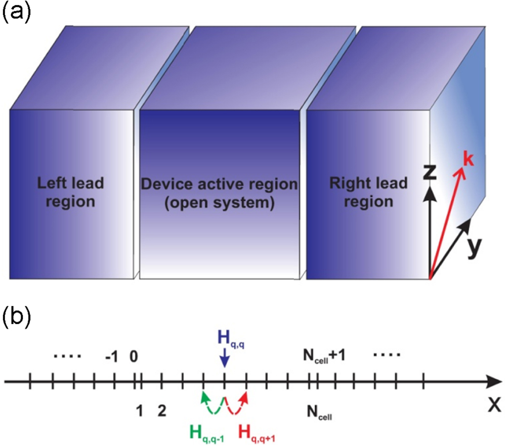
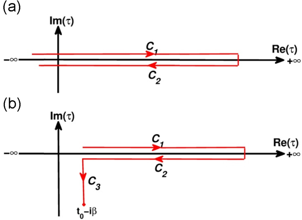
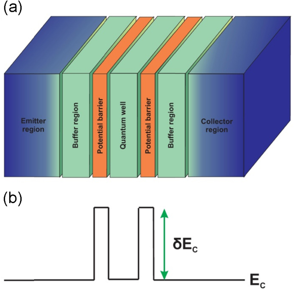
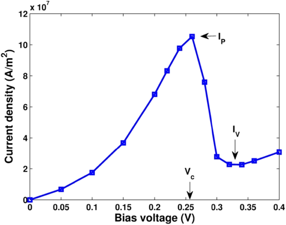
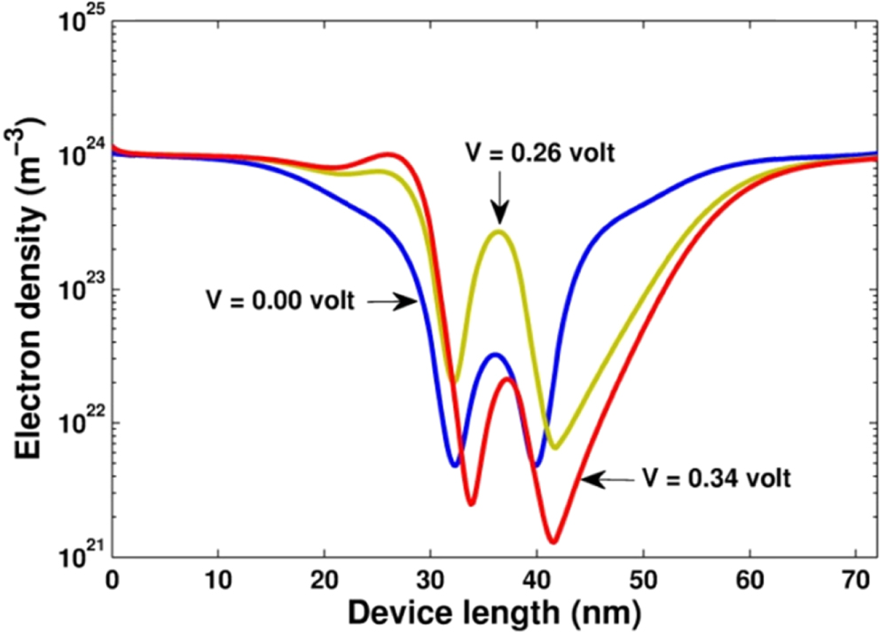
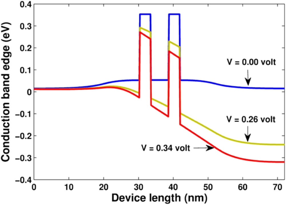
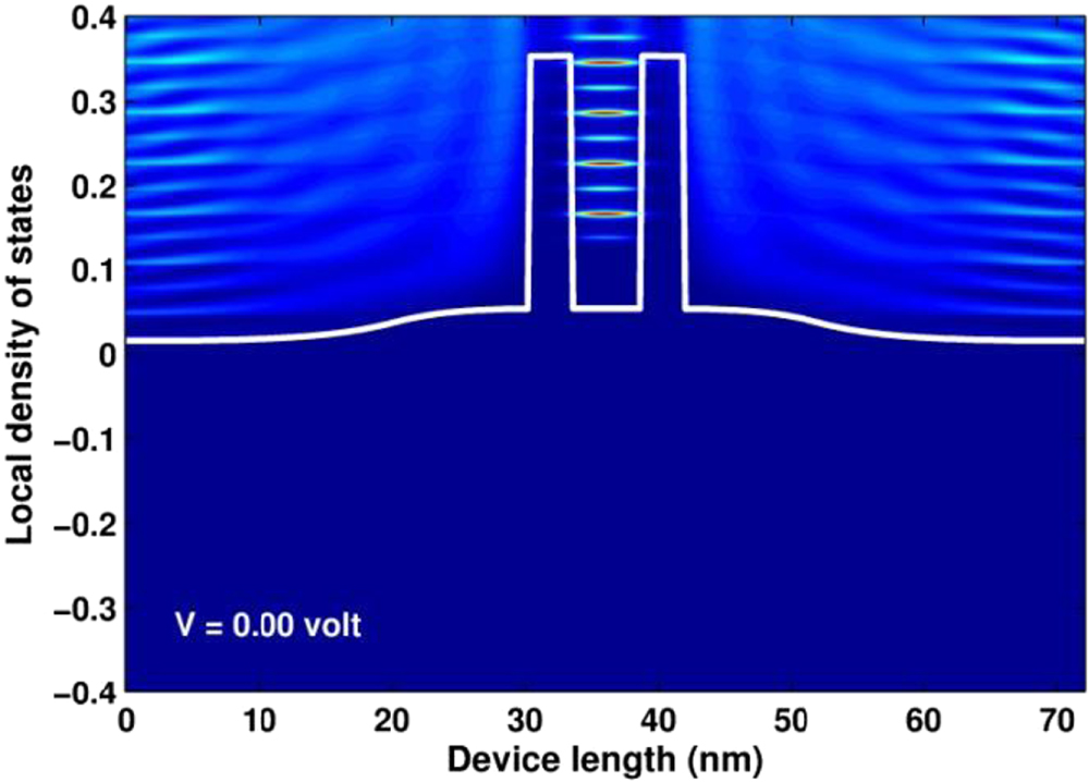
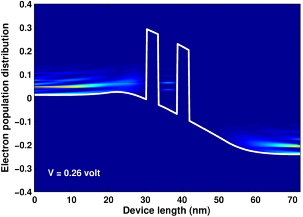
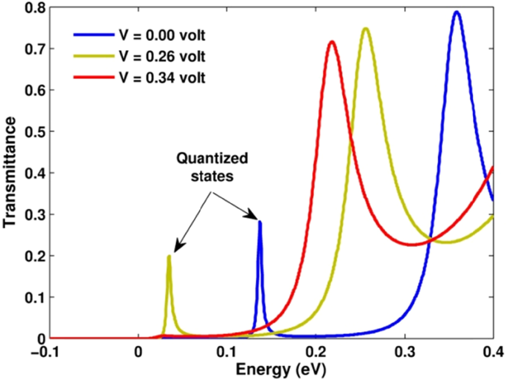
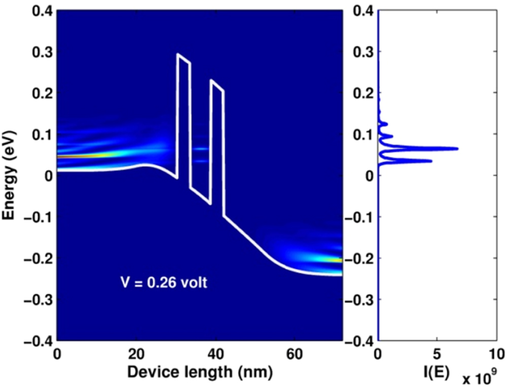
Similarly, the expressions for the function $I_{3}^{a}(t,t\prime )$ read:

$$\begin{eqnarray}&&\begin{array}{lllllllllllllll} I_{3}^{a}(t,t\prime )={{A}^{a}}(t,t\prime ){{B}^{<}}(t\prime ,t) \\ \quad \quad \quad +{{A}^{<}}(t,t\prime ){{B}^{r}}(t\prime ,t)+{{A}^{a}}(t,t\prime ){{B}^{a}}(t\prime ,t) \\ \end{array}\end{eqnarray} \tag{ B.27 }$$

$$\begin{eqnarray}&&\begin{array}{lllllllllllllll} ={{A}^{a}}(t,t\prime ){{B}^{>}}(t\prime ,t)+{{A}^{>}}(t,t\prime ){{B}^{r}}(t\prime ,t) \\ \quad +{{A}^{r}}(t,t\prime ){{B}^{r}}(t\prime ,t) \\ \end{array}\end{eqnarray} \tag{ B.28 }$$

$$\begin{eqnarray}&&\begin{array}{lllllllllllllll} ={{A}^{a}}(t,t\prime ){{B}^{>}}(t\prime ,t)+{{A}^{<}}(t,t\prime ){{B}^{r}}(t\prime ,t) \\ \quad +{{A}^{a}}(t,t\prime ){{B}^{r}}(t\prime ,t) \\ \end{array}\end{eqnarray} \tag{ B.29 }$$

Finally, all the derived results proved above are summarized into table B1, which is usually called the Langreth theorem [9].

Table B1.  Langreth's theorem for the continuum limit rules.

Time-contour	Real-time
$\begin{array}{lllllllllllllll} I_{1}^{\mathcal{C}}(\tau ,\tau \prime ) \\ \quad =\int \mathcal{C} {\mbox{d}}{{\tau }_{1}}{{A}^{\mathcal{C}}}(\tau ,{{\tau }_{1}}){{B}^{\mathcal{C}}}({{\tau }_{1}},\tau \prime ) \\ \end{array}$	$I_{1}^{\lessgtr }(t,t\prime )=\mathop \int \nolimits_-\infty ^\infty {\mbox{d}}{{t}_{1}}[{{A}^{r}}(t,{{t}_{1}}){{B}^{\lessgtr }}({{t}_{1}},t\prime )+{{A}^{\lessgtr }}(t,{{t}_{1}}){{B}^{a}}({{t}_{1}},t\prime )]$
	$I_{1}^{r(a)}(t,t\prime )=\mathop \int \nolimits_-\infty ^+\infty {\mbox{d}}{{t}_{1}}{{A}^{r(a)}}(t,{{t}_{1}}){{B}^{r(a)}}({{t}_{1}},t\prime )$
$I_{2}^{\mathcal{C}}(\tau ,\tau \prime )={{A}^{\mathcal{C}}}(\tau ,\tau \prime ){{B}^{\mathcal{C}}}(\tau ,\tau \prime )$	$I_{2}^{\lessgtr }(t,t\prime )={{A}^{\lessgtr }}(t,t\prime ){{B}^{\lessgtr }}(t,t\prime )$
	$I_{2}^{r(a)}(t,t\prime )={{A}^{r(a)}}(t,t\prime ){{B}^{<}}(t,t\prime )+{{A}^{<}}(t,t\prime ){{B}^{r(a)}}(t,t\prime )+$
	${{A}^{r(a)}}(t,t\prime ){{B}^{r(a)}}(t,t\prime )$
	$={{A}^{r(a)}}(t,t\prime ){{B}^{>}}(t,t\prime )+{{A}^{>}}(t,t\prime ){{B}^{r(a)}}(t,t\prime )-$
	${{A}^{r(a)}}(t,t\prime ){{B}^{r(a)}}(t,t\prime )$
$I_{3}^{\mathcal{C}}(\tau ,\tau \prime )={{A}^{\mathcal{C}}}(\tau ,\tau \prime ){{B}^{\mathcal{C}}}(\tau \prime ,\tau )$	$I_{3}^{\lessgtr }(t,t\prime )={{A}^{\lessgtr }}(t,t\prime ){{B}^{\lessgtr }}(t\prime ,t)$
	$I_{3}^{r(a)}(t,t\prime )={{A}^{r(a)}}(t,t\prime ){{B}^{<}}(t,t\prime )+{{A}^{<}}(t,t\prime ){{B}^{a(r)}}(t,t\prime )+$
	$\quad {{A}^{r(a)}}(t,t\prime ){{B}^{r(a)}}(t,t\prime )$
	$\quad ={{A}^{r(a)}}(t,t\prime ){{B}^{>}}(t,t\prime )+{{A}^{>}}(t,t\prime ){{B}^{a(r)}}(t,t\prime )+$
	$\quad {{A}^{a(r)}}(t,t\prime ){{B}^{a(r)}}(t,t\prime )$
	$\quad ={{A}^{r(a)}}(t,t\prime ){{B}^{>}}(t,t\prime )+{{A}^{<}}(t,t\prime ){{B}^{r(a)}}(t,t\prime )+$
	$\quad {{A}^{r(a)}}(t,t\prime ){{B}^{a(r)}}(t,t\prime )$

The hopping integrals in a many-body Hamiltonian is in general takes the form

$$\begin{eqnarray}&&{{H}_{\nu ,\mu }}=\int {\mbox{d}}{\boldsymbol{r}} \varphi _{\nu }^{*}({\boldsymbol{r}} )\mathcal{K}(\mathop{{\boldsymbol{p}} }\limits^{\hat}){{\varphi }_{\mu }}({\boldsymbol{r}} )\end{eqnarray} \tag{ C.1 }$$

where $\mathcal{K}(\mathop{{\boldsymbol{p}} }\limits^{\hat})$ is the single-particle kinetic operator, an expression of the momentum operator $\mathop{{\boldsymbol{p}} }\limits^{\hat}$. Under a transverse electromagnetic field (assumed to be static), the momentum operator should be changed to the form (the Peierls substitution):

$$\begin{eqnarray}&&\mathop{{\boldsymbol{p}} }\limits^{\hat}\to \mathop{{\boldsymbol{p}} }\limits^{\hat}\prime =\mathop{{\boldsymbol{p}} }\limits^{\hat}-e{\mathbf{A}}({\mathbf{r}})\end{eqnarray} \tag{ C.2 }$$

where ${\mathbf{A}}({\mathbf{r}})$ is the vector potential describing the electromagnetic field, and $e$ the charge of particle. The hopping integrals therefore become dependent on the vector field and can be calculated by replacing $\mathcal{K}\left( \mathop{{\boldsymbol{p}} }\limits^{\hat} \right)$ by the one $\mathcal{K}\left[ \mathop{{\boldsymbol{p}} }\limits^{\hat}-e{\mathbf{A}}\left( {\mathbf{r}} \right) \right]$. However, we know that the system must be invariant under the gauge transformation:

$$\begin{eqnarray}&&{\mathbf{A}}({\mathbf{r}})\to {\mathbf{A}}\prime ({\mathbf{r}})={\mathbf{A}}({\mathbf{r}})-\nabla \theta ({\mathbf{r}})\end{eqnarray} \tag{ C.3 }$$

$$\begin{eqnarray}&&{{\phi }_{\nu }}({\mathbf{r}})\to {{\phi }_{\nu \prime }}({\mathbf{r}})={{{\mbox{e}}}^{-i\frac{e}{\hbar }\theta (r)}}{{\phi }_{\nu }}({\mathbf{r}})\end{eqnarray} \tag{ C.4 }$$

Accordingly, if we require that ${\boldsymbol{A}} \prime ({\mathbf{r}})=0$, then the scalar function $\theta ({\mathbf{r}})$ will be determined through the vector potential A(r) by the following path-integral

$$\begin{eqnarray}&&\theta ({\mathbf{r}})=\mathop \int \limits_\mathcal{C}(O,r) {\mbox{d}}{\mathbf{s}}\cdot {\mathbf{A}}[{\mathbf{s}}({\mathbf{r}})]\end{eqnarray} \tag{ C.5 }$$

where ${\mbox{d}}{\mathbf{s}}$ is a differential element of a path $\mathcal{C}$ connecting the origin point $O$ and the other at the position ${\mathbf{r}}.$

In the case that the basis functions ${{\phi }_{\nu }}({\mathbf{r}})$ are the Wannier's ones, i.e., ${{\phi }_{\nu }}({\mathbf{r}})={{\omega }_{\alpha }}({\mathbf{r}}-{{{\mathbf{R}}}_{i}})$, we can make the approximation

$$\begin{eqnarray}&&\omega {{\prime }_{\alpha }}({\mathbf{r}}-{{{\mathbf{R}}}_{i}})\simeq {{{\mbox{e}}}^{i\theta ({{{\mathbf{R}}}_{i}})}}{{\omega }_{\alpha }}({\mathbf{r}}-{{{\mathbf{R}}}_{i}})\end{eqnarray} \tag{ C.6 }$$

Accordingly, the hopping integrals ${{H}_{\nu ,\mu }}[{\mathbf{A}}]$ becomes

$$\begin{eqnarray}&&\begin{array}{lllllllllllllll} {{H}_{\alpha ,i;\beta ,j}}[{\mathbf{A}}]\simeq {{{\mbox{e}}}^{i\frac{e}{\hbar }{{\theta }_{ij}}}}\int {\mbox{d}}{\mathbf{r}}\omega _{\alpha }^{*}({\mathbf{r}}-{{{\mathbf{R}}}_{i}}) \\ \quad \quad \quad \times \mathcal{K}({\mathbf{p}}){{\omega }_{\beta }}({\mathbf{r}}-{{{\mathbf{R}}}_{j}})={{{\mbox{e}}}^{i\frac{e}{\hbar }{{\theta }_{ij}}}}{{H}_{\alpha ,i;\beta ,j}} \\ \end{array}\end{eqnarray} \tag{ C.7 }$$

where

$$\begin{eqnarray}&&\begin{array}{lllllllllllllll} {{\theta }_{ij}}=\theta ({{{\mathbf{R}}}_{i}})-\theta ({{{\mathbf{R}}}_{j}})=\mathop \int \limits_\mathcal{C}({{R}_{j}},{{R}_{i}}) {\mbox{d}}{\mathbf{s}}\cdot {\mathbf{A}}[{\mathbf{s}}] \\ \quad \quad \simeq {{{\mathbf{R}}}_{ij}}\cdot \mathop \int \limits_0^1 {\mbox{d}}\xi {\mathbf{A}}({{{\mathbf{R}}}_{j}}+\xi .{{{\mathbf{R}}}_{ij}}) \\ \end{array}\end{eqnarray} \tag{ C.8 }$$

where ${{{\mathbf{R}}}_{ij}}={{{\mathbf{R}}}_{i}}-{{{\mathbf{R}}}_{j}}.$