


ABSTRACT
While computing an improved near-Earth object (NEO) steady-state orbital distribution model, we discovered in the numerical integrations the unexpected production of retrograde orbits for asteroids that had originally exited from the accepted main-belt source regions. Our model indicates that ∼0.1% (a factor of two uncertainty) of the steady-state NEO population (perihelion q < 1.3 AU) is on retrograde orbits. These rare outcomes typically happen when asteroid orbits flip to a retrograde configuration while in the 3:1 mean-motion resonance with Jupiter and then live for ∼0.001 to 100 Myr. The model predicts, given the estimated near-Earth asteroid (NEA) population, that a few retrograde 0.1–1 km NEAs should exist. Currently, there are two known MPC NEOs with asteroidal designations on retrograde orbits which we therefore claim could be escaped asteroids instead of devolatilized comets. This retrograde NEA population may also answer a long-standing question in the meteoritical literature regarding the origin of high-strength, high-velocity meteoroids on retrograde orbits.
Export citation and abstract BibTeX RIS
1. INTRODUCTION
We computed a new near-Earth object (NEO) orbital distribution model (Greenstreet et al. 2012) in order to optimize the NEO detection pointing strategy for Canada's NEOSSat (Near-Earth Object Surveillance Satellite), set to launch in mid 2012. Large-scale numerical integrations of particle histories for asteroids leaving the main asteroid belt were used to calculate the steady-state orbital distribution of perihelion distance q < 1.3 AU NEOs. Upon analyzing the numerical integrations, we discovered the surprising production of retrograde orbits from main-belt asteroidal sources, that is, asteroids which orbit "backward" around the Sun. The transfer of asteroids to such orbits has not been previously discussed in the literature. In this Letter, we will first discuss the integration methods used to compute the new NEO orbital distribution model (Greenstreet et al. 2012) before investigating the typical dynamical evolution of these retrograde near-Earth asteroids (NEAs) along with the completeness of the retrograde population. The origin of two known retrograde NEAs as well as the origin of high-strength, high-velocity meteoroids on retrograde orbits will then be connected to the production of retrograde NEAs from main-belt asteroidal sources.
2. INTEGRATION METHODS
The appearance of these retrograde orbits led us to ensure this was not a numerical artifact and to attempt to understand why this behavior had not been reported before.
The new model (Greenstreet et al. 2012) was constructed using the integration algorithm SWIFT-RMVS4, which is an improvement of the algorithm described in Levison & Duncan (1994). This variant provides more accurate and repeatable integrations of the massive planets by preventing time step variations needed to resolve the test particle close encounters from affecting the planetary motion (at the level of the scheme's truncation error). The base RMVS4 time step (when particles are not suffering close encounters) was set to be very small, four hours, in order to produce an accurate integration that correctly resolves even the highest-speed (∼70 km s−1) encounters with all the terrestrial planets; the integrator adaptively reduces this time step to as little as 10 minutes when deep planetary encounters occur. Previous integrations in NEA science often used 3.5 or 7 day base time steps, also subdivided by a factor of 30 upon close encounters. Because the RMVS integrator is second-order accurate in the perturbations, our integration is roughly (3.5/0.17)2 = 425 times as accurate in terms of truncation error than many previous integrations. We believe our integration to be the most accurate long-duration NEA integration yet performed. Although we are unable to easily determine its importance, we also remark that the small time step ensures that close encounters are correctly detected by the integration and that a particle's integration is "slowed down" to correctly resolve the encounter. It is difficult to ascertain what effect a too large time step would have, but it is plausible that incorrectly resolved close encounters would kick high-e and high-i particles to Jupiter-crossing orbits and remove them from the integration prematurely. For example, there exist i > 50° Apollo orbits with e > 0.8 and a ≃ 2 AU; asteroids on such orbits encounter Venus with speeds of >35 km s−1 and thus travel >10 venusian Hill spheres in a single 3.5 day time step, which can result in the integrator incorrectly resolving the close encounter (Dones et al. 1999).
It is not clear that our greater short-term accuracy is important to the retrograde transition in any case, because on the much smaller timescales it takes for particles to transition to retrograde orbits planetary close encounters seem not to be significant. Nearly all of the transitions to retrograde occur in a smooth fashion and relatively quickly (only tens of thousands of years), rendering the higher accuracy of our integration irrelevant as even a 3.5 day time step should correctly incorporate distant planetary perturbations (with close encounters with Earth and Venus being demonstrably unimportant due to the observed lack of sudden orbital element changes). We tested the independence of our results by reintegrating a subsample of our simulations with a different planet set (Venus through Neptune rather than Mercury through Saturn) and the previous generation integrator RMVS3 (more heavily tested) and found no statistically significant differences in the retrograde production mechanism or lifetimes.
This leads one to the question of why the previous Bottke et al. (2002) simulations did not report the production of retrograde orbits from main-belt sources in their previous model. The appearance of these particles in our integrations but not in the previous Bottke et al. (2002) integrations may be due to a variety of factors. The previous, larger time step study (Bottke et al. 2002) may potentially have been removing test particles prematurely via incorrectly resolving close encounters as mentioned above, incorrectly moving particles to Jupiter-crossing orbits and thus cutting off the evolution before the retrograde state could be reached. Second, we have integrated roughly seven times as many particles as previous groups, and this is a rare end state; this is compounded by the fact that the majority of the retrograde residence time is in a minority of long-lived retrograde particles. Third, there is a chance Bottke et al. (2002) produced NEAs on retrograde orbits in their integrations and simply binned them away by forcing these few, rare objects into their 85° < i < 90° bin. Lastly, upon further analysis of our recomputation of the Bottke et al. (2002) integrations (Greenstreet et al. 2012), we observed two example test particles which each flip to retrograde orbits roughly 2 Myr into their lifetimes and live for only ∼300 and ∼900 years post flip. These two extremely short-lived, rare test particles may not have been detected without the higher frequency (300 year) orbital output used in the Greenstreet et al. (2012) model.
3. TYPICAL RETROGRADE NEAS
The production of retrograde orbits coming from asteroidal sources has not been discussed in the literature and was thus surprising. We find that the retrograde population accounts for ∼0.1% (within a factor of two) of the steady-state NEO population (q < 1.3 AU); this fraction is estimated via the complexities of combining the steady-state orbital element distribution of the various asteroidal sources to produce a so-called residence time probability distribution. This distribution for the retrograde NEA population can be found in Greenstreet et al. (2012) and is not reproduced here due to length. The focus of Greenstreet et al. (2012) was to highlight the improvements of the new NEO orbital distribution model from the previous model computed by Bottke et al. (2002). In this Letter, we present a more detailed analysis of the evolutionary paths which lead to the retrograde state and compare the typical retrograde NEA evolution seen in the numerical integrations with the current orbits of known retrograde asteroidal objects and the meteorite record.
After leaving their asteroidal source regions, the typical orbital path for objects which become retrograde is a random walk in semimajor axis a due to planetary close encounters. Some evolve to a < 2 AU and spend many Myr in this state before returning to a larger semimajor axis (Gladman et al. 1997). Often the orbital inclination i rises above 30° during the random walk before the particle returns to a > 2 AU.
The majority of the asteroids which eventually become retrograde find their way into the 3:1 mean-motion resonance with Jupiter after migrating out of any asteroidal source region. Figure 1 shows the logarithm of the amount of time (in Myr) particles live after they become retrograde versus their semimajor axis at the instant their orbits tilt past i = 90°. As can be seen in Figure 1, the great majority of the asteroids that become retrograde do so while in the 3:1 resonance (near a = 2.5 AU). Kozai oscillations (Kozai 1962) inside the resonance are observed to bring the particle's inclination to nearly 80°. It is clear that Kozai alone does not result in the inclination passing through 90°, because only a tiny fraction (if any) become retrograde outside a resonance even if very high-i's are reached. A dynamical phenomenon in the resonance then causes the particle's inclination to make a smooth transition through 90°; the detailed nature of this mechanism is still unclear. However, the smooth evolution of all particle orbital elements during the transition to a retrograde orbit rules out planetary close encounters as the mechanism causing the flip.
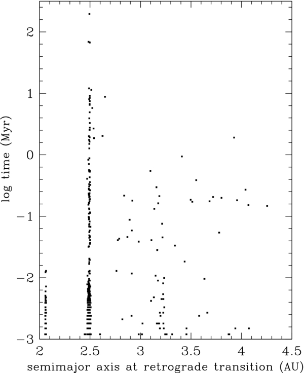
Figure 1. Logarithm of the amount of time (in Myr) particles live after they become retrograde vs. their semimajor axis at the instant they flip to a retrograde state. The vast majority of particles become retrograde while in the 3:1 resonance (near a = 2.5 AU) although other resonant semimajor axes are obvious.
Download figure:
Standard image High-resolution imageIf the retrograde particle stays in the resonance, then it can terminate almost immediately (as little as hundreds of years later) when the resonance pushes the high-e particle into the Sun. Roughly 98% of the retrograde NEAs are eliminated from the integrations because they reach perihelia distances lying inside the Sun, a common fate for resonant asteroids (Farinella et al. 1994). The remaining are either thrown out of the solar system, most often by Jupiter, or suffer planetary collisions. The median lifetime once NEAs become retrograde is only ∼3000 years (Greenstreet et al. 2012), but if kicked out of the resonance due to a planetary close encounter, then the integrations show examples of retrograde asteroids living tens or even hundreds of millions of years.
3.1. Sample Retrograde Production
Figure 2 shows an example of the orbital history of an NEA from our numerical integrations which emerges from the main-belt via the ν6 secular resonance, which is a common mechanism by which asteroids reach planet-crossing space (Gladman et al. 1997; Bottke et al. 2002). This particle gets kicked out of the resonance and random walks in a due to planetary close encounters for most of its lifetime as an Apollo-class NEA. It begins to experience Kozai oscillations in e and i starting at t ∼ 10 Myr, reaching inclinations of up to 75°. Near 70 Myr, the particle has an Earth close encounter which puts it on an orbit near the 3:1 resonance and upon being perturbed into the 3:1 it flips to a retrograde state at t ∼ 72 Myr. It then survives in the retrograde state another 3 Myr before colliding with the Sun. A more detailed analysis of the epoch around the flip (Figure 3) proves that the particle enters the 3:1 resonance. The libration of the 3:1 resonant argument around 180° indicates the importance of the 3:1 resonance at the time of the flip.

Figure 2. a, e, i history from our NEO model integrations of an asteroid which becomes a retrograde NEA. This particle originates in the ν6 secular resonance with low e and i. After a ∼70 Myr sojourn as a high-i Apollo, it flips to a retrograde state crossing i = 90° = 1.57 rad (detail in Figure 3) and lives for another ∼3 Myr before colliding with the Sun.
Download figure:
Standard image High-resolution image
Figure 3. Orbital history of the particle shown in Figure 2 around the time of its flip to a retrograde orbit. Kozai oscillations in e and i are evident from their anti-coupled oscillations and the argument of pericenter librating around 270° from ∼72.1 Myr to ∼72.2 Myr. The 3:1 resonant argument switches from circulating to librating around 180° at ∼72.3 Myr just before the particle flips to a retrograde state.
Download figure:
Standard image High-resolution imageThe longest-lived retrograde particle found in the integrations spends ∼98% of its lifetime in a retrograde state. Starting in the 3:1 resonance, the particle's orbit flips ∼5 Myr into its ∼210 Myr lifetime, having remained in the 3:1 resonance up to that time. About 15 Myr after becoming retrograde, it gets kicked out of the resonance by a planetary close encounter and then random walks to a near ∼2 AU for ∼195 Myr before colliding with the Sun. As shown in Figure 1, although the majority of the NEAs which become retrograde do so while in the 3:1 resonance, the longest-lived retrograde NEAs do not remain in the resonance.
3.2. Completeness of Retrograde Population
We estimate that ∼0.1% (within a factor of two) of the steady-state NEA population is on retrograde orbits. Given the estimate that there are ∼1000 NEOs with H < 18 (D > 1 km) (Bottke et al. 2002; Stuart 2001; Mainzer et al. 2011), of the order of one retrograde NEA of this size should exist at any time. Because NEAs reaching retrograde orbits often visit low perihelion orbits during their evolution then, perhaps like comets (Reach et al. 2009), thermal driven breakup could decrease (if catastrophic) or increase (if many new smaller fragments are produced) this number estimate. In contrast, given that there are ∼7000 known NEAs with H < 23, one might expect more to be known, but this neglects detection biases. The high-e, high-i NEOs are the most incomplete portion of the overall NEO population. The fact that the two known retrograde H < 18 NEAs were only discovered in the last five years (near the end of completing the H < 18 population) proves that these hard-to-find NEOs constitute the most incomplete portion of the NEO population. The incompleteness increases even more for smaller objects.
The Greenstreet et al. (2012) NEO orbital distribution model can be represented as three one-dimensional histograms normalized to the NEOWISE estimate of ∼19,500 NEOs with 18 < H < 23 (Mainzer et al. 2011) and compared to the distributions of already detected NEOs with 18 < H < 23 as seen in Figure 4.

Figure 4. NEO orbital distribution for NEOs with 18 < H < 23 normalized to ∼19,500 NEOs and compared to the 3486 known NEOs with 18 < H < 23 along with the observational completeness for NEOs with 18 < H < 23.
Download figure:
Standard image High-resolution image
Figure 4 expresses the observational completeness of the 18 < H < 23 NEO population as a fraction. Our ∼0.1% estimate for the retrograde NEO population indicates that there should be ≈ twenty 18 < H < 23 NEAs on retrograde orbits. However, the retrograde population at this size are on orbits which are observationally difficult to find; Figure 4 illustrates that as e and i rise, observational completeness plummets rapidly to zero. We thus expect that more retrograde NEAs will be discovered in the near future as the completeness increases for this part of the NEO population.
4. TWO KNOWN RETROGRADE NEAs
There are currently two known retrograde NEAs: 2007 VA85 (a = 4.23 AU, e = 0.74, i = 131 8) and 2009 HC82 (a = 2.53 AU, e = 0.81, i = 1545), which were found by LINEAR and the Catalina Sky Survey, respectively. The Catalina team has recently carefully examined their available imaging of both objects for any evidence of a coma and have found none. It is thus possible that these objects are asteroids that have become NEAs and found their way to i > 90° orbits rather than retrograde devolatilized comets. We do find examples of particles which exit a resonance after flipping beyond 3 AU (Figure 1) and then migrate to larger a; 2007 VA85 has a = 4.23 AU. However, 2007 VA85's current orbital nodes are outside of Jupiter's orbit, so a past close encounter with Jupiter to put it on its current orbit is possible and it may be of cometary origin.
We performed two independent sets of integrations (one using SWIFT-RMVS4 and one with a Bulirsch-Stoer integrator) of the best-fit orbit for each of 2007 VA85 and 2009 HC82 for 1 Myr. 2007 VA85 was terminated by being pushed into the Sun at 0.74 Myr in one integration and was thrown out of the solar system at 0.53 Myr in the other. In both cases, 2007 VA85 migrates to larger a outside Jupiter's orbit. In addition to the best-fit orbit for 2007 VA85, 2000 initial conditions which map the volume in phase space containing 99.9% of the total probability mass (Granvik et al. 2009) for 2007 VA85 were integrated for 1 Myr. About 51% of the clones were pushed into the Sun, ∼37% were thrown out of the solar system, ∼0.5% collided with Jupiter, and ∼11% were still alive after 1 Myr. About 61% of the remaining clones were no longer NEAs (q > 1.3 AU) and had migrated out past Jupiter (a > aJupiter).
2009 HC82, on the other hand, is on an orbit very near the 3:1 resonance (where it most likely flipped) for the entirety of both independent 1 Myr integrations of the best-fit orbit. This behavior is exactly like the typical steady-state retrograde NEA evolution we discovered. Integrations of 2009 HC82's nominal orbit show it to not be currently in the 3:1 resonance. However, our model shows that the long-lived (and thus most likely to be observed) NEAs are those which no longer reside in the resonance. In addition to the best-fit orbit integrations for 2009 HC82, a set of 1458 clones were integrated for 3 Myr. At the end of the 3 Myr integration, ∼51% became Sun-grazers, ∼0.5% were terminated due to planetary collisions, and ∼48% were still alive. Of the 2009 HC82 clones still alive, ∼92% were still near their initial conditions (a ≃ 2.5 AU, q < 1.3 AU), again similar to our expectation.
The dominant evolution for the 2009 HC82 clones is to bounce around near the 3:1 resonance for the duration of the 3 Myr integration, while the 2007 VA85 clones dominantly hit the Sun (or are ejected), where the small percentage still alive at 1 Myr have mostly migrated out past Jupiter and out of NEA space. We therefore think it most likely that 2007 VA85 is a devolatilized comet nucleus; one expects there to be ∼40 multi-km devolatilized Halley-type comet (HTC) nuclei with a < aJupiter (Levison & Duncan 1997; Levison et al. 2006).
5. ESTIMATED EXTINCT COMET POPULATION
A possible production mechanism for an activity-free retrograde NEO is to have a retrograde HTC reach a q < 1.3 AU orbit and have its surface volatiles depleted during numerous perihelion passages, but this is expected to be a rare occurrence. To determine the number of devolatilized HTCs which would exist in a steady-state on orbits with a < 5.2 AU and q < 1.3 AU, we scaled the HTC population model of Levison et al. (2006). Levison et al. (2006) peg the number of active HTCs with D > 10 km and q < 1 AU to be four since this population is believed to be observationally complete. Their Figure 5 shows that ≃60% of the q < 1.3 AU population has q < 1 AU which leads to 4/0.6 ≈ 7 HTCs with D > 10 km and q < 1.3 AU. Also from Figure 5 of Levison et al. (2006), only ∼3% of the q < 1.3 AU HTCs have a < 5.2 AU. This means that the number of HTCs NHTC (D > 10 km, q < 1.3 AU, a < 5.2 AU) ≈ 0.03 × 7 ∼ 0.2. In order to obtain the number of even smaller D > 1 km HTCs on such orbits, the slope α of the logarithmic absolute H-magnitude distribution is needed. Kuiper Belt objects of comparable sizes have α ∼ 0.35 (Fraser 2010). For α = 0.35, because ΔH = 5, NHTC (D > 1 km) = NHTC (D > 10 km) × 101.75 ∼ 10, which is for active HTCs. Figure 11 from Levison & Duncan (1997) shows that for Jupiter-family comets, the favored fade time is ∼104 years and the ratio of extinct to active comets is ∼4. This results in an estimate of ∼10 × 4 ∼ 40 devolatilized HTC nuclei with a < aJupiter at any time. Cometary splitting (Reach et al. 2009) could alter this estimate, but the existence of one or more D > 1 km HTCs, like 2007 VA85, interior to Jupiter is likely. As a final note, the Levison et al. (2006) simulations show that HTCs do not reach a ≈ 2.5 AU, so such an origin for 2009 HC82 seems implausible.
6. HIGH-STRENGTH, HIGH-VELOCITY METEOROIDS ON RETROGRADE ORBITS
The production of retrograde orbits from main-belt asteroidal sources also resolves an outstanding question on the origin of high-strength, high-velocity meteoroids on retrograde orbits. The existence of strongly differentiated material on very high entry-speed orbits (which must be retrograde) has been known since the 1970s (Harvey 1974) and more recent meteor surveys have succeeded in precisely measuring the pre-atmospheric orbits of high-strength meteoroids from retrograde heliocentric orbits (Borovička et al. 2005). The uncomfortable explanation to date for the origin of these high-strength, high-velocity retrograde meteoroids has been cometary (Borovička et al. 2005), but the puzzle existed as to how macroscopic solid rocky components could be on "cometary" orbits. It had been suggested that comets may have internal inhomogeneity which would account for this population of high-strength retrograde meteoroids (Borovička et al. 2005), but little discussion of this appears in the literature. We propose the simpler explanation that these meteoroids are derived from main-belt asteroidal sources. In this scenario, larger (0.01–1 km) NEAs are transferred to long-lived retrograde orbits near (but not in) main-belt resonances and then serve as targets. The collisional production of fragments off these retrograde NEAs would produce smaller retrograde debris on orbits similar to these parent bodies and this debris would then produce the observed high-strength retrograde meteoroids. This explains both the high-velocity, retrograde orbits as well as the high-strength of these meteoroids better than the ad hoc cometary source hypothesis.
S. Greenstreet, B. Gladman, and H. Ngo acknowledge support from the Natural Sciences and Engineering Research Council and the Canadian Space Agency. M. Granvik was supported by the Academy of Finland grant 137853. S. Larson was supported by NASA. We acknowledge CSC–IT Center for Science Ltd. for the allocation of computational resources. This research has been enabled by the use of Compute/Calcul Canada computing resources provided by WestGrid and the SciNet HPC Consortium.