

Abstract
Compressed sensing applied to optical microscopy enables imaging with a number of measurements below the Nyquist criterion. The illumination basis selected, often unstructured for randomness considerations, influences the performance of image reconstruction algorithms. Here, we show through modelling based on multimode fiber imaging that an illumination basis composed of a series of uniformly spaced foci provides improved robustness to noise, increased volumetric imaging performance, and greater resilience to external perturbation when compared to a speckle illumination basis. These observations have broad implications for computational super-resolution imaging, endo-microscopy, and post-processing of images acquired with any point-scanning imaging system.
Export citation and abstract BibTeX RIS

Original content from this work may be used under the terms of the Creative Commons Attribution 4.0 license. Any further distribution of this work must maintain attribution to the author(s) and the title of the work, journal citation and DOI.
1. Introduction
Optical microscopes are an indispensable tool in biology due to their ability to reveal sub-cellular structures as well as dynamic processes in living organisms. In most microscopes, the maximal spatial resolution achievable is dictated by the diffraction limit due to the wave nature of light [1]. The advent of super-resolution (SR) microscopy provided spatial resolution capabilities beyond this limit [2]. Methods to obtain images with extended spatial resolution may be broadly divided into two categories: instrumental and computational SR [3]. Instrumental SR involves specific microscope designs, illumination strategies, and fluorescent probes [2]. For example, in structured illumination microscopy, a twofold increase in spatial resolution is achieved primarily through illuminating the sample with a series of harmonic patterns [4].
Computational SR is achieved primarily through image post-processing. Deconvolution and compressed (or compressive) imaging are two of the most common computational SR methods. Deconvolution and compressed imaging are similar in the sense that they both (a) require knowledge of the illumination sequence and (b) involve solving an ill-posed mathematical problem using an iterative algorithm by optimising a cost function (figure 1(a)). Deconvolution aims to apply the inverse filter to the image with the purpose of reversing the effects of the filtering (convolution) operated by the microscope during the imaging process [5, 6]. Compressed imaging employs compressed sensing (CS) algorithms which have the ability to accurately reconstruct signals with a minimum number of measurements [7–11].

Figure 1. Flowcharts. (a) Summary flowchart of computational imaging methods. (b) Modelling flowchart for two-dimensional analysis.
Download figure:
Standard image High-resolution imageCS algorithms are applicable when the signal of interest is highly compressible or sparse in some space, which is the case for many imaging scenarios [12]. The signal sparsity together with knowledge of the sampling enable probing the signal below Nyquist criterion while still performing accurate reconstruction [12]. The reduction in the number of required measurements offers important advantages in terms of imaging speed and reduced light exposure [12]. These advantages have resulted in the development of several microscopy modalities based on compressed imaging [13–21]. It has been shown that CS algorithms are effective when a pseudo-random sensing mechanism is used to collect the signal [8, 9]. The effectiveness of this randomised sensing mechanism influenced its implementation in optical microscopy where a speckle illumination basis is often employed [16–21].
Instrumental and computational SR methods have been demonstrated to be useful in different scenarios. In particular, SR imaging through multimode optical fiber (MMF) has only been demonstrated with two computational methods: first with deconvolution and then with compressed imaging [21, 22]. As mentioned above, compressed imaging commonly employs a sequence of different speckle patterns (speckle illumination basis), while deconvolution typically involves a sequence of foci at different locations (focus illumination basis). However, CS algorithms pose few restrictions on the type of illumination to be used. This observation suggests that a sequence of individual and equidistant foci, such as is used for deconvolution, could serve as the illumination basis for compressed imaging (figure 1(a)). This approach is particularly appealing as this sampling strategy is known for its efficiency and the unbiasedness of the estimators it produces [23], but also because this sampling basis is used by a wide array of microscope modalities, including point-scanning systems.
In the present work, we performed a comparative study to characterise the performance of different computational SR methods. We compared the performance of focus illumination and speckle illumination for compressed imaging (supplementary video 1 and video 2 available online at stacks.iop.org/JOpt/24/065301/mmedia). In particular, we modelled the effect of noise on the quality of the reconstruction, potential for fast volumetric imaging, and the impact of external perturbations.
2. Methods
2.1. Modelling overview
The flowchart in figure 1(b) summarises the modelling sequence implemented for two-dimensional (2D) computational super-resolution imaging based on compressed imaging and deconvolution. First, we generated different illumination bases ill: focus illumination, speckle illumination, and array illumination. Focus illumination consisted in a sequence of single diffraction-limited focus at different lateral positions in the sample, which is equivalent to standard point-scanning imaging (supplementary video 1). Speckle illumination consisted in a sequence of unique speckle-like intensity distribution covering the surface of the image (supplementary video 2). Array illumination consisted in a sequence of multiple diffraction-limited foci at different lateral position in the sample following a structured arrangement (supplementary video 3). All illumination bases were generated by modelling propagation through a MMF. In some cases, perturbations were introduced in the illumination illper in the form of optical aberrations or bending of the fiber. For the latter, it was necessary to calculate new sets of illumination bases. However, illper was equal to ill in most cases.
In parallel, we also generated artificial 2D bead samples (Object A). Then, we generated the noisy signal Sσ . For compressed imaging, each measurement Si in the signal S was calculated by integrating all the elements in the matrix resulting from the element-wise multiplication between A and illper. For deconvolution, A was convolved with a single focus from the focus illumination to generate S. Sσ was generated by adding varying amounts of zero-mean Gaussian white noise with a specified variance σ.
Next, we performed computational super-resolution imaging using CS and deconvolution algorithms. The super-resolution image B was obtained based on two primary inputs: the noisy signal Sσ and the unperturbed illumination ill. In other words, the algorithms had no knowledge of any perturbations, noise level, or ground truth A. Compressed image reconstruction was performed using the basis pursuit algorithm. Deconvolution was performed using a modified Lucy-Richardson (LR) algorithm with total variation regularisation. Finally, the performance of the SR image reconstruction process was assessed quantitatively by comparing the SR image B to the ground truth object A by calculating the correlation coefficient R.
Using the methodology outlined above, the performance of compressed imaging with the different illumination bases and deconvolution was assessed for varying amounts of noise. The use of focus and speckle illumination was also compared for compressed imaging in the presence of perturbation. The three-dimensional (3D) analysis is described in details below.
2.2. Sample generation
Synthetic imaging data was generated by simulating 2D and 3D bead images. The 2D bead images were simulated by producing an array of 2D points at random locations using a salt and pepper noise function with a density of 0.001 on a  null matrix. The beads were then restricted within a given radius from the centre of the image (53 pixels). Finally, the intensity of the beads was randomised following a Gaussian distribution (σ = 0.5) and all beads were given the same diameter using Gaussian filtering (σ = 1.33). A total of 21 2D images were generated and the width, given as the full width at half maximum, of each bead objects was 1.44 µm. Similarly, 3D bead images were simulated by producing an array of 3D points at random locations using a salt and pepper noise function with a density of 0.0015 on a
  null matrix, where Z is the number of axial planes (Z = 60). The beads were then restricted within a radius of 16 pixels from the image centre and between the 8th and 52nd axial planes. Finally, the beads were given the same diameter using Gaussian filtering (σ = 0.93). Five 3D images were generated.
2.3. Modelling 2D illumination
To facilitate the comparison between speckle and focus illumination, a MMF-based endo-microscope system was simulated. This system enabled the generation of both speckles and foci in the sample by giving different shapes to the wavefront entering a straight fiber at the proximal end. The original MATLAB code that was modified for this work can be accessed at [24] and is based on the model described in Plöschner et al [25].
Foci were generated in the sample by first evaluating the transmission matrix using a sequence of proximal foci and then calculating its regularised inversion. A proximal grid of  pixels and a distal grid of
  pixels were used for the simulation. The resulting illumination matrix was then sub-sampled to select 2401 foci uniformly covering the sample over the surface of the core. The focus illumination basis is shown in supplementary video 1.
Speckle patterns were generated in the sample by focusing light at different location of the MMF proximal end. The resulting speckle patterns were determined also by using the transmission matrix. A proximal and distal grid of  pixels were used for speckle simulation. The resulting illumination was then sub-sampled to 2401 illuminations uniformly covering the proximal core area. The speckle illumination basis is shown in supplementary video 2.
For all 2D analyses, light at 532 nm was modelled going through a MMF having a diameter of 50 µm, a numerical aperture of 0.22, and a length of 1 m. Normalisation was applied such that the total intensity was the same for both illumination strategies. For bending, a single fiber segment was considered with a curvature defined by a bending radius  [24].
[24].
2.4. Modelling 2D signal and analysis
For compressed imaging with either illumination basis, the signal was calculated by integrating the matrix resulting from the element-wise multiplication of the 2D illumination and 2D sample for each illumination composing the basis. For deconvolution, the object was convolved with the central focus. For all reconstruction methods, a zero-mean Gaussian white noise with a specified variance σ was superimposed onto the signal when needed. To characterise the quality of the reconstruction process, the correlation coefficient R, the mutual coherence µ, and the error probability  were calculated as described in the supplementary information.
For bending, the signal was calculated by pixel-wise multiplication of the 2D bent illumination and 2D sample for an illumination in the sequence and then integrated. The SR image reconstruction processed was agnostic to the bending and assumed illuminations from an straight fiber. Information regarding the modelling with optical aberrations can be found in the supplementary information.
2.5. Modelling 3D illumination and signal
Analyses for volumetric imaging were implemented for focus illumination only. Distal foci in 3D were created by first generating 2D foci as described in the previous section and then propagating them axially using a defocus function. A proximal grid of  pixels and a distal grid of
  pixels were used for the simulation. The resulting illumination matrix was then sub-sampled by a factor of 2 to select foci uniformly covering the sample over the surface of the core. For all 3D analyses, light at 930 nm was modelled going through a MMF having a diameter of 50 µm, a numerical aperture of 0.37, and a length of 1 m. The signal was calculated by integrating the matrix resulting from the element-wise multiplication of the 3D illumination and 3D sample for each illumination composing the focus illumination basis. The outcome of SR image reconstruction was evaluated by calculating the axial and lateral full width half maximum (FWHM) of beads. The lateral and axial profiles were manually obtained for two randomly selected beads in each of the 3D reconstructions. The FWHM was then calculated by finding the four points neighbouring 50
 of the peak intensity value on each side of the peak and performing a linear interpolation between the two points to determine the positional values of both half maximum [26].
2.6. Super-resolution image reconstruction
For compressed image reconstruction, we used the basis pursuit (BP) algorithm [8] with a maximum number of iterations set to 3000 and a modified calculation of pseudo-inverse calculation for additional precision [27]. More information about the theory of compressed sensing is available elsewhere [7–11]. The augmented Lagrangian and over-relaxation parameters were both set to 1.0. For deconvolution, we used the modified LR algorithm with total variation regularisation [5, 22, 28, 29]. A uniform point-response was assumed across the surface of the fiber, as obtained in the focus illumination basis. The algorithm performed nine iterations, which was empirically determined to provide the best performance.
3. Results
3.1. SR image reconstruction
The performance of the three different SR image reconstruction methods was first compared in the noiseless scenario with the 2D bead data. Figure 2(a) shows an example set including the ground truth object, the diffraction-limited image, and the reconstructed SR images using the BP algorithm with speckle and focus illuminations and using the LR deconvolution algorithm. Extended spatial resolution was achieved with all SR image reconstruction methods when compared to the diffraction-limited image (figure 2(a)). Use of the BP algorithm with any illumination resulted in no visually perceptible difference between the SR image and the ground truth object (figures 2(a) and (b)). When using LR deconvolution, small errors in the reconstruction were visible when tracing line profiles but overall the reconstruction quality was still high, which is expected for a noise-free signal (figure 2(b)).

Figure 2. Computational SR imaging. (a) Example set including the ground truth (Object), the diffraction-limited image (Image), and the reconstructed SR images using the BP algorithm with speckle (BP speckles) and focus illuminations (BP foci) and using the LR deconvolution algorithm (LR deconvolution). Image width: 54.5 µm. (b) Intensity profile of the line shown in (a). (c) Correlation coefficient R between the ground truth and the SR images for different level of sparsity (0.1, 0.01 and 0.001).
Download figure:
Standard image High-resolution imageThe correlation coefficient R between the ground truth object and the SR images was calculated for the analysis to be quantitative. For the original bead density (0.01), R was above 0.998 with the BP algorithm and below 0.997 with the LR deconvolution algorithm in accordance with the above observations. A denser (0.1, 10×) and sparser (0.001, 0.1×) dataset were also generated to assess the effect of sparsity on the quality of the reconstruction. As expected for compressed imaging, R increased with increased sparsity (figure 2(c)). The same dependence was observed for the LR algorithm. However, while both illumination strategies yielded similar R value for all bead densities with the BP algorithm (figure 2(c)), the LR algorithm appeared to be more sensitive to sparsity as exemplified by the much lower R value of 0.9816 ± 0.0016 for the denser objects. In summary, all SR image reconstruction methods were successful when no noise was present in reconstructing images with increased spatial resolution, but use of the BP algorithm provided the optimal results regardless of the chosen illumination pattern. The results from figure 1(c) also confirm that the samples were sufficiently sparse in the spatial domain to meet the sparsity condition of CS algorithm and as such no basis transformation was necessary.
3.2. Noise analysis
Next, the impact of noise for the three different SR image reconstruction methods was assessed by processing the dataset with varying amount of noise. The three methods had strikingly different noise dependence as shown by the graph of R with respect to the ground truth object as a function of noise (figure 3(a)). By fitting a logarithmic logistic function, the 50%-R value, denoted τnoise, was found to be  ,
,  and
and  for the LR deconvolution algorithm, BP algorithm with speckle illumination and BP algorithm with focus illumination, respectively. It is of note that the BP algorithm with focus illumination utilised the same type of illumination but only a fraction of the measurements compared to LR deconvolution, yet outperformed the latter. To explore this result further, the BP algorithm was used to reconstruct SR images with varying noise using the same illumination, including the number of measurements (no compression), as for LR deconvolution (figure 3(a)). A τnoise value of
  was obtained, which is larger than for the LR algorithm on the same data. This observation suggests that CS algorithms might be preferable over LR deconvolution even when there is no data compression.

Figure 3. Compressed imaging with noise. (a) Correlation coefficient R between the reconstructed SR image and the ground truth object as a function of noise for processing with the LR deconvolution algorithm (LR algorithm), BP algorithm with speckle illumination (BP speckles), B.P. algorithm with focus illumination (BP foci), and BP algorithm with focus illumination and without compression (BP foci n.c.). (b) and (c) Example SR images of fluorescent beads reconstructed with the same amount of noise ( ) using (b) the BP algorithm with focus illumination and (c) the BP algorithm with speckle illumination. Image width: 54.5 µm.
Download figure:
Standard image High-resolution imageMore importantly, figure 3(a) shows that, for a given CS algorithm, the robustness to noise will depend on the illumination. Indeed, unlike for the noiseless case, the robustness of the BP reconstruction algorithm to noise was better for focus than speckle illumination, given equivalent data compression (figures 3(b) and (c)). In addition, focus illumination with compression outperformed the no compression case when the total incident power was equal. Together, these results suggest that the structure of the illumination and the efficiency of spatial sampling should both be considered as key factors. The comparative noise analysis between focus and speckle illumination using the BP reconstruction algorithm was repeated on images of extended objects. For this purpose, 21 images of hand-written numbers from the MNIST dataset were processed; no parameters were changed. The τnoise was found to be  and
and  for the BP algorithm with speckle illumination and BP algorithm with focus illumination, respectively (figure 4(a)). This result, further illustrated by example SR images in figures 4(b) and (c), confirms that focus illumination provides more robustness to noise than speckle illumination when used with a CS algorithm, even when applied to more complex images.

Figure 4. Compressed imaging of extended source with noise. (a) Correlation coefficient R between the reconstructed SR image and the ground truth object for extended sources image from the MNIST database as a function of noise for processing with BP algorithm with speckle illumination (BP speckles) and BP algorithm with focus illumination. (b) and (c) Example SR images of extended sources from the MNIST database reconstructed with the same amount of noise ( ) using (b) the BP algorithm with focus illumination and (c) the BP algorithm with speckle illumination. Image width: 54.5 µm.
Download figure:
Standard image High-resolution imageThe source of the dependence on the illumination when processing noisy data with CS algorithms was investigated by using a third type of illumination with the BP algorithm. This third illumination consisted of structured arrays of foci (supplementary video 3). The number of foci per array was varied such that a range of τnoise values, between that of single foci and speckle illuminations, were obtained when processing the data and fitting the logarithmic logistic function (figure 5(a)). The mutual coherence µ was then calculated to quantify the incoherence condition. This condition dictates that a maximally incoherent sampling provides an optimal sampling of the space and, accordingly, a low mutual coherence is preferred for the illumination [12]. In line with this principle and the above observations,  was lower than
  (figure 5(b)). Sampling incoherence is not necessarily the only factor at play in explaining the difference between focus and speckle illuminations because array illumination with 8 or more foci per illumination have a higher µ than speckle illumination, yet their τnoise is higher (figures 5(a) and (b)).
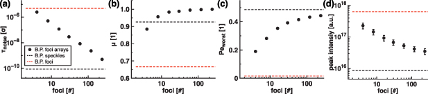
Figure 5. Performance of compressed sensing algorithms as a function of the illumination. The following parameters are plotted against the number of foci in foci array illumination: (a) the 50%-R value from logarithmic logistic regression of the noise analysis τnoise with the BP algorithm, (b) the mutual coherence µ, (c) the higher bound of the error probability  , and (d) the peak intensity of the generated signal. The values of these parameters are also given for focus and speckle illumination.
Download figure:
Standard image High-resolution imageAnother important factor to consider is the probability of making an error during the reconstruction. This probability is dependent on the illumination as well as the object and is not easily calculated. The higher bound of the error probability  serves as a good proxy metric as its calculation is tractable and can be expressed in an object-independent manner for the relative comparison of different illuminations [30]. Figure 5(c) indicates that focus illumination has a lower
  than speckle illumination and that as the number of foci in array illumination increases
  approaches
  . This can be intuitively understood by considering that a fixed amount of noise is added to a decreasing peak signal as the number of foci in the array illumination increases (figure 5(d)). In brief, several factors may contribute to the increased robustness to noise with focus illumination compared to speckle illumination, including improved space sampling and decreased error probability.
3.3. Volumetric imaging
Several approaches have been implemented to achieve 3D compressed imaging with the goal of minimising photo-bleaching and increasing imaging speed [31–33]. One approach for 3D compressed imaging consists of acquiring data at different axial planes with a series of known 3D speckle patterns and then reconstructing a 3D image with a CS algorithm. The robustness to noise would again be improved with focus illumination as the reconstruction does not depend on the image dimensionality. Indeed, the signal is treated as a one-dimensional vector by the CS algorithm, even when objects are 2D and 3D. The computational requirement of this approach scales with the cube of the number of axial planes as the number of required measurements increases linearly and the size of the illumination matrix with the square of the number of axial planes. The entire volume also needs to be sampled, even when capturing a single axial plane is desired.
SR compressed imaging combined with optical sectioning would be a time- and computation-efficient strategy for 3D imaging or for rapidly imaging a single axial plane. Only the axially-restricted illumination pattern in the plane of interest would need to be known and probed for 2D image processing [33]. A 3D image can then be constructed from a series of 2D images, individually processed. We implemented this approach with focused light as it enables the use of two-photon excited fluorescence, which intrinsically provides optical sectioning. An axial-lateral projection shows that optical sectioning can indeed be achieved (figures 6(a) and (b)). Analysis of bead profiles by FWHM measurements indicated that an extended spatial resolution is attained along the lateral dimension ( ) and diffraction-limited performance along the axial dimension (
 ) when compared to the diffraction-limited data (
 ,
,  ) and reference object (
 ,
,  , figures 6(c) and (d)).
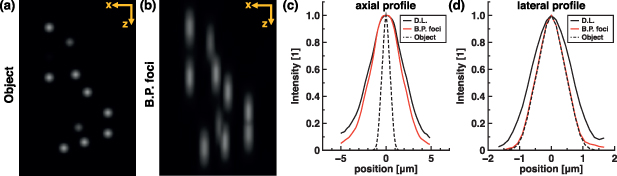
Figure 6. Three-dimensional imaging and compressed sensing. (a) and (b) Example axial (z)-lateral (x) projections of (a) the ground truth object and (b) the associated SR image in which each axial plane was reconstructed independently using focus illumination for multiphoton excitation and the BP algorithm. Image width: 54.5 µm. (c) and (d) Example profiles from a single simulated bead along (c) the axial and (d) lateral directions for the ground truth (Object), the diffraction-limited image (DL), and the SR compressed image (BP foci).
Download figure:
Standard image High-resolution imageIn summary, fast volumetric imaging with extended lateral resolution can be achieved with two-photon excited fluorescence, focused light, a.nd SR CS algorithm.
3.4. Bending and multimode optical fiber
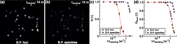
The above analyses are valid for any optical system in which focusing is possible. In this section, we focus on the specific issue of imaging through a bent MMF. For imaging through a MMF, the wavefront entering the proximal end can be shaped such that a focus is formed in the sample [34–36]. Determination of the optimal wavefront requires a calibration, which is only valid for the mechanical state in which the calibration was performed, typically in a straight MMF. If the MMF is bent, the calibration is no longer valid and the focus quality decreases [25, 37, 38]. The same is true for speckle patterns; for a given input, the output will change as the MMF is bent.
The resilience to bending of SR compressed imaging through a MMF was evaluated for speckle and focus illuminations. Illumination changes were simulated with different bending radius  and the signal processed with the expected and known illumination patterns (that of a straight MMF). It was observed that using the BP algorithm with speckle illumination was less resilient to bending then using the same algorithm with focused light (figures 7(a) and (b)). Indeed, the reconstruction quality, as assessed by R with respect to the ground truth, dropped off at a much larger
  for speckle than for focus illumination (figure 7(c)).
Figure 7. Compressed imaging with perturbed illumination. (a) and (b) Example SR images of fluorescent beads reconstructed with the same bending radius ( (m)) using (a) the BP algorithm with focus illumination and (b) the BP algorithm with speckle illumination. Image width: 54.5 µm. (c) Correlation coefficient R between the reconstructed SR image and the ground truth object as a function of
  for processing using the BP algorithm with speckle and focus illuminations. (d) Correlation coefficient
  between the illumination with and without perturbation for both speckle and focus illuminations.
Download figure:
Standard image High-resolution image
Here again the sampling incoherence and error probability may play a role. However, the evolution of the illumination with bending is likely a more important factor. The correlation coefficient between the straight and bent illumination  was therefore calculated as a function of
  (figure 7(d)). The illumination remained more similar with focus than speckle illumination during bending. This difference can be understood as follows: while the intensity distribution changes uniformly across the area illuminated with a speckle pattern with bending, the fraction of light contained in the focus is still much higher than the background outside the focus.
  only partially captures this idea. In sum, the overall illumination changes less rapidly with bending for focused light than for speckles patterns and, as such, focus illumination offers more resilience to bending.
4. Discussion
The performance of compressed imaging depends on the relationship between the sample sparsity and the illumination [11]. In many imaging applications, including fluorescence imaging, the object distribution is sparse in the Cartesian object space [12]. The optimal illumination basis should then be maximally incoherent in this space. We showed that illuminating the sample sequentially with individual and equidistant foci is more efficient, according to the mutual coherence, then using randomly generated speckle patterns. This approach is known as systematic random sampling and is stochastic provided that the origin of the illumination grid is randomly selected [23]. It is well known in stereology that systematic random sampling of the surface of a biological object provides faster convergence toward expected statistical properties than other random sampling configurations. When selecting an illumination basis for compressed imaging, it is also necessary to consider the probability of errors during image reconstruction due to the illumination [30]. We showed that this error is smaller for focus illumination than speckle illumination.
It should be emphasised that the advantages afforded by focus illumination in compressed imaging are valid for any microscope capable of focusing. We illustrated this fact with one-photon and two-photon endo-microscopy with MMF, but the observations can easily be extended to confocal and multiphoton point-scanning systems. In other words, these advantages are properties of the illumination basis. This fact also implies the generalisability of the method to any CS algorithm. We validated this idea by repeating the noise, the optical sectioning, and the bending analyses with a different CS algorithm ( -Dantzig) and were able to draw the same conclusions (see supplementary figure S1).
The sampling ratio, here defined as the number of measurements divided by the number of pixels, was 25% for all 2D analyses. Considering the physical parameters used in the simulations (wavelength, pixel size, numerical aperture, and the number of modes supported by the MMF), a sampling ratio of 25% was sufficient to achieve perfect image reconstruction in the absence of noise (figure 2). This result was expected from the fact that a sampling ratio of 25% here corresponded to a number of measurements equal to the number of modes supported by the MMF. As the sampling ratio is further decreased, insufficient information will be acquired, and the quality of the reconstruction will decrease both for focus and speckle illuminations. Of course, uniform spatial coverage of the entirety of the sample should be maintained and the numerical aperture of the system should thus be chosen accordingly. In other words, it would be desirable to increase the size of the focal volume for focus illumination as the sampling ratio decreases. There might also be benefits in increasing the characteristic speckle size; however, this strategy was not investigated. Other systematic sampling approaches might also provide enhanced performance as compression increases.
The alteration of the illumination pattern with bending is a major challenge for the field of MMF-based endo-microscopy [25, 37, 38]. Many strategies have been proposed to alleviate or correct the effect of bending, including the use of a high numerical aperture, numerical solutions based on knowing the fiber deformation, and sensing the transmission matrix by using distal probes [25, 38–40]. The increased resilience to bending of focus compared to speckle illumination in the context of compressed imaging can be combined with these other strategies to facilitate the deployment of MMF endo-microscopes in applications involving fiber deformation and simultaneously achieving SR computational imaging [20, 21, 41, 42]. However, here again the implications are broader then for MMF alone. Indeed, the fact that focus illumination retains more self-similarity with perturbations then speckle illumination could be beneficial for a broad range of perturbations. We illustrated this fact by analysing the performance of CS algorithm in the presence of optical aberrations because aberrations are frequently encountered in several type of optical microscopes and other high resolution optical imaging systems in which compressed imaging could be deployed [43]. We found that focus illumination was more resilient to aberration than speckle illumination (see supplementary figure S2).
Finally, compressed imaging as a computational SR methods compared favourably to SR deconvolution. This result is particularly interesting given that a grid of foci was employed in both cases but that fewer data points were collected for compressed imaging. This observation suggests that standard imaging data could be post-processed more effectively, in terms of signal-to-noise ratio, by using a CS algorithm even when the sampling is above the Nyquist criterion.
In conclusion, there are several advantages of using focused light over speckle illumination for compressed imaging. Focus illumination provides more robustness to noise, faster volumetric imaging, and increased resilience to perturbation of the illumination. These advantages are directly related to the illumination in a sparse Cartesian object space; they are independent of the specific CS algorithm employed or how the foci are generated. Therefore, we believe that the proposed approach of combining focus illumination and CS algorithm will find broad applicability in many diffraction-limited and SR optical imaging systems.
Data availability statement
All modelling resources are hosted publicly on GitHub (https://github.com/dop-oxford/CIFL). The data that support the findings of this study are openly available at the following URL/DOI: https://github.com/dop-oxford/CIFL.
Acknowledgment
European Research Council (695140); Engineering and Physical Sciences Research Council (EP/R511742/1).