
Abstract
This review provides an insight into the recent developments of photonic crystal (PhC)-based devices for sensing and imaging, with a particular emphasis on biosensors. We focus on two main classes of devices, namely sensors based on PhC cavities and those on guided mode resonances (GMRs). This distinction is able to capture the richness of possibilities that PhCs are able to offer in this space. We present recent examples highlighting applications where PhCs can offer new capabilities, open up new applications or enable improved performance, with a clear emphasis on the different types of structures and photonic functions. We provide a critical comparison between cavity-based devices and GMR devices by highlighting strengths and weaknesses. We also compare PhC technologies and their sensing mechanism to surface plasmon resonance, microring resonators and integrated interferometric sensors.
Export citation and abstract BibTeX RIS

Original content from this work may be used under the terms of the Creative Commons Attribution 3.0 licence. Any further distribution of this work must maintain attribution to the author(s) and the title of the work, journal citation and DOI.
1. Introduction
Photonic sensors continue to be high on the agenda because of the ever-increasing demand for sensing applications in areas such as healthcare, defence, security, environment and food quality control, with a particular emphasis on miniaturised and personalised technologies. According to a market analysis performed by Allied Market Research, the global photonic sensor market is expected to reach an impressive $15.2bn total market revenue by 2020, with Europe being a very strong contributor [1]. A significant slice of this market is represented by photonic biosensors. Correspondingly, research on photonic biosensors has also steadily increased over the years because of the many exciting research challenges they offer. This trend is reflected by the ISI Web of Science, which shows how the number of publications in the area has more than doubled in the last 10 years, with 2.2k papers containing the keyword 'biosensor' published in 2007 and 4.8k in 2017, compared to an annual growth rate in the total number of papers of approximately 3% [2]. A similar trend is observed for 'optical biosensor' papers [3].
The purpose of a biosensor is the detection of biologically-relevant targets such as proteins, DNA, pathogens, cells, bacteria, pollutants, hormones and enzymes. In most cases, their presence and/or concentration in samples such as blood, urine, saliva, sweat or tears can be an early indicator of disease, so that the sensor can be used as a valuable diagnostic tool.
In its general form, a biosensor is a transducer that reports a molecular or biochemical binding event as a physical quantity. In the case of a surface affinity biosensor, the sensing element is a surface covered in a biorecognition molecule such as DNA, proteins, antibodies or particular cell receptors that can selectively bind to targets in the analyte under examination. Depending on the transduction mechanism, biosensors can be classified into electrical, electrochemical, piezoelectric, nanomechanical, acoustic, magnetic or optical.
In our case, the transducing mechanism is optical, meaning that the binding event modulates the interaction with optical radiation in a detectable way. While a comprehensive comparison with other sensing modalities is beyond the scope of this review, we note that some of the key advantages of optical transducers is that they are non-corrosive, they do not suffer from electromagnetic interference and they afford parallel, non-contact readout. Optical biosensors can be further divided into fluorescence-based and label-free devices. Fluorescence is still the most commonly employed configuration, whereby target molecules are labelled with fluorescent tags, such as dyes, whose fluorescence intensity is indicative of the presence of the analyte(s) of interest and its interaction with the dye. Although this scheme can be sufficiently sensitive to detect single molecules, the requirement for fluorescent labelling complicates the procedure, it may distort the measurement and it can interfere with the function of the biomolecules. In the interest of simplicity, here, we focus on label-free optical methods.
The examples of label-free techniques we are considering here all rely on guided-wave optics, whereby light propagates in a waveguide and the evanescent tail of the guided mode interacts with the analyte. Upon binding, the refractive index (RI) at the surface changes, which modulates the phase of the guided mode via the effective index. This change in phase is picked up interferometrically or by placing the mode in a resonant structure and recording the change in resonant wavelength, so the large majority of label-free photonic sensors are RI sensors. Optical absorption may also be used instead, but since most biological targets are phase objects, RI sensing tends to be the preferred option.
A particular photonic structure that can be used for sensing is a photonic crystal (PhC). PhCs consist of a spatially periodic arrangement of dielectric materials. Their operation can be easily understood via their analogy with electrons in a crystalline structure: a PhC does to photons what a semiconductor crystal does to electrons. The analogue of the periodicity of the coulombic potential in a semiconductor is the periodicity of the dielectric constant.
The key characteristic, for a judicious choice of materials and geometry, is the presence of a photonic band gap, namely a range of frequencies that are not allowed to propagate in the structure. The origin of this band gap is the constructive interference of waves reflected at the different dielectric material interfaces. The easiest way to picture this is a distributed Bragg reflector (DBR), namely a periodic stack of alternating dielectric materials of different RI. Such a stack exhibits a band gap when half the wavelength in the material corresponds to the period of the stack. The presence of a band gap can be exploited to create waveguides, micro-cavities, or to enhance nonlinear effects. It is also possible to tailor the interference between leaky modes in order to obtain a desired spectral behaviour: PhCs exquisitely allow us to mould and adapt the flow of light to our needs.
Two main classes of PhC-based sensors will be discussed in this review, namely devices based on (a) PhC cavities and (b) on guided mode resonances (GMRs). We believe that this distinction perfectly reflects the versatility of PhCs and it captures all their relevant aspects and advantages. This paper complements other excellent reviews in this area [4–11] and we will focus on some relevant examples to highlight routes for enhancing performance, underline the differences to related approaches and discuss strengths and weaknesses.
PhC cavities offer a very high degree of spatial confinement, resulting in a very small footprint and the possibility for extreme miniaturisation. This strong localisation comes with a high degree of wavelength selectivity: ultra-high Q factors of up to 107 have been measured [12]. We note that this combination of high spatial with high spectral confinement is unusual in photonics; typically, one thinks of high Q cavities as being large objects and not wavelength-scale. These characteristics make PhC cavities suitable for multiplexing and very localised sensing of biomarkers, cells and bacteria. In terms of sensing properties, the high Q translates into a low limit of detection (LOD), while the small volume translates into very small analyte volumes and the possibility to even measure inside cells, as we will discuss later.
The second model system, i.e. GMR-based devices, exploits in-plane resonant modes which are excited by collimated out of-plane radiation. The ability to couple directly to the resonant modes is a very attractive feature because of the easiness of interfacing with light sources, especially in the context of point-of-care (POC) devices. Furthermore, they are inherently able to spatially resolve the resonance information, so they are also suitable for imaging. However, this ease of interfacing comes at the cost of reduced Q factor and sensitivity compared to the cavity approach.
The paper is organised as follows. Section 2 presents a brief introduction of the physics of PhCs, both for cavities and GMR-based geometries. We then move onto discussing figures of merit used for assessing biosensor performance in section 3. In section 4, PhC cavity sensors are reviewed and compared to SPR devices. A similar comparison is conducted in section 5 for GMR-based devices. Final conclusions and remarks are presented in section 6.
2. PhCs: brief introduction of the physics
PhCs were first conceived in the late 80s and then realised in a guided mode format in the 90s [13, 14]. They are structures with a periodic modulation of the RI in one, two or three dimensions and their working principle is analogous to that of electrons in crystalline structures. The solution of Schrödinger's equation for such electrons is a Bloch wave, whose wave vector has to meet certain criteria to be able to travel in the periodic lattice. The restricted nature of Bloch-waves is the origin of the electronic band gap in materials such as semiconductors or insulators, the term 'band gap' referring a range of energies and directions in which electrons are not allowed to propagate.
A PhC is the optical analogue of such a periodic system and the crystal's potential variation is represented by a RI modulation. Mathematically, the electron case is described by Schrödinger's equation while light obeys Maxwell's equations. Using appropriate assumptions and boundary conditions (including anisotropy of the medium, transparency and periodicity of the RI), the solutions take the same form of Bloch-waves, which take the shape of an envelope of plane waves modulated by the periodicity of the medium [15]. The allowed energies at each wave vector then constitute the band diagram and the corresponding solutions to Maxwell's equations are the modes supported by the structure.
2.1. PhC cavities
The most common configuration of a PhC is a two-dimensionally periodic PhC slab, where a triangular or square lattice of air holes is etched in a semiconductor slab such as silicon or gallium arsenide. This configuration results in a periodic distribution of RI embedded in a planar dielectric waveguide, it therefore has a finite extent in the third dimension. In such a 2D PhC, light is guided by the periodic structure in the plane while total internal reflection provides confinement in the third dimension. It is then possible to exploit the presence of the band gap for confining specific modes at defined locations or for guiding them along defined paths in order to maximise their interaction with the analyte. Confinement can be achieved by introducing defects in the ordered arrangement of RI, such as removing holes or changing their radii. The result is the creation of available states for a narrow-band portion of radiation within the band gap, which prevents radiation from propagating in neighbouring regions.
Figure 1 illustrates some of the corresponding 2D PhC cavity geometries that have been realised.

Figure 1. Examples of 2D photonic crystal cavity geometries. (a) Top view of a PhC cavity, consisting of 3 missing holes ('L3 geometry') excited by evanescent coupling from a nearby photonic crystal waveguide. The resonance signature is a dip in the transmission spectrum at the resonance wavelength λres. (b) Schematic of a heterostructure cavity obtained by altering the period of the PhC-in a specific section. The result is a peak in the transmission spectrum, similar to a Fabry–Perot cavity. (c) Schematic of a side-coupled nanobeam cavity. The cavity is obtained by tapering hole radii and positions in the short photonic crystal section and the resonant mode is excited from a nearby waveguide. The signature of this cavity is also a dip in the transmission spectrum, similar to the side-coupled cavity of (a).
Download figure:
Standard image High-resolution imageDefects that form cavities in a two-dimensional slab can be classified in three main categories:
- •Hn cavities are the equivalent of point defects, whereby n holes are removed from the periodic lattice in order to localise light in a defined area;
- •Ln cavities represent line defects, whereby n adjacent holes are removed from the periodic lattice in order to localise light along a line (see figure 1(a));
- •Heterostructure cavities; the hole size and/or period is changed along a line defect similar to semiconductor heterostructures, see figure 1(b)).
Defects that form waveguides are classified as 'Wn' and consist of rows of n holes width that have been removed along a symmetry direction of the crystal. The most common configuration is the W1, where a single row of holes has been removed. Note that n does not have to be an integer, i.e. W1.1 or W1.5 waveguides can be formed as the integrity of the lattice does not need to be conserved. These linear defects are often employed to side-couple light into cavities by placing them in close proximity and allowing evanescent wave coupling.
PhCs can also feature periodicity in only a single spatial direction, to form 'nanobeam' cavities. Nanobeam cavities utilise RI guiding in the transverse directions and PhC confinement in the direction of propagation; interestingly, this approach tends to achieve smaller mode volumes than those of cavities in 2D slabs, while 2D cavities achieve higher Q factors. To form a nanobeam cavity, a row of air holes is typically etched into a single mode waveguide. Defects can be introduced by removing holes, altering their radii or by tapering their sizes and positions.
Examples for nanobeam cavities have been demonstrated by a number of authors [16–19]. An example for a nanobeam cavity is shown in figure 1(c).
The common feature of all of these configurations is that the evanescent tail of the resonant mode interacts with the surrounding medium, which provides the mechanisms for RI sensing, as illustrated in figure 2.
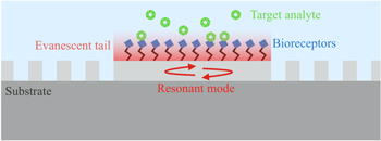
Figure 2. Illustration of the evanescent wave detection scheme for a PhC cavity. The resonant mode is confined via the photonic band gap, i.e. because the nearby holes act as reflectors. The mode is sensitive to the cover medium because of the overlap of the evanescent tail. The surface is functionalised with bioreceptors showing high affinity to a specific analyte in solution. Any binding event modulates the effective index of the optical mode, thereby causing a shift of its resonance wavelength.
Download figure:
Standard image High-resolution image2.2. Guided mode resonances
The second class of structure operates with quasi-guided or leaky modes known as GMRs [20, 21]. Similarly to strictly guided modes, GMRs confine energy in the slab, but unlike them, energy can readily couple to external radiation. This ease of interfacing provides an efficient way for coupling power into and out of the slab to facilitate the sensing function.
GMRs can be excited in wavelength-scale gratings. For a judicious choice of parameters, they exhibit a sharp peak in the reflection spectrum at normal incidence, as shown in figure 3. The grating also acts as a waveguiding layer, but, since the 'waveguide' is not homogeneous, the guided mode scatters at each interface giving rise to coherent scattering. By engineering the period, refractive indices, angle of incidence and polarisation, the phase can then be tuned in order to ensure destructive interference between the transmitted light and the power scattered upward by the leaky mode, resulting in a reflectance peak with up to 100% efficiency. As in figure 2, the quasi-guided mode is sensitive to the RI of the cover medium, providing the mechanism for sensing. By comparing the inset of figure 3 with figure 2, we note that the GMR has a larger mode overlap with the cover medium, leading to a higher sensitivity than the non-leaky guided modes, as will be discussed in section 5.
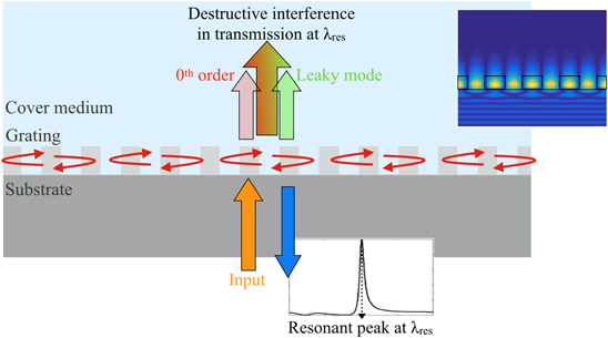
Figure 3. Diagram of a guided mode resonance (GMR) excited in a wavelength-scale grating. The grating only exhibits one diffracted order, which, for normal incidence (orange arrow), couples into the grating plane and excites the quasi-guided or leaky modes which take the form of standing waves oscillating in the plane (red arrows along the grating). They also scatter power upwards (translucent green arrow). Upon careful design of the structure, the transmitted 0th order (pink arrow) and the upward scattered leaky mode interfere destructively at a specific wavelength λres, resulting in a strong reflection peak. The inset shows the field distribution on resonance.
Download figure:
Standard image High-resolution imageFurthermore, even though the GMR is a global mode, the resonance condition depends on the RI at the specific location, so can be used for spatially resolved sensing, i.e. RI-based imaging, as will be illustrated in section 5.1.
Before we consider specific sensing geometries based on these PhC structures, let us consider the properties that make good sensors.
3. Figures of merit of a (bio)sensor
Comparing biosensors based on different technologies is not trivial because of the difficulties in defining a universal figure of merit (FOM). In fact, the performance of a biosensor depends on a number of factors. Firstly, the optical properties of the transducer need to be considered, such us the Q factor, the mode distribution, the reflection or transmission spectrum and the active sensing area. Secondly, even for the same optical characteristic, the biological protocols for surface functionalisation can affect the outcome depending on the quality of the bioreceptor layer and its binding affinity to the surface; for example, a gold surface readily binds to thiol-groups attached to a bioreceptor, while a silicon or silica surface first requires silanisation to create free amine groups on the surface to which bioreceptors can bind. Finally, the specific setup influences the accuracy of the measurement, especially in terms of adding sources of noise. Doing all of these effects justice would be well outside the scope of this paper, so we focus on the photonic aspects.
3.1. Wavelength bulk sensitivity and LOD
A key contributor to the FOM of a (bio)sensor is its sensitivity. Sensitivity is defined as the ratio between the change in sensor response, typically the wavelength change dλ, and the change in the value of the measurand, typically the RI change dn. Hence, the sensitivity represents the shift in wavelength per unit change of RI (Sλ = dλ/dn) and is quoted in nm/refractive index unit (RIU). Sλ is obtained by plotting the position of the resonance for different known values of the RI and calculating the slope of such a curve. In general, changes in refractive index due to binding events are such that the calibration curve Sλ(n) follows a linear behaviour. In fact, the evaluation is usually performed by employing water:ethanol or glucose solutions at different concentrations, which provide index variations of the order of 10−2 RIU.
The FOM is then a combination of Sλ with the smallest detectable wavelength shift, which together yield the LOD. The LOD is the smallest change in the measurand that produces a detectable change in the sensor response. The smallest measurable response RLOD is defined as [22, 23]:

where Rblank is the mean response in the absence of the measurand and σblank the associated noise (i.e. the resonance wavelength and the associated fluctuations prior to any binding event). RLOD is basically the smallest response that allows us to discriminate between the presence and the absence of the measurand. In practice, the absolute value of Rblank is not required as only the relative changes in sensor response upon binding are usually measured. In fact, the LOD is calculated by dividing 3σblank by the sensitivity, so it is expressed as the minimum change in RI that would produce a response equal to 3σblank. The assumption behind this definition is that the values of the measured sensor response (typically a resonance wavelength) are normally distributed [24, 25]. Therefore, the 3σblank rule implies a confidence of 99.7% that a change in response is actually caused by a binding event. While the sensitivity strictly depends on the physical mechanisms involved in the interaction between the radiation and the biolayer, the noise level (σblank) (and the LOD as a consequence) depends on the measurement configuration and the data analysis procedures. This means that even the same sensor system can show different values of LOD.
The measurement in resonant systems then involves determining the spectral position of the resonant peak and how much it shifts. Two main sources of noise can be identified, namely intensity and wavelength noise [24, 26]. Sources of intensity noise are typically related to photodetector noise and to fluctuations of the light source intensity, while wavelength noise comes from instability in the wavelength emitted by the source and temperature fluctuations that influence the resonator by slightly modifying its resonance condition; both effects deteriorate the signal to noise ratio (SNR) of the system.
3.2. Minimum detectable wavelength shift
The second contributor to the LOD is the smallest wavelength shift that can be detected, which is directly proportional to the Q factor; the Q factor measures the sharpness of the peak as the ratio between its centre frequency and its full width at half maximum (FWHM). Sharper peaks (higher Q) are easier to track and it has been demonstrated that in the intensity noise-limited regime, σblank depends linearly on the linewidth Δλ of the peak which means that the minimum detectable shift is inversely proportional to the Q factor [24]. However, the matter is not trivial. For very high Q factors, the peak becomes more sensitive to wavelength noise, which affects narrow peaks more significantly. In this regime, which holds for resonators with a Q ∼ 105 or higher, temperature variations become the main sources of noise and the smallest detectable shift only increases with √Q [26]. Furthermore, it becomes impractical to measure very sharp peaks because of the need for very precise spectrometers, or very fine-tuneable narrow-bandwidth sources to probe the response of the resonator. Also, high Q values typically imply that the optical mode is more strongly confined to the cavity material, meaning that the overlap with the analyte is reduced and so is the sensitivity.
3.3. Overall FOM
Having considered sensitivity and sharpness of the resonance curve, it makes sense to define the overall FOM as the product Q*Sλ [27]. Typical values for standard SPR sensors lie in the range of 104 nm/RIU (Q ≈ 10 and S ≈ 103 nm/RIU) (see table 1), which is similar to standard GMR-based sensors (Q factor and S both around 102) (see table 1). PhC cavities perform better (FOM 106–107 nm/RIU) due to extremely high Q factors (up to 105 between devices used for actual sensing), even if sensitivies are typically smaller (usually 102 nm/RIU or lower) (see table 1). However, relating these FOMs to the actual sensing capabilities in terms of the achievable LOD is not trivial because measurement noise and different functionalisation protocols significantly influence the measurement. The FOM can therefore only be considered a good indicator or starting point for the expected performance of a sensor. One can argue that for the same noise level (i.e. same value of σblank) higher FOM sensors are favoured [24]. Some examples illustrating the interplay between these different factors are presented in section 4.6.
Table 1. General overview of PhC-based biosensor.
| Structure | Analyte detected | Surface chemistry | Q factor | Bulk sensitivity (nm/RIU) | FOM (nm/RIU) | LOD | References | Notes |
|---|---|---|---|---|---|---|---|---|
| 2D PhC-in line point defect | Glycerol:water | None-only bulk sensitivity measured | ∼400 | ∼183 | 7.3 × 10⁴ | \ | [34] | |
| 2D PhC-in line point defect | BSA protein | APTES + glutaraldehyde | ∼4000 | \ | \ | 2.5 fg | [35] | |
| 2D PhC-side-coupled point defects | Human IgG protein | APDMES + glutaraldehyde + anti IgG | 400 | 64.5 | 2.6 × 10⁵ | 10 μg ml−1 1.5 fg | [36] | |
| 2D PhC-side-coupled point defects | HPV virus-like particles | APDMES + glutaraldehyde + HPV16 L1 antibodies | ∼1500 | 64.5a | 9.7 × 10⁵ | 1.5 nM | [37] | |
| L21 slow light engineered cavity | Avidin | 3-APTES + glutaraldehyde + inkjet printed antibodies | 7300 | 66 | 4.8 × 10⁵ | 67 pg ml−1 | [44] | |
| L55 slow light engineered cavity | Avidin | 3-APTES + glutaraldehyde + inkjet printed antibodies | 14 000 | 74 | ∼106 | 3.35 pg ml−1 | [44] | |
| L3 cavity | BSA | None-only physisorption | 5100 | 101 | 5.1 × 10⁵ | 10 ng ml−1 | [45] | |
| Slotted W1 PhC waveguide | Glucose solutions | None-only bulk sensitivity measured | 4000 | 1538 | 6.1 × 10⁶ | 7 × 10⁻⁶ RIU | [50] | |
| Slotted W1 PhC waveguide | Avidin | APTES + biotin/DMF/PBS | ∼6000 | 500 | 3 × 10⁶ | 1 μg ml−1 (0.1 fg) | [51] | Sensitivity is theoretical |
| Slotted nanobeam cavity | Glucose solutions | None-only bulk sensitivity measured | 500 | 700 | 3.5 × 10⁵ | \ | [48] | Luminescence from QDs |
| Nanobeam cavity | GFP | None-optical trapping | 2000 | \ | \ | 260 ng ml−1 | [59] | Optical trapping of NPs clusters |
| Nanobeam cavity | Wilson disease protein | None-optical trapping | 5000 | \ | \ | Single protein | [60] | |
| H0, H1, L3 | E. coli and B. | None-optical trapping | 2300 | \ | \ | Single | [62] | |
| cavities | subtilis | bacteria | ||||||
| Nanobeam cavity | S. epidermidis, E. coli and B. subtilis | None-optical trapping | 4000 | \ | \ | Single bacteria | [63] | |
| Nanobeam cavity | CEA antigen | APTES + glutaraldehyde/sodium cyanoborohydrite + anti-CEA | 9000 | 70 | 6.3 × 10⁵ | 0.1 pg ml−1 | [67] | |
| SPR (Biacore) | CEA antigen | MUDA + EDC-NHS + anti-CEA | ∼2 × 10 | ∼103 | ∼ 104 | 3 ng ml−1 | [68] | |
| SPR imaging | ssDNA | ∼10 | ∼103 | ∼104 | 50 nM | [69] | ||
| W1 PhC waveguide | ssDNA | 3-isocyanatopropyl triethoxylane vapour + streptavidin + biotinylated ssDNA | \ | \ | \ | 20 nM | [70] | |
| GMR on 2D grating | BSA Streptavidin | APTES + s-SDTB + NHS-PEG-biotin | ∼150 | 88 | 1.3 × 10⁴ | 1 ng ml−1 | [94] | |
| GMR on 2D grating | Avidin | Poly-phe-lysine + NHS-LC-biotin | ∼200 | 88a | 1.7 × 10⁴ | 1 μg ml−1b | [95] | |
| GMR on 2D array of holes | Different solutions | None-only bulk sensitivity measured | ∼85 | 510 | 4.3 × 10⁴ | \ | [99] | |
| GMR on 1D grating | Protein A | Human, sheep, chicken IgG + protein A | ∼240 | ∼300 | 7.2 × 10⁴ | 0.5 mg ml−1b | [100] | Porous glass substrate enhancement |
| GMR on 1D grating | Biotin | Amine film + glutaraldehyde + streptavidin | ∼290 | ∼300a | 8.7 × 10⁴ | 1 mg ml−1b | [101] | Porous layer enhancement |
| GMR on 1D grating | TNF-α Calreticulin | APTES + DSS + antibodies | Not reported | Not reported | \ | 156 ng ml−1 390 ng ml−1 | [102] | Dual polarisation |
| GMR on 1D grating | Biotin Estradiol | Amine film + glutaraldehyde + streptavidin/estrogen receptor α (ER) | 2.8 × 10⁷ | 212 | 5.9 × 10⁹ | 260 ng ml−1b 136 ng ml−1b | [104] | GMR as feedback element of an ECL |
| GMR on 1D grating | Sucrose solutions | None-only bulk sensitivity measured | \ | 6 × 10³π rad/RIU | \ | 3 × 10⁻⁷ RIU | [110] | Interferometric |
| Bi-modal waveguide | HCl solutions | None-only bulk sensitivity measured | \ | 6 × 10²π rad/RIU | \ | 2.5 × 10⁻⁷ RIU | [114] | Interferometric |
| Bi-modal waveguide | E. coli | APTES + PDITC + anti E. coli antibodies | \ | 6 × 10²π rad/RIUa | \ | 4 cfu ml−1 | [116] | Interferometric-in ascitic fluid |
| Chirped | IgG protein | APTES + EDC/NHS + anti IgG | \ | 137 | \ | 38 ng ml−1 | [119] | |
| GMR on 1D grating | CD40 antibody EGF antibody Streptavidin | APTES + PDC + various ligands | \ | \ | \ | 13.5 μg ml−1b 13.5 μg ml−1b 30 μg ml−1b | [123] | Intensity and in parallel detection |
| GMR on 2D grating | ||||||||
| GMR on 1D grating | TNF-α | NaOH + O2 plasma + GPTS + antibody (Mab1) | ∼80 | \ | \ | 1.6 pg ml−1 | [150] | Cy-5 fluorescence enhancement |
| GMR on 1D grating | DNA (microarray) | O2 plasma + 3-glycidoxypropyltrimethoxysilane + printed oligonucleotides | ∼50 | \ | \ | \ | [151] | Cy-5 fluorescence enhancement |
aAssumed to be the same as previous work(s) from the same research group because of the structure being the same. bThe experiment has been conducted only with the reported concentration of analyte(s) and/or the signal to noise ratio is still over the 3σ threshold, therefore the actual LOD could be potentially smaller than the reported value.
3.4. Surface sensitivity
The above figures refer to what is known as the bulk sensitivity, which describes the sensor response to changes in the entire cover medium. The bulk sensitivity is certainly useful for calibrating the performance of the sensor against media of known refractive index, such as glucose solution or ethanol:water mixtures. It is also meaningful when considering the detection of large targets, such as cells and bacteria, which represent a bulk RI change due to their size being typically larger than the exponential tail of the optical mode. In most cases, however, the sensor is designed to detect molecular binding events, which occur very close to the surface. Hence, we need to define the surface sensitivity as the wavelength shift upon surface molecular binding.
A general relation between the bulk and the surface sensitivity has been derived in Zhu et al [28] for ring resonators. A similar procedure for converting bulk sensitivity to surface sensitivity can be applied to all resonant-based RI sensors [24, 28]. Several parameters contribute to determining the surface sensitivity, such as the polarizability and the surface density of the biomolecule layer. Nevertheless, as demonstrated in [27, 29] for GMR-based devices, it is difficult to produce a general rule and results strongly depend on the nature of the mode. In particular, the position of the modal axis has to be taken into account (that is the centreline through the resonant mode along the structure) as well as the effective index (neff) and the penetration depth into the medium.
The effective index neff can be considered as an average refractive index weighted by the field distribution of the mode and, together with the index of the cover medium (nc), it determines the decay length of the evanescent tail. For instance, for a waveguide mode the decay constant γ can be expressed as:

The larger γ, the shorter the decay length, which means that the overlap between the evanescent wave and the biolayer is increased. This concept leads to the definition of a detection zone as the fractional field intensity integrated over the spatial regions occupied by the biomolecules [29]. The overlap should be maximised as those parts of the field that do not overlap with the biolayer do not contribute to the sensitivity.
4. PhC cavity-based devices
PhC cavities offer strong confinement and high Q factors. Sensing volumes are very small, which is particularly convenient for sensing in small spaces, such as inside single cells or in their neighbouring regions. Their footprint is also very small, making them suitable for multiplexing and arraying.
4.1. Single cell techniques
Probing individual cells is advantageous for a number of reasons [30, 31], mainly because probing a large number of individual cells and studying their differences in metabolism, morphology or response to drugs provides more information due to their natural heterogeneity, even within the same tissue or community. Traditional techniques, such as ELISA, only provide average information on ensembles, thereby missing underlying distributions of cell properties. Conversely, statistically rich single cell data provide insight into cell heterogeneity by identifying, for example, subpopulations that have adopted specific strategies for survival, infection or cancer development.
Moreover, such techniques allow sensing in vitro, so the cell is probed in a viable status with minimal interferences with its natural physiology; in vitro techniques also afford time-dependence, so the evolution of cells can be tracked. On the other hand, traditional techniques require fluorescent labelling of intracellular compounds, which imply cell lysis and only provide a single snapshot. In fact, the ability to probe individual cells and to track them over time also applies to GMR-based devices, as we will discuss later, in particular in section 5.1.
A very exploratory and compelling example for the ability of PhC cavities to probe inside living cells is presented in [32]. The authors connected a PhC nanobeam cavity to a multimode fibre (shown in figure 4(a)) which collects the luminescence signal from quantum dots (QDs) embedded in the cavity. The cavity is then inserted into a PC3 cell, i.e. a common human prostate cancer cell line (figure 4(b)), and the luminescence is stimulated by pumping the QDs with a laser. Surprisingly, a high fraction of the cells exposed to this treatment remained viable and continued their normal functions, including division. Totally internalised probes (i.e. cleaved from the fibre) are even passed onto daughter cells, which continue to grow. No actual intracellular sensing was performed but this configuration paves the way for future developments in which the probe can be functionalised in order to bind specific intracellular compounds.

Figure 4. (a) Nanobeam cavity mounted on the tip of an optical fibre. The inset shows a close-up of the very tip. (b) The probe is gently inserted inside a single cell with the aid of micro positioners. Reprinted with permission from [32]. Copyright (2013) American Chemical Society. (c) Array of hollow PhC cavities side-coupled to the same W1 guide and placed on PDMS. The cavities have slightly different resonant wavelengths so can be individually addressed by wavelength division multiplexing (d). Reproduced from [33]. CC BY 4.0.
Download figure:
Standard image High-resolution image4.2. Multiplexing
A similar experimental approach was demonstrated by Scullion et al [33], who transferred an array of PhC cavities onto a PDMS substrate to enable in situ measurements. The cavities were excited via a tapered optical fibre (see figures 4(c) and (d)). The authors demonstrate the multiplexing capability of this arrangement by slightly tuning the resonant wavelength of each cavity, such that the location can be mapped onto a particular spectral line, akin to the wavelength division multiplexing method. The cavities were all side-coupled to the same bus waveguide and excited at different wavelengths, which allowed mapping RI changes both in time and space. The authors chose a hollow cavity, which is advantageous because a large fraction of the cavity mode overlaps with the medium, thereby increasing the sensitivity. The same idea is exploited in the slotted cavities that will be presented in section 4.4.
Another type of defect that allows multiplexing is a point defect, in which the diameter of a single hole is instead reduced. Chow et al [34] first demonstrated such a structure for an in line propagation configuration. They obtained a sensitivity of 183 nm/RIU and measured the refractive index of a glycerol:water mixture. Lee et al [35] later adopted a similar configuration showing that 2.5 fg of BSA protein produced a detectable signal as a shift of the transmission peak. Subsequently, the same point defect was employed in a side-coupled scheme [36]. A W1 PhC waveguide was created in a typical hexagonal lattice and the defect is introduced by modifying the radius of a single hole next the W1 waveguide. In this case, a dip in the transmission spectrum with Q ∼ 103 is observed and tracked, like in the side-coupled Ln cavities (see figure 1(a)). This configuration is suitable for multiplexing, as shown in [37]. Up to three cavities have been fabricated in series in order to produce multiple dips to be tracked and potentially to be functionalised with different bioreceptors. Virus-like nanoparticles with a diameter of 55 nm have been detected down to a concentration of 1.5 nM in serum.
4.3. Slow light engineered cavities
Another attractive feature that can be exploited on the PhC platform is the phenomenon of slow light. The aim of slow light is to enhance the light–matter interaction [38, 39]. By combining slow light engineering with side-coupled cavities, such as the Ln series, typical values of Q are in the high 103 and sensitivities around 100 nm/RIU [40, 41]. In addition, Ln cavities can be made longer, such as L13, L21, even up to L55 in order to provide even higher Q factors [42]. Increasing the Q factor is an obvious consequence of lengthening the cavity, but increasing the length of the cavity also implies that the supported modes move closer to the band edge of the W1 waveguide that supports them. Correspondingly, the group index increases, and the slow light effect is enhanced. Lai et al show that this effect increases the sensitivity, which is quite remarkable; they measured a doubling in sensitivity for a L13 cavity compared to a regular L3 together with a Q factor increase by almost 1 order of magnitude (from 5 × 10³ to 3 × 10⁴). To evidence this improvement, the reported LODs for slow light engineered L13 and L55 cavities are 670 pg ml−1 for the cancer marker ZEB1 (Q factor of 13 000) [43] and 3 pg ml−1 for avidin binding to biotin (Q factor of 14 000) [44]. Conversely, the standard L3 cavity investigated in [45] showed a relatively lower LOD of only 2.4 × 10⁻³ RIU and a lower LOD of 10 ng ml−1 for BSA.
4.4. Slotted cavities
An interesting variant of the PhC cavity configuration is the slotted cavity [7, 46]. Slotted cavities combine the concept of PhC confinement with the slot waveguide [47] by adding an air slot at the centre of the cavity. Slots can be applied to a variety of structures, such as 1D nanobeam cavities [48] or 2D cavities [49]; their main advantage is a strong spatial confinement of the mode within the air slot and the resulting larger overlap of the mode with the sensing medium, which increases sensitivity. Indeed, slotted devices show the best performance in terms of sensitivity and LOD within the class of PhC biosensors. While standard PhCs exhibit sensitivities in the range 50–100 nm/RIU, slotted configurations reach values of 500 nm/RIU, with the highest reported value being 1500 nm/RIU with a Q factor of 5 × 10⁵ and an LOD of 7 × 10⁻⁶ RIU [50] (see also table 1). In order to achieve these values, di Falco et al added the slot to a W1 waveguide and used the heterostructure geometry (figure 1(c)). In another work from the same group [51], the authors employed the same structure for the detection of avidin, with a LOD of 1 μg ml−1 and estimated bound mass of only 0.1 fg. Wang et al [48] covered their slotted nanobeam cavity with a single layer of QDs and monitored their luminescence, which was an interesting modification. They achieved a sensitivity of 700 nm/RIU with a Q factor of 500. More recent theoretical work points at further improvements. For example, Sun et al [52] have simulated rectangular air holes and predict a sensitivity of 835 nm/RIU with a Q factor of 5 × 10⁵. Zhou et al [53] have used two coupled nanobeam cavities and predict 435 nm/RIU with a Q of 107. These results suggest that further experimental improvements may be following shortly.
4.5. Optical trapping
As an aside, slow light engineering and PhC cavities can also be beneficial for improving the performance of optical traps. Scullion et al [54] have shown that slow light engineering leads to an enhancement in the guiding of sub-micron particles along a slow light engineered W1 waveguide as well as of the trapping stiffness, which allows for longer and stable trapping. Indeed, optical trapping benefits from PhCs, mainly because of the strong confinement that is achieved in the nanophotonic environment as well as the small values of power required if compared to traditional free-space laser beam trapping. An exhaustive review can be found in [55]. Briefly, the main FOM for optical trapping is the Q/V ratio, where Q is the Q factor of the resonator and V the modal volume. PhC structures can provide remarkably high Q/V values. For example, in the L3 cavity, the modal volume is typically of order of (λ/n)3. By engineering the hole positions and radii surrounding the cavity, the modal volume can be reduced by almost one order of magnitude [56, 57]. Similarly, slotted versions of the L3 and the nanobeam cavity can achieve values as low as 10−2(λ/n)3 [58]. Another contender in terms of Q/V are plasmonic structures because of their extreme confining capability, which can push the modal volume down to 10−3(λ/n)3. However, Q factors are usually much lower, i.e. of order of a few tens. The other issue is heating, which is often associated with plasmonic structures and which may cause increased Brownian motion that reduces the trapping stability.
Cavity-based optical trapping also offers significant advantages for biosensing by overcoming the need for the analyte of interest to bind or physically adsorb on the sensing surface. This process requires a surface functionalisation step and the use of bioreceptors, which make the device difficult to reuse. Conversely, optical trapping is often reversible and breaks the diffusion limit to a certain degree, thanks to the optical forces dragging particles to the cavity [59]. However, these benefits come at the cost of a loss of selectivity.
Selectivity can be retrieved by employing, for example, functionalised nanoparticles which are then optically trapped by the cavity. In [59], polystyrene particles are coated with anti-GFP (green fluorescent protein, 26 kDa) antibodies. Binding of target protein causes the particles to aggregate into clusters which are then optically trapped by a nanobeam cavity with a Q ∼ 2000. The method is proven to be quantitative, as different concentrations of GFP result in different levels of aggregation of the nanoparticles, causing in turn a different shift in resonance wavelength upon trapping. The lowest concentration detected was 10 nM (260 ng ml−1). Another example of protein trapping is reported in [60], where a nanobeam cavity in silicon nitride with a Q ∼ 5000 is employed to trap and release single Wilson disease proteins as well as 22 nm polymeric particles.
Specific antibodies-proteins and antibodies-viruses interactions at the single molecule level have also been studied with a nanobeam cavity by Kang et al [61]. The authors exploited the fluctuations of the power transmitted through the cavity to detect protein-antibodies binding events. Single influenza viruses A were imaged through the near-field light scattering techniques, which consist in detecting the near-field light scattered by the trapped viruses, allowing to image with a standard microscope and without the need for any fluorescent tag.
Optical trapping based on PhC cavities is particularly advantageous when localisation of single cells is required. Van Leest and Caro [62] reported trapping of single bacteria (Bacillus subtilis and E. coli) with a PhC for the first time by employing H0, H1 and L3 cavities. A 1D nanobeam cavity was later employed for localising single bacteria and tracking their movement patterns. Fluctuations of the power transmitted through the cavity have been shown to depend on bacterial morphology, such as size, shape and presence of flagella, allowing in turn for a precise classification of different types of bacteria [63]. Localisation is also required for performing Raman spectroscopy or surface enhanced Raman spectroscopy on single entities. This has been shown on single Ag nanoparticles by Lin et al [64].
An interesting configuration has been recently proposed by Jing et al [65] to overcome the difficulties of light coupling and confinement in integrated platforms. The authors proposed a 2D PhC slab patterned with a square array of holes and illuminated with a loosely focused beam from the top. The periodicity of the pattern modulates the reflected light and generates a focused volume at a certain distance from the surface, which acts as the trapping spot. The device was then employed for the optical trapping of eukaryotic yeast cells and E. coli bacteria. Cells remained viable for more than 30 min of trapping.
4.6. Comparison with SPR-based devices
We now use a PhC nanobeam cavity as an example for comparing the PhC platform with the well-established surface plasmon resonance (SPR) platform. This comparison serves to illustrate how the interplay between the Q factor and the sensitivity contributes to the sensing performance.
We use the detection of the carcinoembryonic antigen (CEA) as an example, which is a well-known colorectal cancer marker of mass 180 kDa [66]. Liang et al have demonstrated an LOD of 0.1 pg ml−1 for CEA by using a nanobeam cavity with a bulk sensitivity of 70 nm/RIU and a Q factor of order of 104 [67]. For the same biomarker, SPR-based devices are able to reach 3 ng ml−1 e.g. with the Biacore system [68]. Although the two sensors feature comparable FOMs (considering the typical values of Q ∼ 10 and Sλ ∼ 103 nm/RIU for a plasmon mode), Liang et al reached 4 orders of magnitude lower LOD. This improvement is likely due lower levels of wavelength and temperature noise as well as a better functionalisation protocol.
To highlight the variability of such comparisons, another example is DNA detection, whereby complementary DNA strands are immobilised on the surface in order to bind to the complementary strain in the analyte. Traditional SPR platforms exhibit an LOD in the order of tens of nanomolar for such a system. For example, in [69] single strand DNA is detected with SPR imaging and an LOD is 50 nM is achieved. A W1 PhC waveguide has been shown a similar limit of 19.8 nM [70]. In this particular work, the authors track the position of the cut-off wavelength of a W1 PhC waveguide. Even though the geometries are very different, the detection limit is remarkably similar.
These examples clearly illustrate the interplay between FOM, functionalisation of the surface and noise in determining the LOD. Even though FOMs are comparable, in the first one PhCs perform better, whereas in the second one performances are similar. Differences in the LOD can thus be ascribed to different functionalisation protocols and handling of the sources of noise.
4.6.1. Mechanisms of sensing and extraordinary SPR sensitivity
The strength of SPR techniques is their much higher sensitivity compared to dielectric resonances (typically above 1000 nm/RIU, up to over 7000 nm/RIU in some cases [71]), yet the FOM tends to be lower because of the very low Q factor typical of plasmon resonances, which is of the order of only 10–20. Indeed, SPR sensing relies on the high sensitivity of the plasmon mode, which arises from the peculiar dependence of the resonance condition on the RI. Let us compare.
Both PhC and SPR are based on guided modes and are governed by guided mode theory, which stipulates that the exponential tail of the mode into a dielectric cladding is given by equation (2). According to this equation, the extent of the evanescent tail is only given by the difference between the effective index of the guided mode and the index of the cladding. The effective index of a plasmon mode is typically 1.5–1.7 and that of a dielectric mode is between 1.5 and 2.5, with the cladding typically being water. This results in decay lengths between 100 and 200 nm [18, 72, 73].
PhCs typically rely on single mode resonances excited in dielectric cavities whose effective index is modulated by binding events happening within the evanescent tail. Perturbation theory predicts an upper bound for the wavelength sensitivity, which, for the case of 100% overlap of the mode with the medium, suggests that dλres/dn ≈λres/n, which typically assumes a value of a several hundreds as the maximum possible sensitivity [74]. SPR sensitivities clearly exceed this limit. The reason for their high sensitivity lies in the very nature of the transduction method, which relies on wave vector matching between the incident radiation ki(ω) and the travelling plasmon wave at the metal-dielectric interface kpl(ω, nc), where nc is the refractive index of the cover medium. The dispersion of ki(ω) is represented by a straight line, whereas kpl(ω, nc) is the typical plasmon dispersion curve. The resonance wavelength is determined by the crossing of the two curves, i.e. ki(ω) = kpl(ω, nc) must be satisfied. A prism or a diffraction grating is usually employed to impart the necessary momentum to ki for the two curves to intersect. The slight curvature of the plasmon curve then makes the intersection highly dependent on refractive index changes, which provides a natural amplification mechanism, so when nc changes, the plasmon curve only need to tilt by a small amount to produce a large shift in wavelength.
A more detailed description of this effect can be found in [74, 75] for different configurations and interrogation modalities. Overall, the significant difference in sensitivity achieved between the two systems is based not on differences in the evanescent tails of the respective modes, but on k-vector matching and the excitation of a propagating wave in the SPR case versus exciting a standing wave in the resonator case.
Nevertheless, despite the higher sensitivity of SPR, their low Q factor prevents achieving a very low LOD. In other words, the FOM = QSλ, even though being a guideline only, highlights why high Q factor cavity systems generally perform better than SPR systems.
4.6.2. General remarks on PhC cavities compared to SPR
Despite this apparent inferiority, SPR devices are widely used commercially, whereas PhC cavity-based sensors are not. The reason is the relative ease of use and simplicity of the SPR system, which brought SPR to the market as early as the 1980s (GE Healthcare, Chicago, USA). In contrast, PhCs have stringent fabrication tolerances and typically require electron beam lithography for their fabrication, which makes them more suitable for laboratory use and for fundamental studies. Where PhC devices may gain an advantage is in the area of multiplexing, because of their much smaller footprint, so one can imagine systems that, together with modern spotting techniques, can interrogate tens or hundreds of different binding events in parallel. In fact, the idea of multiplexing has already been realised with microring resonators, which, similar to PhC cavities, operate on a small footprint, as we will discuss next.
In terms of practicalities, both classes have various disadvantages which limit their use to laboratory science rather than clinical practice. They usually require the use of a laser. SPRs need an external prism or grating and a precise control over the incident angle to excite the plasmon wave. PhCs require grating couplers or end-fire setups to couple light and bulky spectrometers or diffractive elements to resolve the narrow resonance. They are both still at the 'chip-in-a-lab' stage rather than the desired 'lab-on-a-chip' configuration, which is essential to enable a true on-field or clinical application outside of research laboratories.
The difference in performance between SPR and GMR-based sensors will be discussed in section 5. GMR performs at a similar LOD level as SPR, but the intrinsic simplicity of coupling and collection light makes them very attractive for future commercialisation.
4.7. Comparison with microring resonator devices
Microring resonators are another attractive platform for biosensing and they currently represent the most exploited alternative to the widespread SPR platform. In-depth reviews can be found elsewhere [76–78]. In the context of this review, it is instructive to briefly compare them with PhC-based devices to highlight strengths and weaknesses.
The sensing principle of a microring is also based on the evanescent tail mechanism. The optical mode is a whispering gallery mode (WGM) supported by a ring-shaped waveguide side-coupled to an adjacent straight waveguide (access waveguide). Given the length of the ring, a WMG is excited when an integer multiple of its wavelength fits into the loop. This results in equally spaced dips in the transmission spectrum of the access waveguide, because of the destructive interference between the access waveguide mode and the light coupled back from the ring. As in the case of the PhC cavity, the position of the resonance is tracked upon binding.
In terms of biosensing, the main advantage of microrings over SPR is their reduced footprint, which enables them to perform multiplexed measurements. This feature has made them the main competitors to SPR technologies, in particular for commercialisation. For example, Genalyte (Genalyte, San Diego, CA, USA) has developed MaverickTM, a platform based on ring resonators to detect up to 32 analytes in parallel in as little as ten of minutes [79, 80]. Microrings also perform better in terms of the Q*Sλ FOM. Sensitivies are usually lower than SPR, in the order of tens of nm/RIU, however Q factors are comparable or even higher than typical PhC cavities. Depending on wavelength, material and geometrical parameters, values lie in the range 104–108 [76, 77, 81–83]. Compared to PhC cavities, they are more tolerant to fabrication imperfections, although the precision of the gap between the access waveguide and the microring critically determines the achievable Q factor.
The reason for their low sensitivity is the strong confinement of the resonant mode in the guiding medium, which means that the overlap with the sensing medium is small. Different strategies have been employed to enhance this sensitivity, with slotted configurations being the most promising approach. Slotted configurations offer the same advantages as already mentioned for PhC structures, i.e. increased overlap with the sensing medium, and correspondingly higher sensitivities, i.e. up to 300 nm/RIU [25, 84]. Even larger values of the order of 2000 nm/RIU have been demonstrated by employing a Vernier effect configuration with two cascaded rings [85].
Another interesting possibility for enhancing sensitivity is the combination between the concepts of PhCs and ring resonators. This configuration has been recently studied by Lee et al [86] and proposed for sensing by Lo et al [87]. The microring structure has been periodically patterned with circular holes along the ring circumference. A sensitivity of ∼250 nm/RIU has been measured, which featured a two-fold increase compared to control microrings with no holes. The reason is that a significant fraction the optical mode on resonance is located inside the air holes, thereby increasing overlap with the cover medium. In addition, slow-light effects are observed. However, the Q factor is reduced to ∼1200, which does not lead to an overall increase of the FOM. Specific DNA and protein binding has been performed. The lowest measured concentration of streptavidin was 20 nM, but the corresponding wavelength shift of 0.18 nm is likely well above the minimum detectable shift.
Integration of standard microring resonators with electrochemical measurements has also allowed to measure the conformation and thicknesses of molecular layers, which is not a typical ability of most biosensors operating only in the optical domain [83].
The major disadvantage of microring resonators in the context of POC devices is the common downside to all integrated sensors, namely the need for accurate light coupling and detection imposed by the use of single mode waveguides. Such waveguides are necessarily only micron-sized, which requires the use of angle and wavelength sensitive grating couplers or end-fire setups that need active alignment, although we note that progress has been made very recently by way of demonstrating an LED-based flood-exposure system compatible with grating couplers [88].
5. GMR sensors
A GMR is a leaky or quasi-guided mode supported by a periodically patterned slab [20, 21], aperiodically ordered supercells [89–91] or compound structures obtained by superposition of two or more single-period structures [92, 93]. These modes readily couple to external radiation and they can be easily excited. Typically, collimated light is used at normal incidence and the reflected or transmitted spectrum is collected. Geometrical parameters and materials can be tuned in order to obtain a resonance peak of Q ∼ 100–200. The phase-matching condition determining the peak wavelength is dependent on the refractive index of the cover material, providing the mechanism for sensing. Here, we focus on some of the applications that demonstrate the degrees of freedom offered by the GMR approach, how their performance can be enhanced and how they compare to cavity-based and SPR sensors.
We will devote particular attention to one-dimensional wavelength-scale gratings that support a GMR based on the pioneering work of Magnusson [20] and Cunningham [94, 95], who highlighted the possibility of using GMRs for sensing applications and then showed the possibility of detecting streptavidin down to ng ml−1 levels. Cunningham et al also demonstrated the detection of DNA-protein binding, sequence-dependent binding and highlighted the inhibition mechanisms of these interactions [96]. The same group has also shown the possibility of employing the GMR structures with an inverse assay platform by using functionalised iron oxide nanoparticles for the detection of soluble transferrin reception [97].
A typical measurement scheme is illustrated in figure 5(a) along with 3D sketch of the grating and a SEM picture in figures 5(b) and (c) (from [98]). One of the main limitations of GMR-based sensors is their modest sensitivity (usually of the order of 100 nm/RIU) and Q factor (of the order of 100), limiting the LOD to the range of 10−5 RIU (refer to typical examples reported in table 1). Different strategies have been proposed to overcome these limitations.
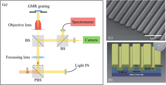
Figure 5. (a) Schematic of a typical measurement setup used to measure reflection of a GMR grating. PBS stands for polarising beam splitter which ensures polarisation selection. BS is a normal beam splitter. The lens focuses onto the back focal plane of the objective lens in order to collimate light incident on the grating surface. (b), (c) A typical geometry and SEM picture of the gratings used by the group of Cunningham. Reproduced from [98] with permission of The Royal Society of Chemistry. A UV-curable polymer is spun onto a glass cover slip (visible in the inset) imprinted and UV cured. The 60 nm TiO2 layer is sputtered and provides the high-index layer for exciting the GMR.
Download figure:
Standard image High-resolution image5.1. Suspended symmetric membranes
El Beheiry et al [27] simulated a variety of silicon nitride slabs suspended in free-space and patterned with a square array of holes, assuming that the analyte completely encompasses the slab. Their main finding was that the suspended geometry, due to its inherent symmetry, can exhibit Q values as high as 1.6 × 10⁵, sensitivities of almost 800 nm/RIU, and an impressive LOD of 10−7 RIU. The reason for the high sensitivity is that the bottom half-plane is also available for sensing, thereby increasing the effective sensing area. In fact, this approach had already been tested experimentally by measuring a very similar configuration in [99]. Indeed, for a judicious choice of hole radius and period, a bulk sensitivity of 510 nm/RIU had been measured, even though the Q factor was only about 100. The drawback of the suspended design is the added fabrication step and the increased fragility, which may also make the structure more susceptible to noise. Nevertheless, membranes of a relatively large area of (200 × 200) μm2) have been observed to withstand several hours of operation under flow pressure.
Another solution pointing in a similar direction consists of using a low refractive index substrate, which helps to push centre of the mode up towards the cover medium. This method was demonstrated by fabricating the grating out of a low-index porous glass with an index of 1.17 and subsequently covering it with 165 nm of high-index TiO2 to provide the necessary high-index for confining the GMR; the sensitivity increased four-fold as a result for the detection of the protein A binding to IgG antibodies [100]. The performance can also be enhanced by adding a thin layer of porous TiO2 to increase the number of binding sites available for molecular binding. This approach also led to a maximum ∼4× enhancement of the sensitivity compared to a standard design for the detection of an amine polymer film that conforms to the porous surface area in a single monolayer as well as the binding of glutaraldehyde to the amine film. The properties of the resonance were not affected significantly by the modified porous surface of the grating [101].
5.2. Sensing with different polarisation
An attractive feature of the grating is that a GMR is supported for both TE and TM polarisation (i.e. electric field parallel or perpendicular to the grating vector [21]. The two modes show different modal distributions and Q factors. In particular, the TM mode is more strongly confined and it has a smaller decay length, making it suitable for proteins and the detection of small biomolecules. The TE mode, on the other hand, extends further into the analyte and is therefore more suitable for the detection of larger objects such as cells [27].
This polarisation duality has been exploited by Magnusson [102] for detecting the tumour necrosis factor alpha (TNFα) with an LOD of 156 ng ml−1 and cancer biomarkers such as calreticulin, an early indicator of ovarian carcinoma. For the latter, the lowest measured concentration was 390 ng ml−1, but with a high SNR, meaning that even lower concentrations could have been detected. In this experiment, both TE and TM resonance peaks were tracked. The two sets of data allowed to distinguish any background index or density fluctuations from the binding events, providing a self-referencing mechanism. Additionally, two measured uncorrelated variables enable to determine two unknowns. By back fitting collected data with simulation results, both the thickness and the refractive index of the adsorbed layer can be estimated from a single experiment. This approach is very powerful as it allows to characterise layers of surface-bound molecules and to monitor changes in molecular conformation, as also recently demonstrated by Juan-Colás et al with ring resonators [83]. Nevertheless, the polarisation duality has not been extensively exploited for GMR-based devices. Furthermore, if combined with electrochemical measurements, this approach also enables direct and precise measurement of molecular density on a surface, which is not possible with SPR-based sensors, as they only support TM-polarised radiation [103].
5.3. GMR grating as feedback element
GMRs have the intrinsic property of reflecting 100% of the radiation on resonance. This feature has been exploited by using a GMR grating as the reflector of an external cavity laser (ECL) [104]. The grating then acts both as the transducer and as the wavelength selective element.
In other words, the grating is used to feed the back-reflected GMR mode into an external semiconductor optical amplifier which provides gain and sharpens the peak, as illustrated in the scheme in figure 6(a). Binding of biomolecules causes the effective cavity length to change and so does the lasing wavelength. The GMR grating itself shows a modest Q in the high 102, but its interaction with the amplifier increases this to massive Q of 107, while the sensitivity is unchanged (212 nm/RIU). This dramatically increases the FOM (Q*Sλ) by a factor 104 resulting in a LOD of 10−7 RIU, which is then limited by other system noise. An upgrade is provided by mounting two gratings on the opposite sides of a flow chamber frame [105]. In this fashion, both gratings are exposed simultaneously to the same analyte which provides a self-referencing capability by only functionalising one of the two. Since both gratings serve as wavelength selective elements for the ECL, the laser operates at two distinct wavelengths [106].
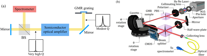
Figure 6. (a) Schematic of the ECL configuration demonstrated in [104]. The cavity is defined by the GMR on one side and the mirror on the far left. Binding events on the grating change the effective length of the cavity and cause a shift in the lasing wavelength. The gain window of the amplifier includes the GMR resonance and significantly sharpens the peak (b) schematic of the phase detection setup demonstrated in [110]. Reproduced from [110]. CC BY 4.0. The He–Ne laser beam is split to form a Mach–Zehnder interferometer which picks up the phase change of the GMR on resonance.
Download figure:
Standard image High-resolution image5.4. Phase shift detection in GMR and comparison with integrated devices and SPR
An alternative possibility for boosting sensitivity and improving performance is phase detection. The main idea is to exploit the large phase jump that occurs on resonance. The original idea dates back to 2004 [107]. First experiments showed an LOD of order 10−7 RIU. However, complex equipment and elaborate phase reconstruction algorithms were employed [108, 109]. More recently, Sahoo et al have combined GMR detection with a relatively simple Mach–Zehnder interferometer illustrated in figure 6(b) [110]. Any change in refractive index on the sensor will modify the accumulated phase and consequently shift the fringe pattern. The LOD was determined to be 3.4 × 10⁻⁷ RIU. This represents a 2–3 orders of magnitude improvement over standard GMR sensors and is a typical value for interferometric sensors, as phase detection is more sensitive than tracking wavelength.
As briefly mentioned above, interferometric sensors show the highest sensitivities and the lowest limits of detection ever reported [111]. In particular, integrated Mach–Zehnder interferometers have shown to reach LODs of 10−8 RIU [112] or even an impressive 9 × 10⁻⁹ RIU in the Young configuration [113]. An important drawback of these designs is the addition of an interferometric arm for splitting the beam. An elegant solution has recently been introduced by employing a bi-modal waveguide [114, 115]. Such a waveguide features two sections: a single mode waveguide at the beginning and a dual-mode waveguide in a second, thicker section. The two modes have a different penetration depth into the cladding medium, so they will accumulate a different phase shift upon binding and will generate an interference pattern at the exit of the waveguide. An LOD of 2.5 × 10⁻⁷ RIU is achieved with this configuration, which has led to the impressive ability of detecting 4 bacteria per ml in clinical ascitic fluid [114, 116].
Similar schemes have also been developed in the context of SPR sensing, with similar outcomes. LODs of order 10−7 RIU and even 4 × 10⁻⁸ RIU have been reported [117, 118]. The beam was either split in a Mach–Zehnder configuration or the interference between TE and TM was exploited in a 'common path' configuration. This configuration is possible because TE radiation does not excite an SPR, so it is specularly reflected, while the TM mode accumulates a phase change when exciting the plasmon resonance.
5.5. Chirped GMR
All of the resonant methods mentioned so far require wavelength tracking. Hence, the ability of discerning very small wavelength shifts is crucial, especially for the high Q methods. Resolving very small wavelength shifts requires the use of sensitive, often bulky and expensive spectrometers and adds complexity to the measurement setup. An original solution has recently been introduced by our group who used chirping of the geometrical parameters of the grating which supports the GMR mode [119] (see figure 7). In particular, the filling fraction (i.e. the width of the grooves) is tapered spatially, which makes the resonance wavelength a function of position along the grating. In this configuration, when a monochromatic source illuminates the structure, only a narrow transverse region resonates, which results in a high reflectivity strip lighting up (figure 7(d)). Any change in refractive index will cause the line to shift spatially as the resonance condition is now met for a slightly different filling fraction. Binding events can then be detected with a simple camera in the form of a moving bright line. In other words, chirping gives the grating the dual function of transducer and spectrometer. The performance is similar to that of a standard GMR sensor, with a sensitivity of 137 nm/RIU, an LOD of 2 × 10⁻⁴ RIU and a minimum detectable concentration of 38 ng ml−1 for IgG protein. Additionally, by operating at a single wavelength, all wavelength-related issues do not come into play, such as spectral response of the camera or variable SNR, which can be minimised by choosing the wavelength that best suits the camera response.
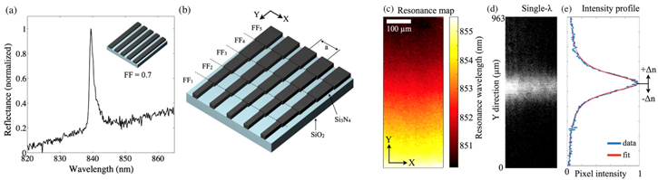
Figure 7. (a) Normal reflectance of a single filling fraction (FF) grating. (b) Schematic of the chirped grating proposed in [119]. The FF is tapered along the grating lines direction. (c) Hyperspectral resonance map showing how the resonance changes spatially along the grating. (d) Brightfield image of the narrow strip lighting up at a specific single wavelength. (e) Intensity profile used to retrieve the pixel position of the line. Reproduced from [119]. CC BY 4.0.
Download figure:
Standard image High-resolution image5.6. Intensity detection
Another way of eliminating the need for a spectrometer is to use an intensity detection scheme. Such a scheme uses a monochromatic source to illuminate the grating, usually an LED [120–122]. The input wavelength (or the grating parameters) is chosen in such a way that the GMR resonance peak stands close to the rising edge of the illumination spectrum (see figure 8(a)). In these conditions, the reflectance is low, because illumination and resonance are detuned. Binding events will shift the resonance to longer wavelengths along the rising edge of the LED, causing the resonance and the illumination to overlap and reflectance to increase. The readout can simply be performed with a detector or a camera. When using the camera, the sensing surface can be spotted with several bioreceptors at different points for different types of molecules to be detected. The simplicity of the configuration has been exploited to make handheld sensors suitable for on-field use and smartphone-based readout.

Figure 8. (a) Illustrates the working principle of the intensity interrogation scheme. The reflectance R increases from R1 to R3 upon binding because of the increased overlap between the GMR resonance and the LED illumination spectrum. (b) is a schematic of the handheld sensor proposed in [123] which is shown in (c). Reproduced with permission from [123], OSA.
Download figure:
Standard image High-resolution imageIn [123], the authors fabricated such a device (shown in figures 8(a) and (b)) and proved it to able to detect three analytes at the same time. Different areas of the gratings are funcionalised drop-wise to detect CD40 ligand antibody at a concentration of 13.5 μg ml−1, EGF antibody (13.5 μg ml−1) and streptavidin (30 μg ml−1). While these values are certainly too high for a diagnostic tool, they estimated a LOD of 24 ng ml−1 for the CD40 and EGF.
5.7. Imaging with GMRs
As already mentioned, GMRs are quasi-guided modes which can efficiently couple to far- field radiation. On resonance, the mode takes the form of a standing wave propagating in the plane of the grating, with a finite penetration depth. If we imagine a point-like perturbation on the surface of the grating, then its influence will extend as far as this penetration depth. This feature allows for the mapping of refractive index distributions over the surface and it can be used for the surface-sensitive imaging of, for example, cells and their adhesion to the sensor.
Probing the mechanisms of cell adhesion to a surface is indeed of great importance for different reasons, such as the monitoring of biofilm formation and growth [124] or the study of the interactions of cell membranes which are fundamental for growth, division, communications or tumour metastasis [125]. Traditional methods for investigating these processes have involved fluorescent dyes or proteins and mainly rely on autofluorescence. Atomic force microscopy (AFM) can also be used for studying cell morphology and mechanical properties. However, AFM does not provide much information about the interaction with the surface as it cannot probe the very interface.
As an alternative, PhC surfaces based on GMRs are completely label-free, as they rely on the refractive index sensing mechanism. The sensing area can be as large as several cm2 making the imaging region limited by the field of view of the camera and the magnification. Tens of cells can be monitored at the same time, increasing throughput. Furthermore, the optical mode penetrates only few hundreds of nanometres into the medium, making it very sensitive to the cellular membrane and its interaction with the surface.
This method of resonant imaging with GMRs or PhCs is also known as photonic crystal enhanced microscopy (PCEM) [98, 126, 127] and data is collected by hyperspectral imaging. The grating is illuminated with a single wavelength which is scanned over a certain range. A standard brightfield image of the surface is taken at each illumination wavelength. The final data set consists of a hyperspectral cube, with each slice corresponding to a 2D brightfield image. The intensity of each pixel is then plotted as a function of the illumination wavelength in order to find the resonance wavelength.
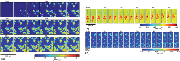
PCEM has been developed and widely explored by Cunningham et al. For example, in [98], they monitored the geometry of cell attachment, which is crucial in stem cell differentiation and cancer cell metastasis. The group were able to follow drug-induced apoptosis over several hours and cell chemotaxis over a few days, which would be impossible with normal staining and fluorescence techniques (see figures 9(a) and (b)). While the spatial resolution is inferior to fluorescence, subcellular details are nevertheless resolved, which may be indicative of a variation of the strength of attachment due to formation of actin bundles and lamellipodia [127]. A comprehensive review of PCEM can be found in [8].
Figure 9. (a) Hyperspectral imaging of mHAT9a cells attaching on the grating surface. The attachment starts as small and rounded areas and then progresses towards larger areas as the cells spread out. The outer boundaries look irregular, consistently with small thin filopodia used by the cells to explore the environment. The sensitivity to surface changes of the GMR makes it ideal for this purpose, as opposed to standard microscopy. (b) Time lapse imaging of cell chemotaxis on the surface. Reproduced from [98] with permission of The Royal Society of Chemistry.
Download figure:
Standard image High-resolution image
5.7.1. Spatial resolution for imaging
Spatial resolution is clearly an important parameter for imaging. Various studies have investigated the resolution limit of resonant imaging based on GMR, i.e. the minimum separation that can be resolved and the minimum feature size that can be reliably reproduced. The limiting factor is the decay length of the mode in the grating plane (Lp), blurring any features smaller than this length.
Typically, the decay length is of the order of a few microns for a standard GMR, but of course it depends on the choice of materials, geometrical parameters and the index contrast induced by the object(s) to be imaged. A careful design is also required because resolution and linewidth of the resonance are inversely related: the smaller the propagation length, the larger the linewidth, which means that the spectral sensitivity will be negatively affected. The propagation length Lp, defined as the distance at which a fraction 1/e of the photons in the mode have been already leaked out, can be expressed as [128]:

where λ is the resonance wavelength and Δλ the FWHM of the resonant peak. This points out a trade-off typical of all physical systems, namely the inverse relation between spatial and spectral resolution: the more spatially confined the mode, the more frequencies contribute. In fact, the main parameter controlling the decay length is the refractive index contrast between ridges and grooves: the higher this contrast, the stronger the reflections at each boundary between grating ridge and cover medium, which inhibits lateral propagation.
For example, in [129] a standard resolution test was placed on a 150 nm thin silicon nitride grating, consisting of an SU-8 pattern. This pattern provides a known distribution of refractive index in the form of different sized and shaped blocks distributed over the surface. Hyperspectral images were recorded in order to determine the minimum feature size and separation that can be resolved. A resolution of 6 μm in the direction perpendicular to the grating grooves (i.e. along the grating vector) and 2 μm along them were demonstrated. This anisotropy arises from the nature of the GMR, which induces oscillations in the direction of the grating vector, in other words, by adding the grating vector to the incoming light. In the perpendicular direction, no such addition of k-vector occurs, and the resolution can be diffraction-limited. 2D-periodic structures, such as an array of air holes etched in a slab, show instead the same limit along both directions. This is expected as the periodic structure imparts momentum in both directions.
In [126], similar values for the spatial resolution are obtained with a slightly different method, i.e. by imaging single TiO2 and gold nanoparticles (NPs) deposited on the resonant grating. The authors analysed the hyperspectral image produced by a single NP by looking at how far it influences the resonance wavelength of neighbouring pixels. Pixels within the decay length of the mode are able to see the particle and show a shift in resonance. The final image is a convolution of this effect, resulting in a maximum wavelength shift centred on the NP and decaying within 3 μm on each side.
5.7.2. Comparison with SPR microscopy (SPRM)
The previous arguments imply that imaging with resonant gratings is perfectly suitable for imaging most types of cells, given their sizes of the order of tens of microns, yet it is challenging to image smaller objects such as single bacteria or even viruses. In this respect, SPRM has shown superior performance. The operational principle of SPRM is very similar, whereby a plasmon wave is excited which has a finite propagation length and which allows to map the intensity of the reflected wave depending on the local refractive index. The key difference, which represents the advantage of SPR for imaging, is that the nature of the plasmon wave allows for higher freedom of tuning the propagation length. For example, for a 47 nm thin layer of gold at a wavelength of 532 nm the lateral propagation of the plasmon is reduced to 200 nm [130, 131]. Basically, it is physically possible to extinguish the SPR within very short lengths (up to very close to the diffraction limit) because of the high level of confinement naturally offered by metals and their absorption. Clearly, the drawback of such a short propagation length is an even broader resonance and a worsening of the overall FOM. GMRs are more limited in this respect because of the very nature of the mode, which consist of a standing wave relying on the index contrast provided by the ridges. A diffraction-limited confinement of a guided mode resonance in such a grating would imply that the standing wave should be excited and extinguished within a length comparable to the period, that is by relying on a single ridge/groove interface. This is clearly not possible. For example, in [126], it is estimated that, for their design, ∼6 reflections are needed to resonantly confine the GMR.
The possibility of tailoring the SPR extinction length to sub-micron dimensions has enabled imaging of single bacteria tethered to the surface via antibodies [132] and even single influenza viruses (about 100 nm in size) [133]. Mapping of proteins within cell membranes and of secretions in the vicinity of the cell body has also been demonstrated [134, 135].
5.8. Integration of PhC slabs with fluorescence
Traditional fluorescence-based techniques are still widely used in many areas of research [136]. Although the use of labels entails increased process time, potential interference with the function of the biomolecules of interest and photobleaching effects, fluorescence-based methods can be very selective, they provide excellent contrast for imaging and they can be sufficiently sensitive to allow the detection of individual molecules [137–139]. In the context of this review, it is worth highlighting that Bragg mirrors [140, 141] and GMR structures [142] can also be used to enhance fluorescence detection by locally enhancing the optical fields at the excitation and/or emission wavelengths.
Critically, one does not want to enhance emission broadband nor in the entire sample volume because of background fluorescence of the bulk solution and other autofluorescence effects. The field enhancement should therefore be localised both spatially and spectrally. The spatial localisation has traditionally been achieved with confocal microscopy [143], light-sheet microscopy [144, 145] or by using two-photon excitation microscopy [146]. Bragg mirrors and GMRs provide this ability by increasing the electric field only very close to the surface [140, 147, 148], similarly to total internal reflection fluorescence microscopy [149].
The second requirement of spectral localisation is easily achieved by resonant photonic structures. The Bragg mirror approach has been shown to enhance both the excitation and emission wavelengths with a total enhancement factor of 10–15 observed, while the GMR approach is particularly well suited to enhancing the fluorescence emission. Because the fluorescence signal can readily couple to GMR modes, the structure additionally acts as an antenna that also increases the extraction efficiency. The net effect is to enhance the SNR and to allow for the detection of extremely low concentrations of analyte. For example, in [150] the authors showed that a 2D GMR grating provided an enhancement factor for the SNR of over 8 compared to a bare glass slide for the detection of the protein TNF-α. This improvement allowed to reach an LOD of 1.6 pg ml−1. The same authors later reported on the application of the same technique to DNA microarrays, where a 10 × better SNR was demonstrated [151].
A similar configuration was used for PCEF (photonic crystal enhanced fluorescence) microscopy. In [152], 3T3 fibroblast cells attached onto a 1D GMR grating are imaged by exploiting the fluorescence enhancement. The cells were stained with two different dyes that selectively attach to their membranes and the nuclei. The grating was designed to support two resonant modes, one at the excitation wavelength of each dye, so that different features of the cells could be probed with the same experiment. The setup also allowed to map the cellular activity in three dimensions because of the different enhancement factor experienced by dyes at different distances from the surface, according to the modelling presented in [147]. Enhancement factors of up to 20 have been achieved.
6. Conclusions and future perspectives
In conclusion, we have considered a range of PhC-based sensing and imaging modalities and compared them to competing methods, particularly to SPR techniques. The main metric we have employed for such a comparison is the widely used FOM defined as the product between the Q factor of the optical resonance and the bulk wavelength sensitivity, so FOM = Q*Sλ. We have highlighted that the link between this FOM and the sensing performance is not trivial. For example, the measurement noise is critical for determining the smallest shift that can be detected and hence the LOD. Differences in the noise characteristics of experimental setups make it difficult to compare devices based on different technologies because experiments are being performed in different, and often unspecified conditions. Thus, the design of a sensor for obtaining a high FOM needs to be accompanied by a careful design of the measurement apparatus in order to fully exploit the potentialities that a high FOM can offer. This critical link is often neglected in the literature.
In the biosensor landscape, the SPR method that was first commercialised by Biacore can certainly be considered as the 'gold standard' that should be used as the main reference point. The Biacore platform is capable of detecting small molecules down to concentrations of the order of ng ml−1, but the device is bulky and expensive, making it suitable only for high-end labs. The goal is therefore to develop cheaper and more compact alternatives that could be used in any lab, yet compete with the SPR performance, or alternatively, to develop novel functionalities that SPR cannot reach.
PhC cavities can perform better in terms of the LOD because of their higher Q factor and correspondingly higher FOM, provided that noise sources are carefully controlled in order to reliably track small shifts of the resonance peak. The main issue with integrated guided-wave optics devices such as PhC cavities is the interfacing difficulty: it is not straightforward to couple light from free-space into a micrometre-scale single mode waveguide, even if grating couplers are used. Many papers focus on the small area that can ultimately be accessed for sensing, but they ignore the fact that bulky apparatus is required to access this small area and/or the fact that active alignment is needed, which immediately restricts the application to a specialist laboratory setting. On the other hand, more recent developments point to novel solutions, e.g. a novel 'flood-exposure' approach that has been demonstrated and that allows coupling from a free-space broadband source to single mode waveguides even in a low-cost setting [88].
Once the coupling difficulty has been taken into account, the small footprint enables integrated devices to perform multiplexed measurements and sensing in small regions. Arrays of PhC cavities can be exploited to multiplex measurements in order to detect tens of analytes in parallel, which is desirable for clinically relevant situations. The simultaneous detection of different biomarkers is often required for increasing the fidelity of the diagnosis. Thanks to their small footprint, photonic probes have also been inserted successfully into living cells while keeping them viable for extended periods of time. This is highly advantageous in comparison to traditional labelling techniques such as ELISA and it is certainly worth exploring for future developments, especially in the context of single cell analysis.
GMR-based devices hold great promise in terms of their ease of interfacing. Based on the quasi-guided nature of these modes, GMRs do not require the focusing of light into wavelength-sized waveguides or cavities. Instead, a collimated light beam is directed onto a relatively large area (up to mm2) while the readout is performed with a simple camera for identifying the brightest pixels. GMRs are also suitable for multiplexing. Different locations on the surface can be funcionalised for the detection of different analytes by using spotting techniques, and all interrogated simultaneously. Non-functionalised areas can then be included on the same chip for providing continuous referencing.
So, what is the best device or configuration for biosensing? There is no simple answer to this question and it really depends on the application. The pros and cons discussed in the previous sections can be summarised as follows:
- •PhC cavities can be extremely sensitive and offer very low limits of detection, but they are difficult to manufacture and to measure. The more the light is confined to tiny cavities, the more difficult it is to couple in and out. Cavities are suitable for more fundamental studies aimed at pushing the limit of light-biological matter interaction and at investigating fundamental mechanisms of molecular adsorption and binding kinetics and affinity, for example. They are not suitable, however, for applications in the field or for high-throughput experiments. Fabrication is neither easy nor low-cost. However, they offer good capabilities of multiplexing due to their reduced footprint, as well as the possibility of interrogating very small volumes inside single cells.
- •GMR structures show modest sensitivities and limits of detection, but they are inherently more practical and easier to use. The nature of the leaky modes employed in GMRs makes them very easy to interface. The sensing area can be very large, up to several cm2, or very small, down to a few micrometres. It is possible to fabricate large sensors by nanoimprint technology, thereby increasing throughput and reducing cost. GMRs are extremely suitable for on-field application and hold great promises for POC sensors. Importantly, imaging is an intrinsic ability given that the GMR modes have a finite propagation length. However, their modest LOD may preclude their applicability from many clinically-relevant concentrations of biomarkers, especially those that have to be detected in very low concentrations. The performance of GMRs can be dramatically enhanced e.g. by implementing phase detection schemes, which is an active area of research.
- •In terms of the FOM defined as Q*Sλ, we can group devices in two categories. The first category comprises PhC cavities and microring resonators, which show similar values of the FOM that are amongst the highest among all optical biosensors. Between the two, the ring configuration emerges as the most widely employed for biosensing, thanks to the less stringent fabrication constraints and the availability of the MaverickTM platform commercialised by Genalyte. SPR and GMR-based devices belong to a second category, showing more modest values of the FOM because of the limited Q. In this case, SPR is preferred in high-end labs because of the commercially established Biacore system and the convenience of having a standard and tested device for conducting experiments. In comparison, GMR-based devices do not yet share a big portion of the biosensor market and community, but they have great potential in the low-cost market because of their simplicity and ease of interfacing.
Despite all the challenges yet to be addressed, the field of optical biosensors poses exciting and stimulating tasks. Original and functional solutions must lie at the boundaries between different disciplines, which makes them one of the best example to epitomise the value of interdisciplinarity.
Acknowledgments
GP and TFK acknowledge funding from the EPSRC Programme Grant EP/P030017/1 'Resonant and shaped photonics'. TFK acknowledges the Royal Society Wolfson Research Merit Award Scheme.