An iterative method for near-field Fresnel region polychromatic phase contrast imaging

The speed at which x-ray phase contrast imaging [1] data can be collected may be dependent on the x-ray source that is employed. More efficient use of polychromatic light sources can be achieved if the energy dependent effects on image formation can be included in image reconstruction algorithms. By using more of the available flux the exposure time can be significantly reduced, which may allow quantitative imaging of dynamic systems.

At the expense of higher computational cost, iterative techniques for monochromatic propagation-based x-ray phase contrast offer the benefit of being able to operate in regimes where analytical techniques fail [2].

Far-field iterative techniques, such as coherent diffractive imaging (CDI) [3], have been adapted to be compatiable with polychromatic sources [4, 5]. Collectively, these polychromatic techniques are known as 'polyCDI'. However, to the best of our knowledge, there has been no demonstration of polyCDI techniques in the near-field.

In this work, we demonstrate an iterative algorithm that extends the ideas of polyCDI into the near-field and provides an experimental demonstration of its utility using a broad spectrum from a synchrotron bending magnet source. This algorithm was developed for use with objects of uniform composition and has the advantage that it allows the thickness of the object to be readily recovered. The algorithm can be employed for any sufficiently well characterised polychromatic light source, including those typically found in laboratories.

A finite polychromatic spectrum can be represented as a sum of components that each have a discrete wavelength $({\lambda }_{1},{\lambda }_{2},\ldots ,{\lambda }_{n})$ and appropriate weighting, ${\xi }_{\lambda }$, for each wavelength. The number, n, of discrete wavelengths will determine how accurately the polychromatic spectrum is described.

While the thickness is invariant with wavelength, the experimental estimations for different wavelengths can be averaged to obtain a more accurate result. As such, the calculated sample thickness for a particular wavelength, ${{\boldsymbol{t}}}_{\lambda }$, is defined as

$$\begin{eqnarray}&&{{\boldsymbol{t}}}_{\lambda }=\left|\displaystyle \frac{\mathrm{ln}{{\boldsymbol{T}}}_{\lambda }}{-{k}_{\lambda }({\beta }_{\lambda }+{\rm{i}}{\delta }_{\lambda })}\right|,\end{eqnarray} \tag{ 1 }$$

where ${\beta }_{\lambda }$ and ${\delta }_{\lambda }$ represent the real and imaginary components of the sample's refractive index for a particular wavelength, λ. The wave number is ${k}_{\lambda }=\tfrac{2\pi }{\lambda }$ and ${{\boldsymbol{T}}}_{\lambda }$ is the complex transmission function for a given wavelength.

The sample thickness, ${\boldsymbol{t}}$, can be defined as

$$\begin{eqnarray}&&{\boldsymbol{t}}=\displaystyle \sum _{\lambda }{{\boldsymbol{t}}}_{\lambda }{\xi }_{\lambda }.\end{eqnarray} \tag{ 2 }$$

Using the operator notation commonly used to describe CDI algorithms [6–8], we can describe how the thickness can be explicitly included in the reconstruction algorithm:

$$\begin{eqnarray}&&{{\boldsymbol{\psi }}}_{\lambda }^{{}^{i+1}}={\pi }_{s\lambda }{\pi }_{m\lambda }{{\boldsymbol{\psi }}}_{\lambda }^{i},\end{eqnarray} \tag{ 3 }$$

where ${{\boldsymbol{\psi }}}_{\lambda }$ is the object's exit surface wave at wavelength λ for the $i{\rm{t}}{\rm{h}}$ iteration. The exit surface wave is defined by the transmission function ${{\boldsymbol{T}}}_{\lambda }$ and the incident wavefield, ${{{\boldsymbol{\psi }}}_{{\bf{0}}}}_{\lambda }$, as

$$\begin{eqnarray}&&{{\boldsymbol{\psi }}}_{\lambda }={{{\boldsymbol{\psi }}}_{{\bf{0}}}}_{\lambda }{{\boldsymbol{T}}}_{\lambda }.\end{eqnarray} \tag{ 4 }$$

The modulus constraint, ${\pi }_{m\lambda }$, is defined as

$$\begin{eqnarray}&&{\pi }_{m\lambda }={P}_{\lambda }^{-1}{\hat{\pi }}_{m\lambda }{P}_{\lambda }\end{eqnarray} \tag{ 5 }$$

$$\begin{eqnarray}&&=\,{P}_{\lambda }^{-1}\displaystyle \frac{{\hat{{\boldsymbol{\psi }}}}_{\lambda }}{| {\hat{{\boldsymbol{\psi }}}}_{\lambda }| }\sqrt{{\boldsymbol{I}}}{P}_{\lambda },\end{eqnarray} \tag{ 6 }$$

where for each wavelength ${P}_{\lambda }$ and ${P}_{\lambda }^{-1}$ represent the forward and reverse propagation operators and ${\hat{{\boldsymbol{\psi }}}}_{\lambda }$ is the propagated detector wavefield and ${\boldsymbol{I}}$ is the measured detector intensity.

Application of the modulus constraint to each wavefield gives an estimate for the object exit wavefield. Combining equations (4), (1) and (2) gives an estimate for the object thickness, ${{\boldsymbol{t}}}^{\prime }$, taking into account all wavelengths in the summation. To obtain the next iterative for the thickness the support constraint can be applied

$$\begin{eqnarray}{\pi }_{s}{{\boldsymbol{t}}}^{\prime }=\begin{array}{cc}{{\boldsymbol{t}}}^{\prime } & {\boldsymbol{r}}\in {\boldsymbol{S}}\\ 0 & {\boldsymbol{r}}\notin {\boldsymbol{S}},\end{array}\end{eqnarray} \tag{ 7 }$$

where ${\boldsymbol{r}}=(x,y)$ is a two-dimensional position vector and ${\boldsymbol{S}}$ is the area of the support constraint, and ${\boldsymbol{S}}$ is chosen to satisfy the sampling constraints [9]. The next iteration for each exit wavefield of interest can than be obtained by applying equation (4).

The convergence of a solution is monitored via the ${\chi }^{2}$ difference between the detector plane intensity estimated at the current iteration compared to the measured intensity. The ${\chi }^{2}$ metric is given by

$$\begin{eqnarray}&&{({\chi }^{2})}^{i}=\displaystyle \frac{{\sum }_{n=0}^{N-1}{({\sum }_{\lambda }({{\boldsymbol{\psi }}}_{\lambda n}^{i* }{{\boldsymbol{\psi }}}_{\lambda n}^{i}{\xi }_{\lambda })-{{\boldsymbol{I}}}_{n})}^{2}}{{\sum }_{n=0}^{N-1}{{\boldsymbol{I}}}_{n}},\end{eqnarray} \tag{ 8 }$$

where the sum is performed over all N pixels in the image.

In simulations in which the object thickness is known, convergence is monitored via the ${\chi }^{2}$ between the recovered object thickness and the known object thickness in each pixel. This error metric is expressed as

$$\begin{eqnarray}&&{({\chi }_{{\rm{sample}}}^{2})}^{i}=\displaystyle \frac{{\sum }_{n\in {\boldsymbol{S}}}{({{\boldsymbol{t}}}_{n}^{^{\prime} i}-{{\boldsymbol{t}}}_{n})}^{2}}{{\sum }_{n\in {\boldsymbol{S}}}{{\boldsymbol{t}}}_{n}}.\end{eqnarray} \tag{ 9 }$$

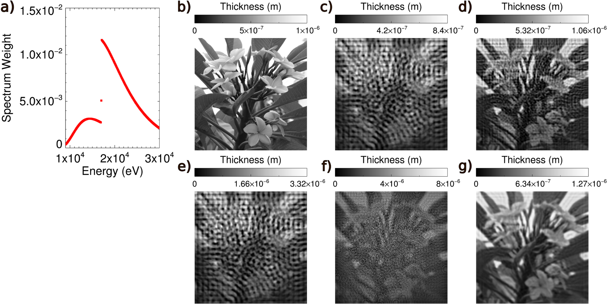
The outcomes of a numerical simulation demonstrating the effectiveness of our method in obtaining a quantitative reconstruction for an object in the near-field for a spectrum defined over the range 9 and 30 keV with the energy binned at 100 eV intervals is shown in figure 1(a). The spectrum is modelled on Diamond's B16 ideal bending magnet, with an 500 μm thick Al filter and a YAG:Ce 35 μm scintillator transmission factored in. The test object, shown in figure 1(b), has a thickness from 0 (black) to 1 μm (white) and is made of gold with a uniform composition. A density of 13.8 g cm⁻³ was used when calculating the appropriate β and δ values. A point source was simulated to be placed 0.76 m from the sample, z₁, while the detector was simulated to be 0.24 m away from the sample, z₂. A detector pixel size of 450 nm was used, resulting in a sample pixel size of 342 nm. The oversampled image contained 710 × 710 pixels, with the sample occupying 345 × 345 pixels,the loose support constraint used was 355 × 355 pixels and centred over the sample. The Fresnel propagator in its convolution form [1, 10] was used to propagate between the sample and detector planes. This propagator is ideal for the present situation as it accurately accounts for phase curvature in the wave from a point source and the output pixel size is not wavelength dependent [10]. Iterative reconstructions using the lowest, peak, weighted average and highest energy (and their associated β and δ values) are shown in figures 1(c)–(f). Figure 1(g) is the result obtained using our method and shows how the algorithm can reconstruct the object with significantly less artefacts.

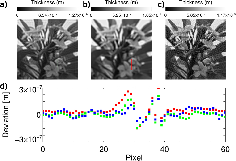
Zoom In Zoom Out Reset image size

Our method of reconstruction was compared to polychromatic versions of the transport of intensity equation (TIE) [11] and contrast transfer function (CTF) [12]. The TIE reconstruction used values of an energy, β and δ of 19.137 keV, $6.34\times {10}^{-7}$ and $6.44\times {10}^{-6}$ respectively. The same spectrum and values of β and δ that were used for the iterative method were used for the CTF reconstruction and a Tikhonov regularisation [13] of $\alpha =0.03$ was applied. The results are shown in figures 2(a)–(c) and a line profile quantitatively comparing the thickness reconstruction is shown in 2(d). The resultant ${\chi }^{2}$ errors for thickness for each method are shown in table 1 and demonstrate that, in this geometry, the quantitative thickness reconstruction for the iterative method is comparable to the polychromatic CTF method. However, figure 3 shows that if source blur and Gaussian noise are applied to the phase contrast image, the iterative method is able to provide a reconstruction that is better both qualitatively and quantitatively than the polychromatic analytical methods.

Zoom In Zoom Out Reset image size

Zoom In Zoom Out Reset image size

Table 1.  Polychromatic iterative, TIE and CTF using the sample plane ${\chi }^{2}$ metric for the reconstructions presented in figure 2. The metric is calculated using equation (9) in the region where the sample is present.

Polychromatic algorithm	No source blur and noise ${\chi }^{2}$	Source blur and noise ${\chi }^{2}$
Iterative	1.71 × 10−8	2.17 × 10−8
TIE [11]	2.91 × 10−8	3.26 × 10−8
CTF [12]	1.11 × 10−8	1.43 × 10−7

The computational cost of our method will be dependent on the width of the source spectrum, the energy binning size employed and the efficiency of the computational programming (for example parallel programming and the choice of programming language itself could be used to optimise the process compared to the implentation of IDL [14] that was used here). The analytical nature of the polychromatic TIE algortithm [11] means this method will always allow faster reconstructions than the polychromatic CTF method [12] and the iterative approach we have described here. However, figure 2 and table 1 show qualitatively and quantitatively that the polychromatic CTF and iterative methods can provide a better quality reconstruction than the polychromatic TIE. Furthermore, as we have previously demonstrated [2], an appropriate choice of propagator allows the iterative method to operate in regions where the TIE and CTF begin to fail.

Diamond Light Source's B16 bending magnet test beamline [15] was used to perform a proof-of-concept experiment. A white beam in-line phase imaging geometry was employed, as shown in figure 4.

Zoom In Zoom Out Reset image size

For the propagation between the sample and detector planes, we used used the Fresnel propagator in its convolution form. To satisfy the propagator requirement [10], a 500 μm Al filter was was placed upstream of the Kirkpatrick–Baez (KB) mirror. This filter removed the components of the spectrum below 9 keV. The focus of the KB mirror was used to create a 'point source' for the phase contrast imaging experiment with a vertical and horizontal full width half maximum of 0.607 and 0.837 μm respectively. The sample was placed 0.76 m away from the point source, z₁, while the detector was placed 0.24 m after the sample, z₂.

A YAG:Ce 35 μm thick scintillator was used with a 20× objective lens and a cooled 14 bit charge-coupled device camera. The resultant CCD pixel size was 450 nm, giving an effective pixel size of 342 nm in the sample plane. Two hundred phase contrast and white-field images were acquired, with each image having an exposure time of 2 s.

The area recorded on the detector contained the phase contrast image of the object, which was made from Au deposited onto a ${\mathrm{Si}}_{3}{{\rm{N}}}_{4}$ window. The object occupied an area of 105 μm × 105 μm of the window. As seen in figure 5(a), the sample thickness was 350, 650 and 1000 nm in different regions (blue, green and red shaded regions in figure 5 respectively).

Zoom In Zoom Out Reset image size

This experimental geometry is valid for the iterative and TIE methods. For particular energies in some regions, the phase condition for the CTF is violated, but simulation suggested this was unlikely to cause significant artefacts.

To account for non-uniformity in the illuminating beam, the combined phase contrast image was normalised by dividing the combined white-field image on a pixel-by-pixel basis. Some instability in the illuminating beam meant that the resulting image was still not uniform in areas where uniformity was expected. While this limited the accuracy of the recovered thickness, the data obtained is of sufficient quality to provide a proof-of-principle comparison between our iterative method and the polychromatic TIE and CTF methods.

The β and δ values required for our method were obtained by interpolating reference data from Henke et al [16] over the range 9–30 keV in bins of 100 eV. We have previously calculated the density of the Au sample to be 13.8 g cm⁻³ rather than bulk density [2]. Accordingly, this value was used when calculating the β and δ values.

The bending magnet spectrum defined at 100 eV intervals over the range 9–30 keV with absorption effects of the Al filter and YAG:Ce scintillator is shown in figure 1(a). The bending magnet emission will extend beyond 30 keV, but we did not include these high energy components as under experimental conditions they provided minimal phase contrast fringing. Our method using the Fresnel propagator in its convolution form was applied to the normalised phase contrast image. A tight support and 1000 iterations were used in the reconstruction. The detector plane error metric stabilised after the 300 iteration mark.

Our result was compared to polychromatic TIE [11] and CTF [12] reconstructions (figure 6). The TIE reconstruction employed an energy, β and δ of 19.137 keV, $6.34\times {10}^{-7}$, $6.44\times {10}^{-6}$ respectively. The CTF reconstruction used the same spectrum, β and δ as our iterative method and applied a Tikhonov regularisation [13] of $\alpha =0.047$. The mean of the region outside of the sample was used to determine the zero thickness offset for each of TIE and CTF reconstitutions. The Tikhonov regularisation value was deliberately chosen to give the expected value for the 1000 nm region. While this would not be possible for thickness under experimental conditions with no reference available, it allows us to perform a comparison here under conditions most favourable to the existing technique.

Zoom In Zoom Out Reset image size

To the eye, the quality of the recovered thickness maps for our method and the polychromatic TIE and CTF are similar. The polychromatic iterative method appears less susceptible to missing information in the phase contrast image when compared to the monochromatic iterative phase contrast method [2]. For example, the 'cross-hatching' artefact seen in our monochromatic iterative phase contrast method is notably absent. This may be explained in terms of a phase diversity argument [17]. For each energy, source blurring and noise cause a loss of information in the phase contrast image and a monochromatic reconstruction would still suffer from the cross-hatching artefact. However, in the polychromatic data, this effect is different for each energy bin and the combination of energies, via equation (4), creates an averaging effect where the object is reinforced and the artefacts are smoothed out.

The quantitative thickness results are shown in figure 7. It can be seen that our iterative approach performs as well as the CTF method and both perform slightly better than the TIE approach. However, it should be noted that our iterative approach can operate reliably in regimes where the validity conditions for the CTF and TIE are violated to the extent that they become inaccurate [2]. The combination of extended validity and the 'phase diversity' effect means that our iterative method offers flexibility in the phase contrast image reconstruction process, potentially allowing an optimisation of reconstruction that is not possible with direct analytical approaches. In all cases, the 650 nm region (green) provides results that are poorer when compared to the 350 and 1000 nm regions. This result is largely due time variability in the beam, which causes non-uniformity in the background that affects this part of the image. Figure 8 shows this effect where two images of the same region show variation in the 650 nm (green) region.

Zoom In Zoom Out Reset image size

Zoom In Zoom Out Reset image size

This work has concerned itself with algorithm development using a proof of principle demonstration of broadband phase contrast imaging using a simple homogeneous sample. It is worth noting that x-ray imaging using similar iterative techniques has proven itself capable of high-resolution imaging under a wide range of conditions [5, 18–22]. These demonstrations show that with optimised experimental conditions our algorithm also has the capability of providing quantitative and high resolution imaging in regimes where analytical techniques begin to break down.

A propagation-based polychromatic iterative phase contrast imaging technique has been experimentally demonstrated in the near-field Fresnel region. The technique was shown to allow quantitative determination of the thickness of a sample. The results obtained were comparable to the analytical polychromatic TIE and CTF methods.

Under geometrical, noise and source blur conditions that would render both the polychromatic TIE and CTF methods inaccurate, we have shown in simulation that the iterative method can provide high quality and quantitative results.

The quantitative accuracy of the images obtained using our technique suggests that it could be extended to phase contrast imaging using laboratory x-ray sources.

The authors acknowledge the support of the Australian Research Council through the Centres of Excellence for Coherent x-ray Science and Advanced Molecular Imaging. We thank Diamond Light Source for access to beamline B16 (proposal number MT9625) that contributed to the results presented here.

This work was performed in part at the Melbourne Centre for Nanofabrication (MCN) in the Victorian Node of the Australian National Fabrication Facility (ANFF).