

Abstract
This work presents a comparison between the PTT-X (extended Phan-Thien and Tanner (PTT)) and the generalised PTT (gPTT) viscoelastic models. The PTT-X model was derived based on a combination of reptation and network theories, allowing in this way a microstructural justification for the kernel function. The gPTT model is based on the network theory, with an empirical kernel function for the rate of destruction of junctions, that proved to be effective fitting experimental rheological data for polymer melts and solutions. A review on the background of both models is provided and the two models are then compared considering simple flows. This comparison allows one to attribute in some way a microstructural nature to the parameters involved in the gPTT model. Also, a new analytical solution is derived for the Poiseuille flow of the PTT-X model.
Export citation and abstract BibTeX RIS

Original content from this work may be used under the terms of the Creative Commons Attribution 4.0 license. Any further distribution of this work must maintain attribution to the author(s) and the title of the work, journal citation and DOI.
Recommended by Dr Stefan Llewellyn Smith
1. Introduction
In 1932 and 1940, Busse (1932) and Treloar (1940) claimed that elasticity of polymers comes from temporary entanglements between chains. Green and Tobolsky (1946), Lodge (1956)and Yamamoto (1956) presented the idea of entanglements in melts as temporary cross links. In 1952, Bueche (1952) introduced the concept of entanglement friction, that is, as one chain slides around the other chains (with snaking circulation movements), it will create some friction on the chains osculating that chain. In 1953, Rouse (1953), Rouse and Sittel (1953)developed a model for linear polymers (known as the Rouse model). The model consists of beads of infinite modulus connected to each other by springs of no mass and volume. In 1967, Edwards (1967a, 1967b)presented the tube model. The idea is that each polymer chain is surrounded by a tube that mimics the restrictions imposed by the surrounding chains. The surrounding chains will restrict the transverse movement of a polymer chain. In 1971, de Gennes (1971) introduced the concept of polymer reptation (reptation suggests the movement of entangled polymer chains as being analogous to snakes slithering through one another). Entangled chains move along the confining tubes, and, the chain is free to move among fixed obstacles but cannot cross any fixed obstacle. Later, in 1978, Doi and Edwards (1978a, 1978b)refined the theory of reptation and applied the reptation model to the rheology of entangled polymers.
Nowadays, the network (Lodge 1956, Yamamoto 1956) and reptation theories are still being used, and several constitutive equations found in the literature are based on such theories. Of course these theories have some drawbacks, and with the advances in technological developments, experimental works reveal their weaknesses. For example, in a recent work (2017) by Wang (2017) they did not observe experimentally the fast chain retraction process after deformation (followed by a slow orientation through a reptation mechanism), as predicted by the classical tube theory of Doi and Edwards. Since no perfect theory has yet been developed, such models are of great importance for understanding and predicting the polymeric flow behaviour.
The interested reader can find a review on tube model based constitutive equations for polydisperse linear and longchain branched polymer melts in the work by Narimissa and Wagner (2019).
The main objective of this work is to relate the generalised PTT model (Ferrás et al 2019a, 2019b, 2019c) to the PTT-X model (Tanner and Nasseri 2003), providing some microstructural explanation for the empirical kernel given by the Mittag–Leffler function in the new gPTT model. Also, we compare the fitting capabilities of the gPTT and the PTT-X models.
The molecular origin of the parameters in viscoelastic constitutive equations is important because it provides insight into the underlying physical mechanisms that govern the behaviour of the material. By understanding the molecular mechanisms, we can make predictions about how the material will behave under different conditions, and we can design materials with specific properties tailored to particular applications.
For example, knowing the molecular origin of the parameters in a viscoelastic constitutive equation can help us design materials that exhibit specific viscoelastic behaviours, such as strain-rate sensitivity, stress relaxation, or creep. This knowledge can also help us understand the response of materials to external stimuli, such as temperature, pressure, or chemical environment.
Moreover, understanding the molecular origin of the parameters can also help us to develop more accurate and predictive models. Inaccurate or imprecise models can lead to errors in the design and manufacture of materials and can result in costly failures or suboptimal performance.
By gaining knowledge on the relation between the gPTT model and reptation theory, we can therefore further develop the model and better understand its limitations and application in specific viscoelastic fluids.
The paper is organised as follows: this introduction is followed by section 2, where the governing equations are presented. In section 3 the differences between the different kernel functions are explored. Section 4 is devoted to steady flows (Poiseuille and Couette flows), where a new analytical solution for the PTT-X model is derived. The closure of the paper follows in section 5.
2. Formulation and constitutive equations
Melts such as low density polyethylene (LDPE) have multiple, irregularly spaced, long side branches. They show strain-hardening phenomenon (transient viscosity after start-up of flow) in uniaxial extensional flow that differs qualitatively from the behaviour of unbranched melts. In shearing flows, the LDPE shows a strain-softening similar to ordinary un-branched melts (these melts show predominantly strain-softening characteristics in both shear and extensional flows). Therefore, such materials caught the attention of researchers and constitutive models started being developed, namely, the pom-pom model. This model is based on a tube model (as for entangled linear polymers), it assumes an idealised molecule (pom-pom), and is made of a single backbone with multiple branches at each end.
The pom-pom model was introduced by Bishko et al (1997), McLeish and Larson (1998)and it was extended by Verbeeten et al (2001) (it was renamed XPP model), introducing a non-zero second normal stress difference in shear, removing the discontinuities in steady state elongation and the unboundedness of the orientation equation for high strain rates.
The XPP model is given by

with  being the usual upper-convected time derivative,

and F being of the form
where  is the trace of the stress tensor,
I
is the identity tensor,
τ
is the stress tensor,
D
is the rate of deformation tensor,
L
is the velocity gradient (
is the trace of the stress tensor,
I
is the identity tensor,
τ
is the stress tensor,
D
is the rate of deformation tensor,
L
is the velocity gradient ( with
with  ), q is the number of arms of the branched molecule, λ is the usual linear relaxation time, λb
is a time constant for stretch, G0 is the shear modulus and α is the parameter from the Giesekus model (a mobility factor, whose origin is associated with anisotropic Brownian motion and/or anisotropic hydrodynamic drag of the polymer molecules (Larson 1988)).
), q is the number of arms of the branched molecule, λ is the usual linear relaxation time, λb
is a time constant for stretch, G0 is the shear modulus and α is the parameter from the Giesekus model (a mobility factor, whose origin is associated with anisotropic Brownian motion and/or anisotropic hydrodynamic drag of the polymer molecules (Larson 1988)).
As we will explain later, the XPP model is related to the PTT-X model (Tanner and Nasseri 2003), which is given by

The PTT-X model is based on a general network theory (a network with the destruction and formation of new networks), but now incorporates the microstructural knowledge obtained from the reptation theory, through the inclusion of function  . Note that the PTT-X model ignores the terms
  (Giesekus term that was introduced in the XPP model to obtain a second normal stress difference) and
  in equation (1). In reality what happens is that all forms of the PTT model consider that the destruction and creation functions are identical, which results in that term disappearing.
The PTT-X model predicts similar results as the XPP model for high elongation rates (the Giesekus term  has a small influence), but, the results differ for high shear rates, where the rate of creation of junctions plays an important role (the Giesekus term also has some influence on the results).
This model will be compared with the exponential (Phan-Thien 1978) and generalised (Ferrás et al 2019b, 2019c) PTT models (see also Phan-Thien and Tanner 1977), where the function of the trace of the stress tensor is given by (for the gPTT model)

Note that  in equation (5) is the Gamma function defined via a convergent improper integral

The prefactor  is used to ensure that
  , for all choices of β. The Mittag–Leffler function is defined by

with α, β real and positive (note that since we will not consider the Giesekus term, the parameter α is now used in the Mittag–Leffler function, with no connection to the Giesekus model). When  , the Mittag–Leffler function reduces to the exponential function, and we obtain the exponential PTT model with the kernel
  (ε is a dimensionless parameter of order 0.01 for the exponential PTT model).
When β = 1 the original one-parameter Mittag–Leffler function, Eα , is obtained.
3. Kernel functions
The kernel function plays a critical role in these models by providing a mathematical description of the viscoelastic behaviour of the polymer chains and allowing the model to accurately predict the mechanical response of the material under different loading conditions (different deformations).
In the previous section we presented three kernel functions for the PTT model. These are given by equations (3) and (5) for the PTT-X and gPTT models (respectively) and by  for the exponential version (this exponential form is obtained for the gPTT model with
  ). In order to see the differences between these kernel functions and for ease of understanding we will consider a simpler version of the gPTT model, with the kernel given by

Figure 1(a) shows the plots obtained considering η = 50 Pa·s, λ = 0.003 s,  s, ε = 0.01 and q = 6. For the gPTT model we assume β = 1 and use two different values of α (0.35 and 0.4). These parameters represent a general viscoelastic fluid and were chosen only to facilitate the comparison between the PTT-X and gPTT models.

Figure 1. (a) Variation of the kernel function  with the trace of the stress tensor for the exponential (gPTT with
  ), generalised PTT and extended PTT model. For the gPTT model we consider two cases with α = 0.35 and 0.4. (b) The PTT-X kernel function for different values of q (the number of arms in the backbone ends). In all cases we assume η = 50 Pa·s, λ = 0.003 s,
  s, ε = 0.01.
Download figure:
Standard image High-resolution imageIt is obvious that the exponential model presents a slower growth, through the kernel function used therein, when compared to the kernel function of the gPTT and PTT-X models. Note that the PTT-X kernel presents a different growth than the one shown by the gPTT. Due to the existence of a function multiplying the exponential function, the PTT-X kernel changes its curvature as the trace of the stress tensor increases (specially for low values of  ). For higher values of
  the PTT-X kernel shows an almost linear behaviour.
In order to perform a better analysis and comparison of the results, different parameters will be considered next.
The growth of  is much more pronounced for the gPTT kernel, and the lower the α the higher the rate of destruction of junctions (Ferrás et al
2019b).
is much more pronounced for the gPTT kernel, and the lower the α the higher the rate of destruction of junctions (Ferrás et al
2019b).
Figure 1(b) shows the PTT-X kernel for different number of arms (q). As we increase the number of arms of the molecule, the rate of increase of  becomes smaller because q is directly related to the stretch and relaxation of the fluid (Verbeeten et al
2001). The quantity
becomes smaller because q is directly related to the stretch and relaxation of the fluid (Verbeeten et al
2001). The quantity  can also be seen as a measure of the influence of the surrounding polymer chains on the backbone tube stretch (Verbeeten et al
2001).
can also be seen as a measure of the influence of the surrounding polymer chains on the backbone tube stretch (Verbeeten et al
2001).
It should be remarked that for high  , the exponential behaviour of the PTT-X kernel will stand out (when compared to the term
  ), leading to:
We will now compare the gPTT and PTT-X kernels. We consider different values of q and fit the gPTT kernel function to the PTT-X kernel by tuning the α and ε parameters. All other parameters are kept constant.
We consider  Pa·s, λ = 0.003 s,
  s and β = 1. We also measure the error, the maximum relative error in percentage (relative difference between the results obtained with the gPTT and PTT -X models, where PTT-X is the reference model). Figure 2 shows the cases: (a) q = 1, ε = 1.8, α = 2.1, (b) q = 2, ε = 5.15, α = 3.1, (c) q = 3, ε = 94, α = 5.2, (d) q = 5, ε = 385, α = 6.2.

Figure 2. Variation of the kernel function  with the trace of the stress tensor for the generalised and extended PTT model. We consider η = 1000 Pa·s, λ = 0.003 s,
  s and β = 1. the error stand for the maximum relative error, in percentage. (a) q = 1, ε = 1.8, α = 2.1, (b) q = 2, ε = 5.15, α = 3.1, (c) q = 3, ε = 94, α = 5.2, (d) q = 5, ε = 385, α = 6.2. The error stands for the maximum relative difference between the two models.
Download figure:
Standard image High-resolution imageWe observe that increasing both α and ε is equivalent to an increase of the number of arms, q, of the molecule. It should be remarked that as the number of arms increases the ability of the gPTT model to mimic the PTT-X kernel behaviour deteriorates. The reason is the following. If we calculate the second derivative of the PTT-X kernel we observe that for lower values of  the kernel is concave and for higher values is convex. This behaviour cannot be achieved by the Mittag–Leffler function, which is used in the kernel function for the gPTT model.
In the Network theory this means (PTT-X kernel behavior) that the rate of destruction of junctions is high for low values of the mean square displacement of the junction's end-to-end vectors (the trace of the stress tensor,  ) (Tanner and Nasseri 2003), then the rate decreases, and it increases again for higher values of
  . Although this phenomenon is not well captured by the gPTT kernel, this does not mean that one model is better than the other. This behaviour may change depending on the type of viscoelastic fluid being studied.
We may therefore argue that up to q = 5 the increase of the α and ε parameters in the gPTT model leads to a response analogous to an increase in the number of arms of the molecule.
The uniqueness of  is difficult to prove in general, but because of the different influences of α and ε on the final solution, we have observed numerically that for the ranges of
  considered in this work, if other
  exist, they are very similar (and they retain the monotonic behaviour). These other solutions may come from other local minima.
4. Steady Couette and Poiseuille flow of a PTT-X fluid
The equations governing the flow of an isothermal viscoelastic fluid are the continuity,

and the momentum equation

together with the constitutive equation, which, for this case is given by equation (4), and is now rewritten considering  as the elastic modulus G0 of the polymeric network (in the absence of a solvent) under equilibrium conditions:

Here,  represents the material derivative given by
  , p is the pressure and ρ the mass density.
4.1. Simple shear flow
Here we compare the generalised Phan-Thien–Tanner (equation (12) with the function of trace of the stress tensor given by equation (5)) and the PTT-X versions of the PTT model. Note that we consider the PTT models in the particular case of affine motion and without the presence of a Newtonian solvent.
To compare these models we study the dimensionless material properties in steady shear flow of the two versions of the PTT model, considering different values of α, ε, λb and q.
The material functions can be obtained considering a steady-state Couette flow in the x-direction,  , where
  is the shear rate. For this flow, the constitutive equation reduces to
From the system of equation (13),  and applying some algebra to the first two equations (dividing the first equation by the second), a relation between the shear stress and the normal stress is obtained,

We can also obtain the viscometric material functions: the steady shear viscosity,  , the first normal stress coefficient,
  , and the second normal stress coefficient,
  , that are given by


The second normal stress coefficient is null,  , so, we only need to find
  and
and  . Therefore, manipulating the second equation of the system of equation (13) we get

The dimensionless expression for the steady shear viscosity becomes

and the dimensionless first normal stress coefficient is given by

To obtain the material function we need to solve the non-linear system of equations (equation (13)), which can be written in terms of τxx in the non-linear form as

Giving values to  , we can find
  using equation (21). Then, the function
  is directly calculated, allowing us to obtain the material functions given by equations (19) and (20). Note that the PTT-X kernel does not make use of ε.
Figure 3 presents the dimensionless material properties for the steady-state Couette flow of a PTT model (exponential (gPTT model with  ), gPTT and PTT-X). In figures 3(a) and (b) we show the influence of the number of arms (q) and the relaxation time ratio (
 ) on the shear thinning viscosity. In figure 3(a) we set
  and vary q. We observe that the increase in the number of arms leads to a less thinning viscosity. The increase in q leads to a stronger entanglement and therefore a higher shear rate is needed to obtain the same thinning viscosity of a fluid with a lower number of arms.
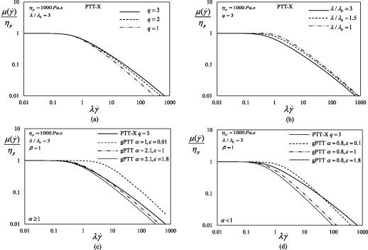
Figure 3. Dimensionless material properties in steady-state Couette flow for the gPTT, exponential (gPTT with  ) and PTT-X models (without solvent viscosity). β = 1 in all cases. Figures (a) and (b) show the influence of the number of arms (q) and the relaxation time ratio (
 ) on the shear thinning viscosity of a PTT-X model. Figures (c) and (d) show a comparison between the PTT-X and the gPTT models.
Download figure:
Standard image High-resolution imageThe variation of  (figure 3(b)) will also affect the thinning behaviour, as expected. It should be remarked that λ was kept constant and only λb
(the time constant for the stretch of the molecule) was varied. Decreasing the relaxation ratio, the shear viscosity thinning effect is only observed for higher values of
(figure 3(b)) will also affect the thinning behaviour, as expected. It should be remarked that λ was kept constant and only λb
(the time constant for the stretch of the molecule) was varied. Decreasing the relaxation ratio, the shear viscosity thinning effect is only observed for higher values of  , and steeper slopes are obtained for a smaller relaxation ratio. The stretch relaxation time is influencing the break point where the viscosity leaves the Newtonian plateau. A higher stretch relaxation time leads to a decrease in the ability of the fluid to flow, and therefore a higher viscosity is observed at higher shear rates. It is interesting to note that for the case of a high break point, the thinning is stronger.
In order to compare the PTT-X to the gPTT model, we have considered different values of ε and α (figures 3(c) and (d)). We set β = 1 in all cases.
Figure 3(c) shows the shear thinning viscosity obtained for the exponential, gPTT (α > 1) and PTT-X models. The exponential model shows a higher break point, when compared to the other two models. It also presents a stronger thinning effect when compared to the PTT-X model.
When it comes to the gPTT model, we have considered two cases, the one that gives a similar behaviour to PTT-X kernel with q = 3, given by α = 2.1 and ε = 1.8, and also the case of α = 2.1 and ε = 1.
As expected, the first case leads to the same shear thinning behaviour obtained for the PTT-X model. The second case allowed us to see the influence of the ε parameter. It turns out that decreasing ε we again obtain a delay in the thinning behaviour (higher break point), as was observed for the case of the PTT-X model with varying  .
.
Figure 3(d) shows the shear thinning viscosity obtained for gPTT (α < 1) with the PTT-X model used for comparison. It is observed that for a lower α we obtain a stronger thinning behaviour.
4.2. Poiseuille flow
We will now derive an analytical solution (see also Vachagina et al 2022) for the fully developed flow of the PTT-X model in two-dimensional channel flows (for pipe flows the differences are only of detail). We assume that x is the streamwise direction and that y is the transverse direction.
The constitutive equations for the PTT-X model describing this flow ( with
with  ), can be further simplified (Oliveira and Pinho 1999, Alves et al
2001):
), can be further simplified (Oliveira and Pinho 1999, Alves et al
2001):


where  .
.
Equation (23) then implies  and thus the trace of the stress tensor becomes
  , and the network destruction function becomes an explicit function of the streamwise normal stress
  . The second normal stress coefficient for the PTT-X model is identically zero. Upon division of the expressions for the two nonvanishing components of the stress (22)–(24),
  cancels out, and an explicit relationship between the streamwise normal stress and the shear stress is obtained,

Integration of the momentum equation leads to

where  is the imposed pressure gradient, and is negative in sign. Combining equations (24)–(26) we obtain the velocity gradient:

where  ,
,  ,
,  and
and  .
.
The velocity profile can be obtained from integration of the corresponding velocity gradient subjected to the no-slip boundary condition at the bounding walls,
with  .
.
Note that this velocity profile depends on the imposed pressure gradient. If we set the constraint of a specified flow rate, we may obtain the corresponding pressure gradient by solving numerically the following equation
where  is the hypergeometric function given by the power series
Here  is the (rising) Pochhammer symbol, which is defined by:
The equation for the velocity can also be written in dimensionless form as
with  ,
,  ,
,  ,
,  ,
,  and
and  (Weissenberg number).
We now show the influence of Wi on the velocity profile. The results are also compared with the Newtonian and gPTT velocity profiles. We consider η = 1000 Pa·s, λ = 0.003 s,  s (r = 3) and q = 1. We assume β = 1, ε = 1 and consider two values of α of 0.25 and 2.
As shown in figure 4, for low values of Wi the velocity profile tends to the Newtonian behaviour, as expected. As Wi increases the typical flat bulk velocity profile is obtained. In order to perform a a true comparison between the gPTT and PTT-X models it would be nice to analytically compare both expressions for the velocity profile. Since the analytical solution for the gPTT model involves an infinite series (Ferrás et al 2019b, 2019c), we will only consider some particular cases obtained numerically.

Figure 4. Velocity profiles obtained for four different values of Wi without solvent viscosity.
Download figure:
Standard image High-resolution image
Figure 4 shows that for low values of α the viscoelastic effect in the gPTT model is more pronounced with a plug like bulk velocity profile. It is interesting to note that when Wi = 1 and α = 2 we observed a superposition of the velocity profiles for the PTT-X and gPTT models, since for this value of α the two kernel functions provide similar results. Remark.
remark The extensional properties of the two models PTT -X (Tanner and Nasseri 2003) and gPTT (Ferrás et al 2019c) are well explained in the articles (Tanner and Nasseri 2003, Ferrás et al 2019c). In general, both models show similar behaviour, with particular attention to the ability to predict well the extensional viscosity as in the original XPP model.
The interested reader should consult (Tanner and Nasseri 2003, Ferrás et al 2019c) for a more detailed analysis.
5. Conclusions
The molecular origin of the parameters in viscoelastic constitutive equations is important because it provides insight into the underlying physical mechanisms that govern the behaviour of the material. By understanding the molecular mechanisms, we can make predictions about how the material will behave under different conditions, and we can design materials with specific properties tailored to particular applications.
In this work we have compared the gPTT and PTT-X models in order to obtain some insight into the molecular structure of the gPTT model. We studied the influence of α and ε parameters on mimicking the behaviour of the PTT-X kernel function and concluded that increasing α and ε leads to a response analogous to an increase in the number of arms q of the PTT-X molecule (up to a certain value of q that may depend on other model parameters), thus allowing a molecular explanation for the gPTT kernel. We have also derived new analytical solutions for the Poiseuille flow of the PTT-X model.
This understanding of the molecular origin of the parameters will help us develop more accurate and predictive models.
It should be noted that the study of this model is still ongoing. There are several issues that should be studied, discussed and improved. This is also true for almost all constitutive viscoelastic differential and integral equations in the literature. The model does not account for variations in material structure along the typical viscoelastic material processing used in industry; the parameter ε appears to be related to α, but the nature of this relationship is not well understood; this model is simple, and this encourages researchers to use it frequently. However, this does not mean that more complex models that provide a deeper understanding of material behaviour should not be used instead.
Acknowledgments
L L Ferrás would like to thank FCT (Fundação para a Ciência e a Tecnologia) for financial support through CMAT (Centre of Mathematics of the University of Minho) Projects UIDB/00013/2020 and UIDP/00013/2020, and, would also like to thank FCT for the funding of Project 2022.06672.PTDC.
Alexandre M Afonso also acknowledges FCT for financial support through LA/P/0045/2020 (ALiCE), UIDB/00532/2020 and UIDP/00532/2020 (CEFT), funded by national funds through FCT/MCTES (PIDDAC).
We would like to thank Professor Gareth H McKinley (Massachusetts Institute of Technology) for insightful discussions on the work.