

Abstract
This paper presents an investigation of the stability of a vortex with azimuthal velocity profile ![$\bar{V} = \left[1 - \left(1 - \varepsilon r^2 \right) e^{- r^2}\right]/r$](https://content.cld.iop.org/journals/1873-7005/54/1/015513/revision3/fdrac522dieqn1.gif) . When ε = 0, the Lamb–Oseen vortex model is recovered. Although the Lamb–Oseen vortex supports propagating waves known as Kelvin waves, the flow is stable according to Rayleigh's circulation criterion. In this paper, on the other hand, the modified vortex profile admits linearly unstable disturbances for ε > 0 and we investigate their characteristics. These may be either axisymmetric or non-axisymmetric, but we find that the axisymmetric perturbations have the largest growth rates. When their growth rates are small, it becomes very difficult to solve the linear equation governing the axisymmetric perturbations because the eigenfunctions have a rapid exponential growth as one moves outward radially from the vortex center. To deal with such cases, a modified Riccati transformation was employed and found to be effective in solving the associated eigenvalue problem.
. When ε = 0, the Lamb–Oseen vortex model is recovered. Although the Lamb–Oseen vortex supports propagating waves known as Kelvin waves, the flow is stable according to Rayleigh's circulation criterion. In this paper, on the other hand, the modified vortex profile admits linearly unstable disturbances for ε > 0 and we investigate their characteristics. These may be either axisymmetric or non-axisymmetric, but we find that the axisymmetric perturbations have the largest growth rates. When their growth rates are small, it becomes very difficult to solve the linear equation governing the axisymmetric perturbations because the eigenfunctions have a rapid exponential growth as one moves outward radially from the vortex center. To deal with such cases, a modified Riccati transformation was employed and found to be effective in solving the associated eigenvalue problem.
Export citation and abstract BibTeX RIS

Content from this work may be used under the terms of the Creative Commons Attribution 4.0 licence. Any further distribution of this work must maintain attribution to the author(s) and the title of the work, journal citation and DOI.
Recommended by Professor Yasuhide Fukumoto
1. Introduction
The propagation of waves on vortices, as well as their stability, was first considered by Kelvin and by Rayleigh in the latter part of the 19th century. Of particular importance in the present paper is Rayleigh's 1916 stability criterion for axisymmetric disturbances, namely, that a sufficient condition for stability is that the square of the circulation increases in the radially outward direction for all r. Von Karman in 1934 showed how this result could be recovered using considerations of centripetal force and pressure gradient on a displaced fluid element. Given that we will employ the normal mode approach, a third derivation of Rayleigh's criterion by Synge in 1933 is, for this study, the most pertinent. Synge considered the linear disturbance equation for axisymmetric modes and then used Sturm–Liouville theory to extend Rayleigh's criterion by showing that it is a sufficient condition for instability. A detailed presentation of this background material can be found in section 15 of the monograph by Drazin and Reid (2004).
Although the stability of vortices is relevant to a number of phenomena in engineering and geophysical fluid dynamics, much of the recent interest has been motivated by the aircraft trailing vortex problem. The introduction of jumbo jets such as the A380 poses a major hazard to following aircraft given that the strength of the vortices shed from the wingtip of an airplane is related to its weight. With that application in mind, Batchelor (1964) found a similarity solution valid far downstream of an aircraft. Lessen et al (1974) were the first of many to investigate the linear stability of the Batchelor vortex, which they approximated as the locally parallel flow

where q is a swirl parameter. It was shown by these authors that the axial flow is stabilized for  , approximately, and this result was seemingly confirmed by a number of subsequent investigations, the most detailed being that of Mayer and Powell (1992). Heaton (2007), however, showed that weakly amplified center modes (i.e. modes having a critical point singularity near r = 0) exist and these modes are unstable until
  .
.
For the purposes of this paper, it will be convenient to follow Le Dizès and Lacaze (2005) by rescaling the variables so that q = 1 and the axial velocity in (1) is  . When
  , the vortex is obviously stable and the profile
  in (1) reduces to the model known as the Lamb–Oseen vortex. Despite the absence of linear instability in the case of a single Lamb–Oseen vortex, normal mode perturbations are still of interest in the context of aircraft trailing vortices. That is because the inertial modes known as Kelvin waves propagating on a pair of counter-rotating vortices have been used in studies of the cooperative, short-wave instability mechanism ; a review of early analyses of this topic can be found in the monograph by Saffman (1992). This mechanism, now usually termed 'elliptic instability,' is a consequence of the strain field induced on one vortex by a second vortex, coupled with the resonance of two Kelvin modes with the same axial wavenumber k and frequency ω and azimuthal wavenumbers m and m + 2.
Assuming that the external strain field was weak, Tsai and Widnall (1976) employed the discontinuous Rankine vortex model in their investigation of elliptic instability and found that the largest growth rates occurred for a pair of stationary Kelvin modes with  . (The analysis of Kelvin modes propagating on a Rankine vortex is outlined in Saffman (1992)). A natural extension of that work would be to apply the theory to more realistic vortices and the Lamb–Oseen model is an obvious candidate. Such extensions were carried out, for example, by Le Dizès and Laporte (2002) and Sipp and Jacquin (2003). Critical point singularities arise in the inviscid problem when the vortex profile is continuous and it was shown in the latter paper that the presence of critical points changes some of the conclusions reached by Tsai and Widnall. The resonance involving the bending modes
  , however, is still effective provided that ω = 0, because there is no critical point in that case.
In order to identify possible resonances that give rise to elliptic instability, it is necessary to have available dispersion curves for the Kelvin waves that are supported by Lamb–Oseen vortices. The goal of describing all the inertial modes that might propagate on a continuous vortex is, of course, of interest in its own right and was the object of two very detailed studies that appeared only one year apart. The first, Le Dizès and Lacaze (2005), was essentially an inviscid analysis assuming the axial wavenumber k to be large and employing the WKB method. Critical points are generally present for non-axisymmetric modes and an indented contour of integration, consistent with a viscous critical layer, was employed to integrate around such points. The second article, by Fabre et al (2006), dealt with the viscous equations and integrations were carried out at large Reynolds numbers. It was found that most of the viscous solutions approached the already known, generally singular, inviscid modes as  . In addition to these Kelvin modes, Fabre et al discuss slightly damped disturbances termed 'critical layer waves' that do not have an inviscid limit. The possible relevance of the foregoing results to turbulence and vortex breakdown was pointed out in Fabre et al (2006) and references are given therein to such applications.
The objective of this paper is to study the instability of a single unbounded vortex, a case that has received remarkably little attention compared with the instability of Taylor vortices, which has been studied exhaustively since 1923. In the introduction of their paper, Fabre et al (2006) remark that in most of the recent literature on vortex instabilities, the instability is generated either by an axial flow or by the presence of more than one vortex. A comprehensive review of the single vortex case has been given by Ash and Khorrami (1995), including many details about the stability analyses of the Batchelor vortex. Here, on the other hand, we will focus on the possible instability of a single vortex with no axial flow. Specifically, we will investigate the linear stability characteristics of the family of vortices

where the parameter ε will be varied and we know that the vortex is stable when ε = 0. It will be of particular interest to see if the computed growth rates are large enough to overcome the effect of viscosity which would likely be stabilizing. Figure 1 shows the velocity profile (2) for three values of ε. It should be remarked that these profiles retain the desired characteristic behavior for large and small values of r if the profile is to model trailing vortices. Specifically,  in the far field, whereas
  near the vortex center, i.e. there is a slight increase in the angular velocity compared with the Lamb–Oseen vortex, but there is still rigid rotation locally. This property is apparent in figure 2(a) of Feys and Maslowe (2014) who determined numerically the velocity profiles yielded by the Moore-Saffman similarity solution for a trailing vortex and then investigated its stability for different values of the wing loading parameter.
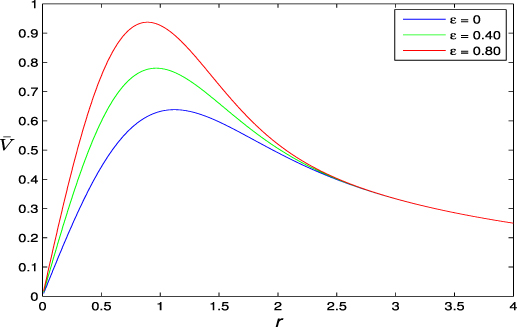
Figure 1. Velocity profiles for the perturbed Lamb–Oseen vortex as ε is varied.
Download figure:
Standard image High-resolution imageTo show that the perturbed vortex (2) is at least locally unstable it is convenient to first note that the Rayleigh discriminant can be expressed in terms of the angular velocity  and the axial vorticity ζ by writing
  . For the particular case of the velocity profile (2), we obtain

According to Sturm–Liouville theory, there will be instability, so long as Φ is negative for some value of r and we see from (3) that this condition can always be satisfied for the velocity profile (2). (For  will be negative only very far from the vortex center, so the instability will be extremely weak. Although instability is also possible for ε < 0, the corresponding growth rates were found to be small; we will therefore present results only for positive ε.)
Non-axisymmetric perturbations are also of interest in our study and for that case, a second theorem due to Rayleigh is pertinent. The latter theorem applies only if k = 0 and it provides a necessary condition for instability, namely, that  change sign at some value of r. For the velocity profile (2), we obtain as the necessary condition

for some value of r. Equation (4), unlike (3), is not a sufficient condition for instability and we will see that although this condition is satisfied in our case, it does not lead to instability..
Michalke and Timme (1967) have reported an investigation of unstable vortices whose spirit is similar to that of the present paper. However, the application of primary interest to these researchers was to the stability of spanwise vortices that appear downstream of the initial instability in a two-dimensional mixing layer. They considered both broken-line profiles and the continuous vortex with velocity profile

The profile (5) was chosen to reproduce features observed in mixing layer experiments. In particular, the vorticity is concentrated in a band more or less centered at r = 1, which is where the maximum occurs. The Rayleigh discriminant  for the above profile, so it is stable to axisymmetric perturbations. However, a sufficient condition for instability derived by Howard and Gupta (1962) suggests that instability is possible for helical perturbations with
  . Michalke and Timme showed that, in fact, such instabilities do occur for their profile with the largest growth rates obtained for k = 0. Since
  , the necessary condition for instability (4) is satisfied for the velocity profile (5). It is, nonetheless, surprising that the largest growth rates were obtained for k = 0. We will see in section 3 that this is not the case for our velocity profile (2); further comparisons will be deferred until that section.
Although there are no general stability criteria for non-axisymmetric perturbations, an approximate generalization of Rayleigh's sufficient condition for instability was derived by Billant and Gallaire (2005). Their development assumes that k is large and employs the WKB method in a manner similar to Le Dizès and Lacaze (2005). We will see in section 3 that predictions using their analysis agree well with our numerical results for the onset of instability for the first two helical modes even though assumptions in their analysis about the eigenfunction are not satisfied.
Finally, there are important applications in geophysical fluid dynamics, where the stability of vortices is pertinent. Gent and McWilliams (1986) made the point that vortices with velocity profiles behaving as potential vortices in the far field decay too slowly to accurately describe, for example, tornadoes. For that reason, they investigated several models with velocity profiles such as  that have zero total circulation in the far field. It will be seen in section 3 that although the far field velocity profile of a vortex does influence its stability, the most unstable modes of the perturbed Lamb–Oseen vortex do behave in a manner similar to those for the vortices considered by Gent and McWilliams.
2. Stability equation and analysis
Our objective, as stated above, is to investigate the instability of a vortex whose velocity components, in cylindrical coordinates, can be written ![$[0, \bar{V} (r), 0]$](https://content.cld.iop.org/journals/1873-7005/54/1/015513/revision3/fdrac522dieqn20.gif) . To that end, a helical perturbation of
. To that end, a helical perturbation of  is superimposed on the mean flow and we write for the radial, azimuthal and axial velocity, respectively,

The pressure

where  is the pressure of the unperturbed vortex. The axial wavenumber is denoted k, m is the azimuthal wavenumber and
  is the complex frequency. Substituting these expressions into the inviscid momentum equations, the continuity equation, and then linearizing, one can eliminate all variables but u to obtain the stability equation derived by Howard and Gupta (1962), namely,

where
 is the angular velocity of the mean flow,
  is its axial vorticity and
At this point, the numerical procedure to solve the eigenvalue problem will only be outlined, because it will be seen that the axisymmetric case requires a different method from that used to deal with the helical case  . A more detailed presentation will be given in section 3. In all cases, though, the range of integration is from r = 0 to
  . There is a regular singular point at r = 0, whereas the singularity at infinity is irregular. Series solutions will be employed to begin the integration at either end and the solutions matched at an interior point by requiring the Wronskian to vanish.
Near the origin, the solution can be represented by a Frobenius expansion having the form

so that the radial perturbation velocity vanishes at the center of the vortex except in the case  , the so called bending mode, and then it is continuous. The coefficient a2 of the r2 term is given by
where  and
and  .
.
Far from the center of the vortex, the velocity profile can be be approximated as a potential vortex so that  . Employing that approximation, it can be shown that w, the axial velocity perturbation, satisfies a modified Bessel equation and Km
is the solution that decays as
. Employing that approximation, it can be shown that w, the axial velocity perturbation, satisfies a modified Bessel equation and Km
is the solution that decays as  . From the linearized equations of motion,
  and using the asymptotic expansion for
  , we find that for large r

A derivation of the far field solution is given in Ash and Khorrami (1995), but their asymptotic solutions (8.2.130b) are incorrect because they are missing the square roots.
2.1. Theory for axisymmetric modes
Setting m = 0 greatly simplifies the Howard–Gupta equation (8) and if, in addition, we let  , the following Sturm–Liouville form results:

where  and
and  is the Rayleigh discriminant. The boundary conditions are homogeneous with
  near r = 0 and
  exponentially as
  . Before discussing the stability conditions with respect to the Rayleigh discriminant
  , we will prove the following necessary condition for instability involving the complex constant ω, whose imaginary part is the amplification factor.
Multiplying (11) by  and integrating between the boundaries, we obtain for the imaginary part of the resulting equation

where the homogeneous boundary conditions have been employed. Assuming that there is instability, i.e.  , (12) can be satisfied only if
  . We will see that this is true only for axisymmetric modes and is generally not the case for the helical modes.
Having established now that  for axisymmetric perturbations, we can see that if k is
  ,
,  will be a large negative number that becomes infinite as
  . It is therefore of interest to consider the product
  appearing in (11) and figure 2 below shows
  . Loosely speaking,
  must be positive for some range of r in order that the eigenfunction will be oscillatory there, thus permitting the homogeneous boundary conditions to be satisfied. We see in figure 2 that in the region where Φ is negative that its magnitude is small. It will not be surprising then to see in the results below that λ must be very large for instability of any magnitude to occur. The numerical consequences of this will now be discussed.

Figure 2. Variation of the Rayleigh discriminant with radius for the perturbed Lamb–Oseen vortex ![$\bar{V} = \left[1 - (1 - \varepsilon r^2 ) e^{- r^2}\right]/r$](https://content.cld.iop.org/journals/1873-7005/54/1/015513/revision3/fdrac522dieqn52.gif) .
.
Download figure:
Standard image High-resolution image2.2. Computational issues for axisymmetric modes
It will be seen below that the eigenfunctions grow very rapidly as we integrate outward from r = 0. That being the case, it is easier to solve the equation for u than to solve (11) for g, because near the center of the vortex  , whereas
  . The equation satisfied by u in the axisymmetric case m = 0 is the following:

Near the origin, it is obvious from (3) that the Taylor series expansion of Φ is of the form

It follows that to lowest order in r, u satisfies the modified Bessel equation. Only one solution is bounded at r = 0, namely,

For large values of its argument, I1 grows exponentially and that will be the case here because k is typically  and
and  . Only when r is very small does u grow linearly in r and the Frobenius series below can be used to initiate the integration.
Unlike (8), the governing equation for helical modes, there are no singular points in (13) apart from the boundaries, so a straightforward Runge–Kutta procedure can be used to carry out the integration. Taking account of the rapid growth of u discussed above, we can utilize a power series to begin the integration outward towards a value of r where a matching condition to the outer solution is imposed. For the example used to illustrate the situation, the integration was initiated at r = 0.01 and a small step size, again equal to 0.01 was employed. Near the vortex center, we find that the solution can be written

where
The asymptotic far field boundary condition for the outer solution can be obtained from equation (10) by simply setting m = 0. Given that  , it is sufficient to approximate u by the leading order term in (10). The second condition required to initiate the inward integration of (13) is obtained by differentiating the asymptotic form for u, which leads to

To solve the eigenvalue problem, we first integrate outward from r = 0.01 and then integrate inward from r = 6 to an interior matching point that can be chosen by trial and error. It is most convenient to fix ε and k while iterating on λ until the Wronskian of the two solutions vanishes at the chosen interior point. Either arbitrary constant can then be multiplied by an appropriate factor to arrive at an eigenfunction that is continuous.
The shooting method described above was usually successful for values of  . However, it was difficult to obtain a converged solution for larger values of
  . The eigenfunction in figure 3 below illustrates the difficulty, i.e. the rapid growth of u as we integrate away from r = 0. For this case,
  and the solvability condition of vanishing Wronskian was imposed at
  . A converged solution was obtained for
  , which corresponds to an amplification factor
  .
.

Figure 3. Eigenfunction for the axisymmetric mode with  and
and  .
.
Download figure:
Standard image High-resolution imageAs predicted by (15), the solution for u begins to grow exponentially not far from the vortex center. Moreover, the numerical solution shows that this extremely rapid growth continues even beyond r = 1. Clearly, our shooting method needs to be modified in order to find solutions when  is very large. Such a method will be described in the following section. We note, in passing, that similar problems were encountered by Smyth and McWilliams (1998) in their investigation of the linear instability of a vortex in the context of geophysical fluid dynamics. Specifically, they were unable to treat unstable modes, known to be present, when the density stratification was large compared to the planetary rotation.
3. Computational procedures and results
As suggested above, the numerical method employed in the axisymmetric case must be different from that used to deal with helical modes. The two principal differences are consequences of the result  when m = 0. At first sight, the helical case would appear to be more difficult, because an indented contour is required to deal with the critical point singularity and the eigenvalue iteration involves two constants (which we will choose to be
  and
and  ), rather than just
  . The greater challenge, however, is with the axisymmetric problem, owing to the magnitude of the eigenfunction u(r), as illustrated in figure 3. Even with the arbitrary constant
  , the eigenfunction u reaches a maximum value slightly larger than
  . A numerical method will now be presented that is able to treat this situation.
3.1. Numerical method and results for axisymmetric modes
It was pointed out below (15) that there is a region not far from the origin where u grows exponentially and an example was presented to illustrate the consequences of this growth. Given that  also grows exponentially at the same rate, we can define a new dependent variable proportional to
  that should be better behaved. This method, used previously to treat the stability of two-dimensional free shear layers (Michalke 1965, Maslowe and Kelly 1971), leads to a nonlinear first order equation and is known as a Riccati transformation. An apparent complication in the axisymmetric case, however, is that
  ; this can be seen from the Frobenius expansion (16). To remove the singularity at r = 0, we modify the usual transformation by writing

Substituting now the change of dependent variable defined by (18) into the governing equation for u, i.e. (13), leads to the Riccati equation

The procedure employed to solve the eigenvalue problem associated with (19) involves an inward and an outward integration, as before. Instead of requiring the Wronskian of the two solutions to vanish at the matching point, however, we now require that Q be continuous.
There are several possibilities to begin the outward integration, details of which can be deduced by first differentiating (18) and then introducing the Frobenius expansion (16) to approximate  . We obtain

where a2 and a4 are given below (16). In most cases, the outward integration was initiated at r = 0.02 with the initial value of Q provided by (20). Noting that  , (19) could also be linearized around r = 0 and the equation integrated. If Φ is expanded as in (14), then the first derivative at r = 0 is given by

and the integration could begin at r = 0. This, of course, is exactly the result obtained by differentiating (20) and setting r to zero.
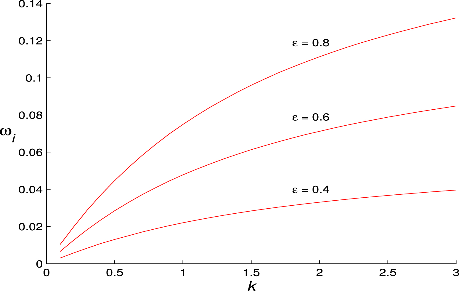
Figure 4 below presents the growth rates as a function of axial wavenumber for three different values of ε. We see that the instability is substantial and it increases monotonically with k in all cases. The qualitative behavior of ωi
as a function of k is similar to that reported by Billant and Gallaire (2005) for a family of zero circulation vortices relevant in geophysical applications with velocity profile  . Such behavior, termed 'ultraviolet catastrophy' in the vortex study of Smyth and McWilliams (1998), makes it clear that viscosity should be incorporated to obtain the correct behavior for short waves.

Figure 4. Variation of growth rate with axial wavenumber for the perturbed Lamb–Oseen vortex as ε is increased.
Download figure:
Standard image High-resolution imageTo obtain the results in figure 4, we had to deal with values of  as large as 2000. Before employing the Riccati method to investigate the stability of the perturbed Lamb–Oseen vortex, the program was tested on the case
  and the results seemed to agree well with those in figure 1(a) of Billant and Gallaire (2005). A Chebyshev collocation method was employed in the latter study. We do not know if the authors chose
  from Sturm–Liouville theory or if they determined it by iteration, because nothing is said in their paper about
  . It will be seen below that
  in the case of nonaxisymmetric modes, so the question of its behavior should not be ignored.
The Riccati method was also used by Michalke and Timme (1967) to investigate the stability of the velocity profile (5). Their computations, however, did not face the same challenges as those in the present paper, because the vortex described by (5) is stable to axisymmetric perturbations. As noted in the introduction, the focus of their paper was on unstable nonaxisymmetric disturbances, so comparisons will be deferred to the following sub-section.
3.2. Numerical method and results for helical modes
We present in this section results obtained by solving the Howard–Gupta equation (8) for non-axisymmetric perturbations with m = 1 or m = 2. It will be seen that the growth rates decrease rapidly with increasing m, so there is little point in considering values of m > 2. The numerical procedure used will essentially be the shooting method described above in section 2.2. However, u and ω are now complex, so that the integration contour must be indented to avoid the critical point singularity, where  (recall that
  ). The viscous critical layer analysis of Le Dizès (2004) shows that the correct eigenvalue condition for a neutral mode is obtained by considering the limit
  . For our vortex, this means that the integration contour must pass above the singularity, a consequence of
  being negative.
The stability calculations for the m = 1 mode are of particular interest for several reasons. This mode is distinctive because it is the only mode with nonzero radial velocity at the vortex center. That characteristic makes its presence clearly visible in the elliptical instability experiments of Leweke and Williamson (1998). Although most related studies indicate that other values of  lead to larger growth rates in the inviscid case, Mayer and Powell (1992) present some results for the Batchelor vortex suggesting that this may not be the case when viscosity is included.
In figure 5 below, results are presented for both the real and imaginary parts of ω as a function of ε with the wavenumber fixed at the value k = 1.50. We see from figure 5(a) that unlike the axisymmetric mode, the frequency ωr
is nonzero and it increases quite rapidly with ε. With regard to the amplification rates, at the chosen value of k, the bending mode is damped very slightly until ε reaches about 0.22. Although it increases rapidly beyond this value of  is still smaller than it is for the m = 0 case. For example, at
  for the bending mode compared with 0.0960 for the axisymmetric disturbance. Given that the wavenumber corresponding to the largest amplification rate increases very slowly with ε, figure 5(b) depicts quite closely the maximum value of
  as a function of ε.

Figure 5. Variation of the complex frequency for the bending mode m = 1 as ε is varied with a constant axial wavenumber k = 1.50.
Download figure:
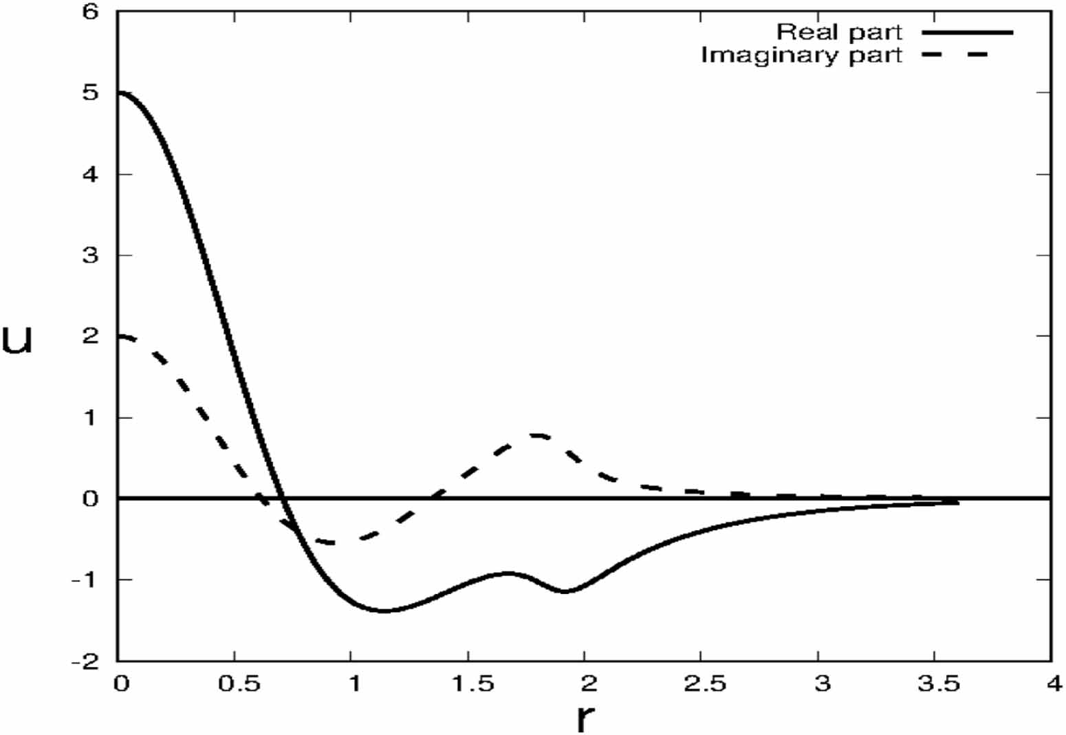
Standard image High-resolution imageContinuing now with the behavior of the bending mode, we examine the eigenfunctions and show that they do not resemble those of the axisymmetric case. They are, of course, complex and are nonzero at the vortex center. In addition, they oscillate slightly, particularly for  values of r. Although the author has examined eigenfunctions for many different axial wavenumbers and even some for higher modes, the one illustrated in figure 6 is sufficient to exhibit these differences compared with the axisymmetric mode shown in figure 3. The magnitude of
  is directly related to the term
  , which multiplies
  in (8). This term is much smaller in the case of the bending mode, as a direct result of the fact that m and
  are nonzero when
  . In the axisymmetric case,
  becomes equal to
  , which is very large when k is large and/or
  is small.

Figure 6. Typical eigenfunction for the m = 1 bending mode. The mean flow profile is that of a perturbed Lamb–Oseen vortex;  and
and  .
.
Download figure:
Standard image High-resolution imageTo conclude our presentation of results on the stability of the perturbed Lamb–Oseen vortex to helical perturbations, we compare growth rates for the m = 2 mode with those of the bending mode m = 1. Figure 7 presents a comparison of amplification rates for these two modes at a value of ε = 0.6. It is, perhaps, surprising that the amplification rate of the m = 2 mode is so much smaller. However, this is consistent with results in figure 1(a) of Billant and Gallaire (2005) for the vortex  . A qualitative difference that should be pointed out, however, is that both stability curves in figure 7 contain a value of k where the growth rate is maximum. This is, of course, normally the case, but it is not true for the vortex
  where ωi
continues its monotonic growth with k. A related point of some interest is the behavior of these stability curves at what we can term the critical values of k. As k increases near 1.04, the m = 1 mode goes from being damped to becoming amplified. Near the other end, however, the stability curve never intersects the k-axis and this mode becomes a Kelvin wave. The same behavior is observed for the m = 2 helical mode.
where ωi
continues its monotonic growth with k. A related point of some interest is the behavior of these stability curves at what we can term the critical values of k. As k increases near 1.04, the m = 1 mode goes from being damped to becoming amplified. Near the other end, however, the stability curve never intersects the k-axis and this mode becomes a Kelvin wave. The same behavior is observed for the m = 2 helical mode.
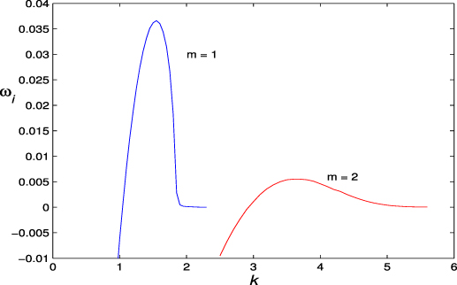
Figure 7. Stability diagram for the helical modes with azimuthal wavenumbers m = 1 and m = 2. The azimuthal velocity profile is the perturbed Lamb–Oseen vortex with ε = 0.6.
Download figure:
Standard image High-resolution imageFinally, we compare the results obtained in this section with those of Michalke and Timme (1967), who investigated the velocity profile (5). As noted in the Introduction, this velocity profile is stable to axisymmetric perturbations. However, the possibility of instability to non-axisymmetric perturbations is suggested by (21) of Howard and Gupta (1962). In the absence of axial flow, the latter result can be written

is a sufficient condition for stability. Clearly, for helical modes there will always be a value of k small enough that this condition is violated. That does not guarantee instability, however, and computations must be carried out for specific cases to see if and when instability occurs. That said, let us now briefly summarize the results presented by Michalke and Timme for the continuous profile (5).
First of all, the behavior of  with k is the exact opposite of that found for either the perturbed Lamb–Oseen vortex or the profile
  . The largest growth rates were obtained at k = 0 and ωi
was found to decrease rapidly with increasing k. Secondly, the azimuthal wavenumber leading to the largest growth rates was m = 4; for m = 3 and m = 5, the maximum value of
. The largest growth rates were obtained at k = 0 and ωi
was found to decrease rapidly with increasing k. Secondly, the azimuthal wavenumber leading to the largest growth rates was m = 4; for m = 3 and m = 5, the maximum value of  was approximately 25% smaller and for m = 1 only a neutral mode was found. Possibly, these results are related to the behavior near r = 0 of the model employed in Michalke and Timme (1967), i.e.
  , as opposed to the rigid rotation characteristic of most vortices. (We note, in passing, that the ordinate of figure 4 in their paper is labeled incorrectly. This figure shows the growth rate for a discontinuous model, so it is not directly related to this paper.)
3.3. Extension of Rayleigh's criterion to helical modes
As cited in the Introduction, an approximate generalization of Rayleigh's criterion for axisymmetric disturbances was derived by Billant and Gallaire (2005). Their development assumes that k is large and the WKB method was utilized. The eigenfunction in their analysis was assumed to have two turning points, implying an oscillatory region along the real axis between the Stokes lines emanating from these turning points. Outside of the oscillatory region, the eigenfunction was represented by the usual exponentially growing and decaying WKB functions. In the large k limit, it was ascertained by Billant and Gallaire (2005) that the onset of instability is determined by first finding the value  , where
  The desired value of r0 is obtained by solving the implicit equation

A generalized Newton iteration was used to solve (23) for r0 and it was found to converge rapidly even when the initial guess was inaccurate. Once r0 has been obtained, ω, the complex frequency, is given by the equation

Some results for azimuthal wavenumbers m = 1 and m = 2 are presented in table 1. We see that the onset of instability is predicted by (24) to occur at ε ≈ 0.22 for the m = 1 bending mode and ε ≈ 0.51 for the m = 2 helical mode. Using the method described in section 3.2, the actual computed results for the critical values of ε were found to be 0.21 for m = 1 and ε = 0.52 for m = 2. In both cases, the predictions based on large-k asymptotics are seen to be remarkably accurate. This is less surprising in the m = 2 case, because the corresponding value of k is 3.28 and the expansion is in powers of k−2. However, for m = 1 the wavenumber at the stability boundary was k = 1.5, so the method seems to work well even for waves that are not extremely short. The eigenfunctions (see e.g. figure 6) computed by the author do not resemble the configuration assumed by Billant and Gallaire, so we must conclude that their method does not require a faithful representation for u(r) in order to yield accurate predictions for the onset of instability.
Table 1. Frequency and amplification factors for helical modes m = 1 and m = 2 near the critical values of ε.
| m | ε | r0 | ωr | ωi |
|---|---|---|---|---|
| 1 | 0.20 |
| 0.1633 | −0.000035 |
| 1 | 0.22 |
| 0.1745 |

|
| 1 | 0.24 |
| 0.1836 | 0.00101 |
| 2 | 0.50 |
| 0.6338 |

|
| 2 | 0.51 |
| 0.6402 |

|
| 2 | 0.52 |
| 0.6468 | 0.00036 |
| 2 | 0.54 |
| 0.6598 | 0.0016 |
4. Concluding remarks
In the introduction of this paper, it was pointed out that despite an extensive literature dealing with the stability of vortices, very few articles investigate the instability of a single vortex with no axial flow. Most studies of wave-like perturbations on vortices have instead concerned the propagation of Kelvin modes. An example is the discontinuous Rankine vortex comprised of an inner region of rigid rotation and an outer region, where the behavior is that of a potential vortex  . In the case of the more realistic Lamb–Oseen vortex, some new modes exist owing to the presence of a critical layer. However, these modes turn out to be damped, which is disappointing from the standpoint of hydrodynamic stability theory.
It appears that the paper by Michalke and Timme (1967) was the first to actually investigate numerically the instability of a continuous, unbounded vortex. As discussed in section 3.2, the approach of Michalke and Timme was somewhat different from our own in that their goal was to demonstrate that a vortex, stable according to Rayleigh's circulation theorem, could be destabilized by a non-axisymmetric disturbance. As an example of a continuous model, they showed that the vortex with velocity profile (5) was unstable to helical perturbations having azimuthal wavenumbers  . In addition to being of interest in its own right, this result shows that the analysis in section 4 of Billant and Gallaire (2005) is sometimes incorrect. The latter purported to demonstrate that axisymmetric modes always have higher growth rates than helical perturbations, which is clearly not the case for the vortex profile (5).
In this paper, the author has shown that a slight perturbation of the stable Lamb–Oseen vortex can give rise to instabilities of significant growth rate. The results presented in sections 3.1 and 3.2 show that the growth rate  of these disturbances becomes large when
  the perturbation parameter, is increased beyond infinitesimal values. This is particularly true for axisymmetric modes as k, the axial wavenumber, becomes large. The monotonic increase in growth rate with k shown in figure 4 was previously observed in the case of the velocity profile
  , as reported by Billant and Gallaire (2005). For the helical modes of azimuthal wavenumber m = 1 and m = 2, on the other hand, ωi
behaves in a more conventional way in the case of the perturbed Lamb–Oseen vortex. As shown in figure 7, there is a finite range of unstable wavenumbers, whereas the growth of
, as reported by Billant and Gallaire (2005). For the helical modes of azimuthal wavenumber m = 1 and m = 2, on the other hand, ωi
behaves in a more conventional way in the case of the perturbed Lamb–Oseen vortex. As shown in figure 7, there is a finite range of unstable wavenumbers, whereas the growth of  continues to be monotonic with increasing k for the vortex
  .
.
Even though the hydrodynamic stability characteristics of a single vortex are known for only a few cases, we can still make some general observations on what has been learned up to this point. First of all, the largest growth rates are usually associated with axisymmetric modes, where there is a monotonic increase of  with k in all cases of a vortex whose angular velocity is nonzero at its center. This suggests that centrifugal instability is the dominant mechanism, as opposed to shear instability. That being the case, one can assume that the velocity of the vortex at the value of r where Φ changes sign is related to the growth rate. For the perturbed Lamb–Oseen vortex, equation (3) shows that Φ, the Rayleigh discriminant, becomes negative for
  . As ε increases from zero,
  moves in from infinity,
  increases and so does the amplification factor of the instability, as shown in figure 4.
The occurrence of a maximum growth rate as  is associated with centrifugal instability and contrasts totally with the behavior of the non-axisymmetric modes for the vortices investigated by Michalke and Timme (1967). The latter authors studied three vortex models, two of which had discontinuous vorticity profiles, and in all 3 cases the largest growth rates were obtained for k = 0. This behavior suggests a shear layer mode of instability. The one instance where similar behavior was observed in Billant and Gallaire (2005) was for the case of a vortex with velocity profile
  , where the growth rate was nonzero at k = 0 when m = 2 and m = 3. The monotonic growth of ωi
with k was found, however, to still occur as
, where the growth rate was nonzero at k = 0 when m = 2 and m = 3. The monotonic growth of ωi
with k was found, however, to still occur as  .
.
From the results obtained to date, it is obvious that numerical solution of the Howard–Gupta equation (8) is required to determine the stability properties of a single vortex having a continuous velocity profile. Even in cases where the Rayleigh criterion guaranties instability one does not know the value of the axial wavenumber k corresponding to the onset of the instability. As for the value of k yielding the maximum growth rate, the examples reviewed above reveal that any value is possible, including k = 0. The results presented in figures 4–7 of this paper suggest a number of potentially interesting extensions. The most obvious would be to see if the addition of a slight viscosity would damp the short-wave instability evident in the axisymmetric mode shown in figure 4. Other effects whose incorporation would be of interest could include density stratification and/or nonlinearity.
Finally, there are important applications in geophysical fluid dynamics, such as tornadoes, that were mentioned briefly in this paper. Gent and McWilliams (1986) argued that vortices with velocity profiles behaving as potential vortices in the far field decay too slowly to accurately simulate these phenomena. Instead, they investigated several models with velocity profiles such as  that have zero total circulation. Given that computational issues limited the extent of the results reported in both Gent and McWilliams (1986) and Smyth and McWilliams (1998), it would be interesting to expand those results using a more robust scheme; for example, the Riccati method described in section 3.1.
Acknowledgments
The author is pleased to acknowledge the assistance of several colleagues in the preparation of this article. These include Peter Bartello, David Jeffrey, Bruce Yin and Gantumur Tsogtgerel.
Appendix.: Validation of numerical methods
There are many factors, in addition to integration step size, that influence the accuracy of computations of the sort presented above. At the suggestion of a referee, this appendix has been added to the paper in order to summarize the tests made to verify our results. We begin by a comparison with a result for a damped  mode on a Lamb–Oseen vortex reported by Fabre et al (2006). Table 1 of their paper is intended to illustrate how, as the Reynolds number Re is increased, the solution tends towards the inviscid value given in the table caption as
  . Using the indented contour method described in section 3.2, the author obtains
  . Given the perfect agreement for the frequency
  , it was surprising to note the significant disagreement for
  . Fortunately, the values provided in table 1 of Fabre et al for Re
 and 105 make it clear that there is a typographical error in their inviscid result for
  . In other words, once that error is corrected, there is actually perfect agreement to five significant figures.
A similar comparison involving a non-axisymmetric m = 2 mode was not entirely possible because only results for Re were provided by Fabre et al (2006). It was nonetheless interesting to compare an inviscid computation with their result in figure 21(d) for k = 5, where it was found that
  . This compares with our inviscid result
  . The same tendencies are present as in the case of the bending mode with a somewhat greater damping effect of viscosity. This is due to the axial wavenumber k = 5 being much greater than k = 1, as viscosity has a greater effect on short waves.
Our final comparison will be with results reported by Smyth and McWilliams (1998) and Billant and Gallaire (2005) for the vortex with velocity profile  . Given that the aforementioned papers contain figures, but no tabular results, the comparison must be qualitative. As shown in figure A1, the monotonic growth of ωi
with k for large values of k is similar to that illustrated in figure 1(a) of Billant and Gallaire (2005) and figure 4 of Smyth and McWilliams (1998). And, we recall that figure 4 of this paper for the case of the perturbed Lamb–Oseen vortex displays the same behavior.
. Given that the aforementioned papers contain figures, but no tabular results, the comparison must be qualitative. As shown in figure A1, the monotonic growth of ωi
with k for large values of k is similar to that illustrated in figure 1(a) of Billant and Gallaire (2005) and figure 4 of Smyth and McWilliams (1998). And, we recall that figure 4 of this paper for the case of the perturbed Lamb–Oseen vortex displays the same behavior.

Figure A1. Variation of growth rate with axial wavenumber for the vortex with velocity profile  .
.
Download figure:
Standard image High-resolution image
The computations shown in figure A1 were carried out using the Riccati transformation presented in section 3.1. For a number of values of k, the governing eigenvalue problem was also solved using the conventional shooting method described in section 2.2. Comparing the values for  to 4 significant figures, it was found that the discrepancy was never greater than 0.0001. Taking k = 1.5, for example, the Riccati method yielded
  compared with
  when solving equation (13), the second order ODE.
The factors varied to test the accuracy of our computations included integration step size, starting point of the integration in either direction, number of terms in the Frobenius solution and upper bound of the Wronskian at the value of r where the solutions were matched. The integrations were carried out in double precision and the results turned out to be surprisingly insensitive to all of these factors. As an example, the step size was varied with k = 3 when integrating equation (13) outward, again with the velocity profile  . The integration was normally initiated at r = 0.01 which was also the step size. As a test, the integration was initiated at r = 0.02 with a step size of
  and the solutions matched at r = 0.86. The Wronskian at the matching point was required to be less than 10−3 and the two solutions for
  turned out to be identical to five significant figures!