

Abstract
More than half of the world's population now lives in urban areas, and trends in rural-to-urban migration are expected to continue through the end of the century. Although cities create efficiencies that drive innovation and economic growth, they also alter the local surface energy balance, resulting in urban temperatures that can differ dramatically from surrounding areas. Here we introduce a global 1 km resolution data set of seasonal and diurnal anomalies in urban surface temperatures relative to their rural surroundings. We then use satellite-observable parameters in a simple model informed by the surface energy balance to understand the dominant drivers of present urban heating, the heat-related impacts of projected future urbanization, and the potential for policies to mitigate those damages. At present, urban populations live in areas with daytime surface summer temperatures that are 3.21 ∘C (−3.97, 9.24, 5th–95th percentiles) warmer than surrounding rural areas. If the structure of cities remains largely unchanged, city growth is projected to result in additional daytime summer surface temperature heat anomalies of 0.19 ∘C (−0.01, 0.47) in 2100—in addition to warming due to climate change. This is projected to raise the urban population living under extreme surface temperatures by approximately 20% compared to current distributions. However we also find a significant potential for mitigation: 82% of all urban areas have below average vegetation and/or surface albedo. Optimizing these would reduce urban daytime summer surface temperatures for the affected populations by an average of −0.81 ∘C (−2.55, −0.05).
Export citation and abstract BibTeX RIS

Original content from this work may be used under the terms of the Creative Commons Attribution 4.0 license. Any further distribution of this work must maintain attribution to the author(s) and the title of the work, journal citation and DOI.
1. Introduction
More humans now live in cities than in rural areas, and urbanization is expected to intensify over the next century (Grimm et al 2008). The concentration and density of humans in urban settlements has driven innovation and economic growth by simultaneously increasing the efficiency of human transactions and interactions, and by providing returns to scale on infrastructure investments (Hanson 2001, 2005, Bettencourt et al 2007, Bettencourt 2013). However, conversion of natural landscapes to urban ones has also dramatically changed the urban energy balance, resulting in different, often higher, local temperatures experienced by inhabitants. This so-called urban heat island (UHI) effect has important potential consequences for city populations: atmospheric UHIs increase vulnerability to heat-related morbidity and mortality (Patz et al 2005, Luber and McGeehin 2008, Mora et al 2017) and affect the energy demand and efficiency of the urban population through altered heating and cooling needs (Santamouris 2014b).
Urban heat anomalies are usually quantified as UHI Intensities—the difference between the temperature (atmospheric, surface, or groundwater) of a city as a whole and its surrounding rural background (Howard 1818, Oke 1973, Kalnay and Cai 2003); recent studies have begun to assess the global variability of surface UHI Intensities (Peng et al 2011, Chakraborty and Lee 2019) and the relationship of urban heat with factors like city size (Huang et al 2019, Manoli et al 2019) and climate (Scott et al 2018). However, this city-level metric is inadequate for characterizing the consequences of urban temperature anomalies at higher spatial resolution. Indeed, a number of localized studies have shown that within-city variations in urban temperatures can be large (Grimmond 2007), and larger-scale efforts have classified UHIs of selected cities into local climate zones to account for heterogeneity in the urban morphology and landscape characteristics (Stewart and Oke 2012, Yang et al 2021). Yet to date, a comprehensive assessment of drivers and impacts of urban temperature anomalies both within individual cities and at global scale has been lacking.
Here we introduce a global assessment of local (1 km) surface temperature anomalies (ΔT). We derive the average ΔT—total, seasonal, and diurnal—for the world over the past decade to quantify the heat burden created by the current distribution of human population and city structure. We then use a simple empirical model informed by the surface energy balance (Oke 1988) to test the physically-predicted relationships between local surface temperature anomalies and a set of observable and scalable measures on a global scale. We combine these relationships with a set of potential urbanization futures to derive likely distributions of urban surface temperatures at the end of the century, and discuss their impact on the number of people living under extreme temperatures.
2. Global patterns of urban surface temperature anomalies
We define ΔT for each 1 km pixel, i, as the difference between local satellite-observed land surface temperature (LST) and the median LST of rural surrounding areas (Benz et al 2017):

LSTs are 10-year mean (2004–2014) seasonal daytime and nighttime surface temperatures from MODIS (Z Wan 2015a, 2015b). (See supplement S1 (available online at stacks.iop.org/ERL/16/064093/mmedia) for more information on data used in this study. LST images have an error  2 K—this error is not displayed in our analysis). Rural background pixels for comparison are defined as those falling within a 100 km distance of pixel i, with nighttime lights below a defined threshold, and similar elevation and aspect (see supplement 2.1). Figure 1(A) shows aggregated global patterns of urban ΔT; our accompanying app (https://sabenz.users.earthengine.app/view/surface-delta-t) shows full coverage and resolution. Although we calculate ΔT for all land areas, urban or rural, between −60∘ and 70∘ latitude, we highlight here a subset of 874 096 pixels (hereafter, urban pixels) defined by the Global Human Settlement Urban Center Database (Florczyk et al
2019). These urban agglomerations, defined by UN's Degree of Urbanization methodology, house a total of 2.288 billion people worldwide (hereafter, urban population). Figure 1(B) shows LST anomalies at full resolution, along with several defined urban agglomerations; our ΔT algorithm is sensitive enough to detect smaller urban settlements outside of the major urban areas defined by the GHS Database.
2 K—this error is not displayed in our analysis). Rural background pixels for comparison are defined as those falling within a 100 km distance of pixel i, with nighttime lights below a defined threshold, and similar elevation and aspect (see supplement 2.1). Figure 1(A) shows aggregated global patterns of urban ΔT; our accompanying app (https://sabenz.users.earthengine.app/view/surface-delta-t) shows full coverage and resolution. Although we calculate ΔT for all land areas, urban or rural, between −60∘ and 70∘ latitude, we highlight here a subset of 874 096 pixels (hereafter, urban pixels) defined by the Global Human Settlement Urban Center Database (Florczyk et al
2019). These urban agglomerations, defined by UN's Degree of Urbanization methodology, house a total of 2.288 billion people worldwide (hereafter, urban population). Figure 1(B) shows LST anomalies at full resolution, along with several defined urban agglomerations; our ΔT algorithm is sensitive enough to detect smaller urban settlements outside of the major urban areas defined by the GHS Database.
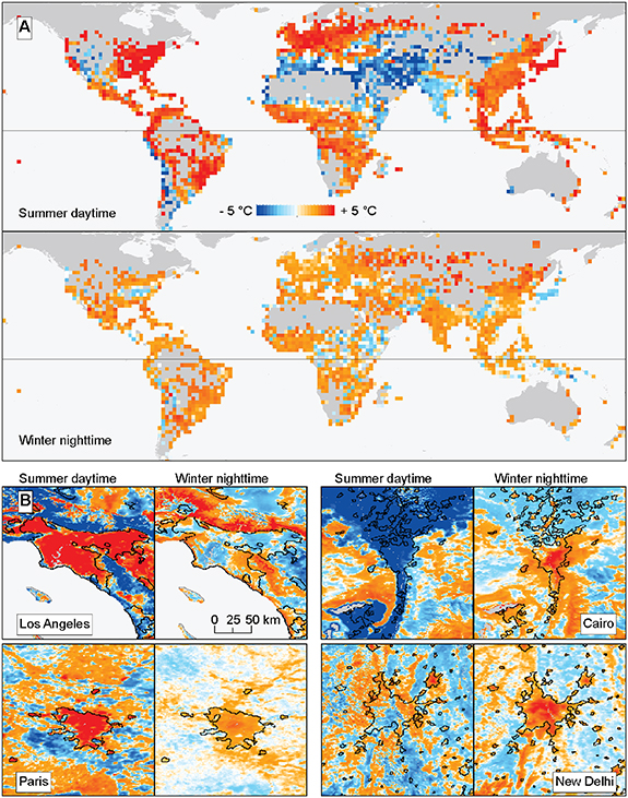
Figure 1. (A) Map of urban surface temperature anomalies (ΔT). Shown is the average of all urban pixels in each grid cell (aggregated to a 2∘ grid to show basic distribution). (Full 1 km resolution data are available at https://sabenz.users.earthengine.app/view/surface-delta-t). Grid cells not included in a city defined by the Urban Center Database (Florczyk et al 2019) are left blank. (See figure S1 for all seasons and annual mean). (B) Summer daytime ΔT and winter nighttime ΔT for selected locations. Shown are urban and non-urban ΔT, outlines of cities are shown in black.
Download figure:
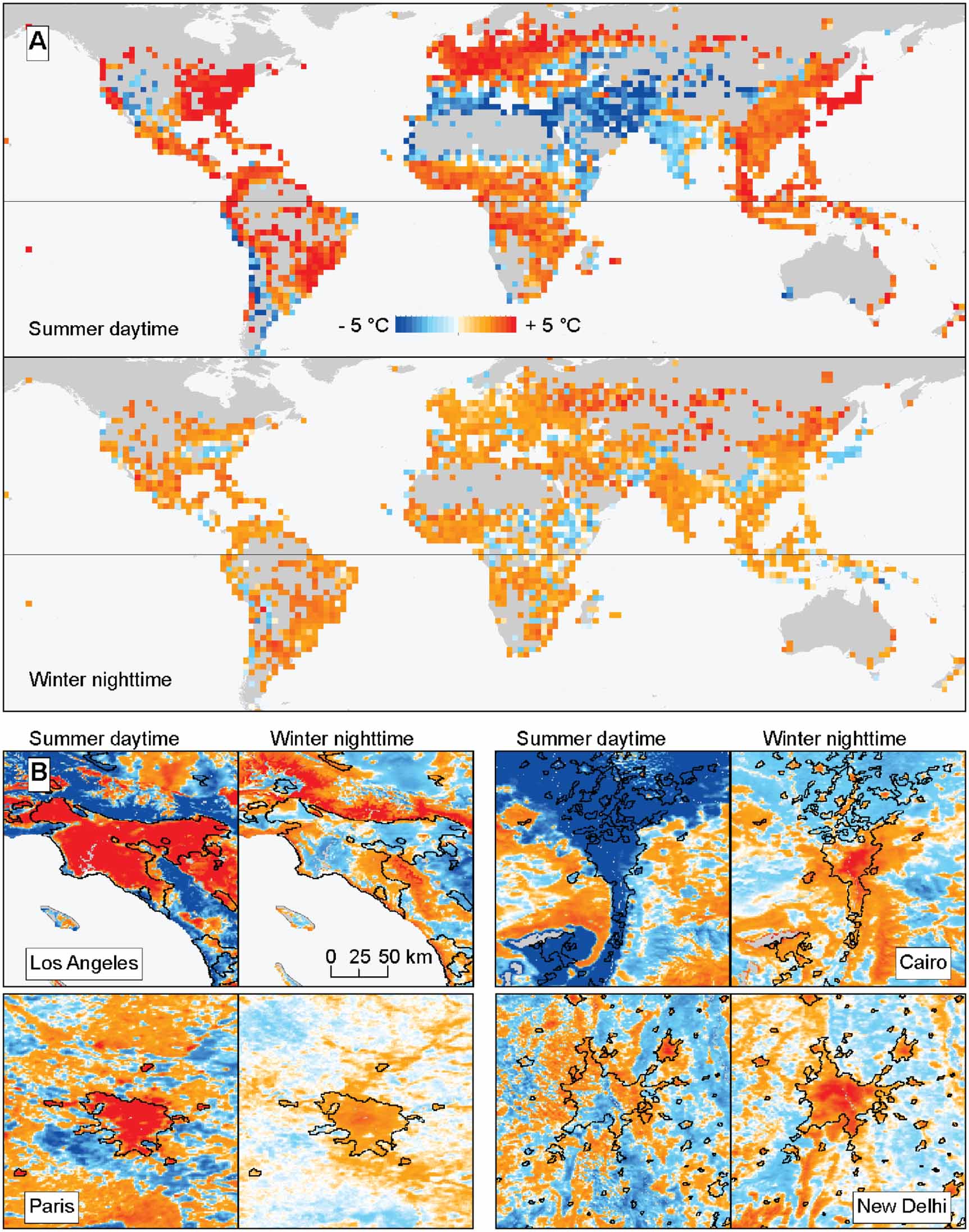
Standard image High-resolution imageWe find that 67% of all urban pixels (housing 75% of the urban population) show daytime and nighttime warming (upper right quadrants in figure 2(A)), while 9% of urban pixels (5% of urban population) show warming only during daytime, and 19% (17% of urban population) show warming only at night. Globally, on average, each person living in an urban area is exposed to annual mean surface temperature anomalies of +2.11 ∘C (−2.58, 7.10, 5th–95th percentiles) during daytime (+3.21 ∘C (−3.97, 9.24) in Summer and +0.94 ∘C (−2.27, 5.24) in Winter) and +1.49 ∘C (−0.20, 3.91) during nighttime (+1.70 ∘C (−0.18, 4.59) in Summer and +1.34 ∘C (−0.75, 4.76) in Winter). Presently, 55% of the urban population lives in areas with average summer daytime surface temperatures greater than 35 ∘C, compared to 33% of people in rural areas. If cities did not create these surface temperature anomalies, only 23% of the urban population would live under such extreme daytime summer surface temperatures (figure 2(B)). Importantly, this pixel-scale analysis reveals a much higher population share in areas with extreme surface summer daytime temperatures: city-scale analysis underestimates the population living in areas with summer daytime temperatures above 35 ∘C by 13% and for areas above 38 ∘C by 36% (figure 2(B)).

Figure 2. (A) Heat map of daytime and nighttime urban surface temperature anomalies (ΔT) averaged over the whole year, and broken out by season (see figure S2 for spring and fall). Black markings indicate the mean point and 90% confidence ellipse. The total area and population represented in each quadrant is shown. (B) Distributions of average summer daytime (left) and average winter nighttime (right) surface temperatures that populations in cities are exposed to, compared to all other areas. In red the distribution based on average city surface temperatures. The light blue line shows the surface temperatures at the homes of the urban population in a scenario without urban heat (LST—ΔT). C: Heat map of the standard deviation (Std) of ΔT of each city within the Urban Center Database of the Global Human Settlement Layer (Florczyk et al 2019).
Download figure:
Standard image High-resolution imageWorldwide urban daytime ΔT tends to be more extreme than urban nighttime anomalies, with an average of 1.46 ∘C (−2.63, 5.83) compared to 1.00 ∘C (−0.48, 3.02). Similarly, urban summer ΔT is most extreme (daytime 2.14 ∘C (−3.97, 8.05) and nighttime 1.21 ∘C (−0.43, 4.03)). However, urban winter ΔT shows an increased range for nighttime (0.79 ∘C (−1.00, 3.49)) and a decreased range for daytime (0.79 ∘C (−2.07, 4.21)). For all seasons, the highest urban daytime surface temperature anomalies are found in Japan, and Central and South America. Urban cooling is primarily observed in dry areas of central Asia, North Africa, and the Middle East (figure 1(A)). Figures 1(B) and (S)3 show full resolution images of several archetypal locations. Although substantially different in climate and absolute surface temperatures, Parts of Los Angeles, California, US and Paris, France have summer daytime ΔT of more than 5 ∘C, and reduced nighttime warming (with slight cooling in LA). Cairo, Egypt and New Delhi, India are prime examples of urban cooling. Daytime summer LSTs in these cities are up to −5 ∘C lower than their background and ΔT becomes significant only at night within the city centers.
Our data reveal large within-city variance in surface temperature anomalies. We calculate a global average standard deviation of ΔT within each city to be 0.63 ∘C (0.12, 1.62) for daytime and 0.34 ∘C (0.06, 0.85) for nighttime (figure 2(C)). Broken out by season, within-city daytime standard deviation in ΔT increases in summer to 0.84 ∘C (0.17, 2.16), indicating the importance of analysis at local scales. We furthermore find qualitative evidence of the differential impacts towards different communities, with disadvantaged neighborhoods experiencing higher urban surface heat anomalies (figure S4) supporting claims by Chakraborty et al (2019) and Benz and Burney (2021).
3. Urban surface temperature anomalies and the surface energy balance
While a rich literature of localized studies has explored the relative importance of different energy fluxes and urban microclimate on temperature anomalies in very specific contexts, most large scale studies of urban heating have focused on empirical statistical relationships between temperature anomalies and simple metrics of city size, like population or area (Oke 1973, Zhou et al 2017, Huang et al 2019, Manoli et al 2019). This approach, however, conflates population density (the presence of more humans) with other structural qualities of cities that strongly govern the surface energy balance (Oke 1988, Grimmond et al 2010, Ward et al 2016, Fuladlu et al 2018) such as building density and height. Here we try to strike a balance between these two approaches: we construct an empirical statistical model informed by the urban surface energy balance and test whether these relationships hold globally at the pixel scale. To do this we relate our observed urban surface temperature anomalies (ΔT) to observable satellite-derived proxies for the relevant energy fluxes (see supplement S2.2 for derivation):

Here AHF is the anthropogenic heat flux, representing the heat output of humans both directly and through heating systems and electricity use. We use pixel-level population density (Pop) as a proxy for AHF. RR is reflected short-wave radiation shown as the difference between urban pixels u and their rural background r. Within cities, reflected radiation causes warming by being re-reflected and effectively 'trapped' by buildings in urban street canyons; we therefore use the normalized difference built-up index (NDBI) as a proxy for RR, calculating its anomaly analogously to ΔT as the difference between each pixel's value and its local median background value (a positive NDBI anomaly indicates more short-wave trapping in urban areas and less RR). Net heat storage (NHS) is driven by building materials in cities that can store heat. We find this effect reflected by satellite-derived black-sky albedo (BSA), since darker materials absorb incoming radiation (again we calculate the difference compared to rural background pixels). The sensible heat flux (SH) is determined by building materials and surface roughness, and thus proxied by both NDBI and albedo. Finally, LH, or latent heat flux, is driven by evapotranspiration, and we use the normalized difference vegetation index (NDVI) anomaly as a proxy (again, compared to background levels). These four proxies are not fully independent (e.g. NDVI/tree cover also affects reflected radiation), and they do not comprehensively describe all relevant city features (e.g. aerodynamic and moisture effects), but they are nevertheless useful for understanding the extent to which physical fluxes are represented by observable parameters at scale.
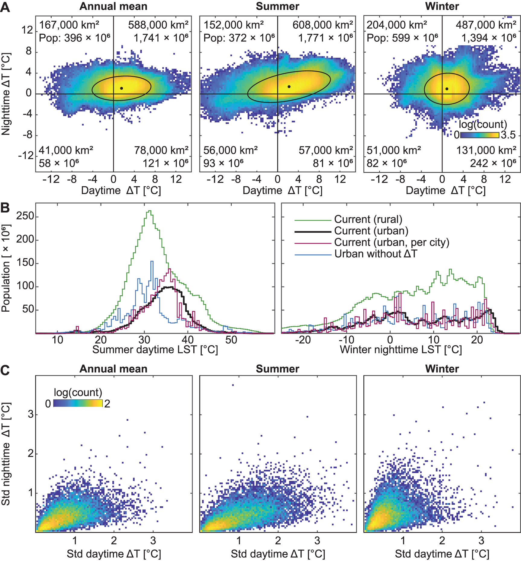
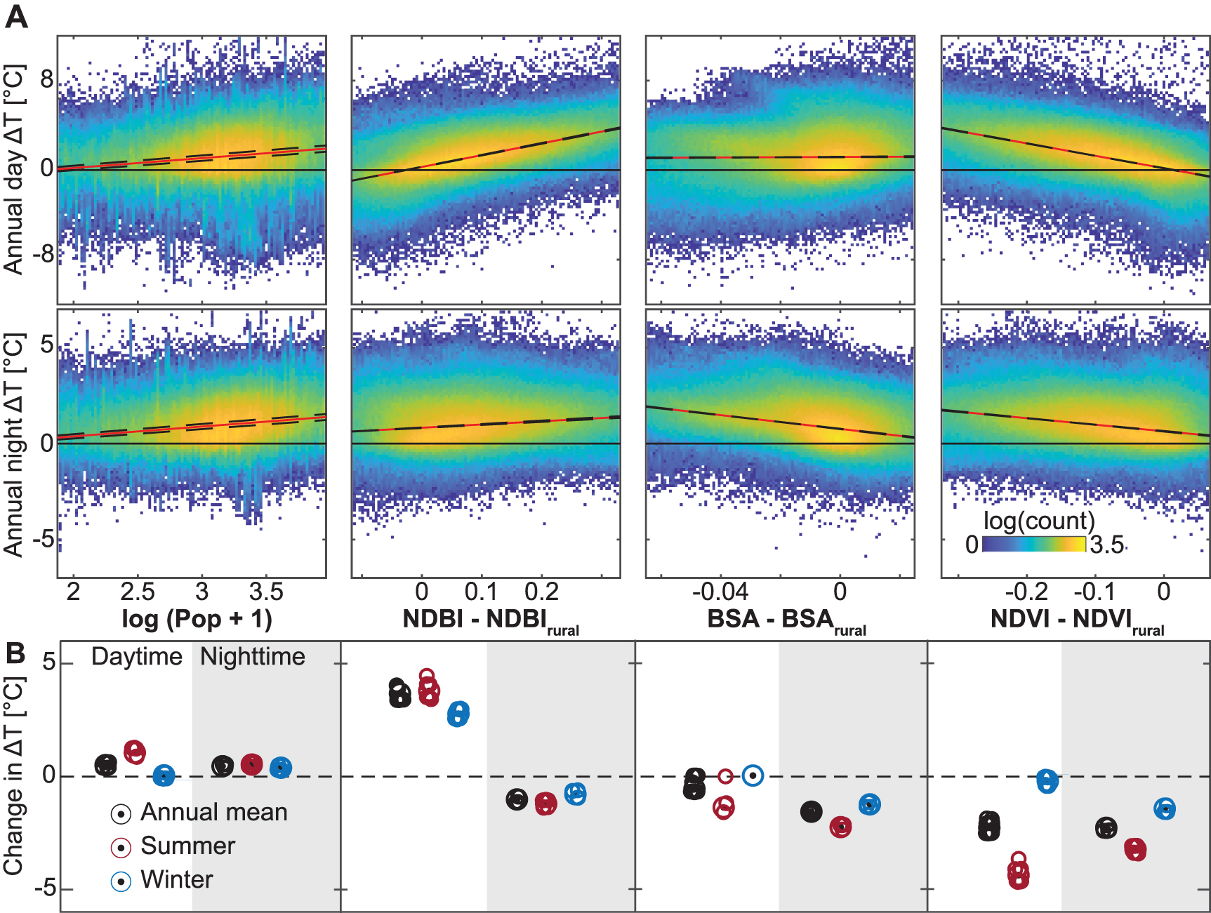
Indeed we find that urban ΔT is correlated with each of the four observed measures as expected from physical principles (figure 3(A)): ΔT is positively correlated with population density and NDBI anomaly, for both daytime and nighttime; since incoming radiation is much higher during daytime, the NDBI relationship is less pronounced at night, for population density the diurnal effect is much less pronounced but still significant (table S2). ΔT is inversely correlated with albedo—a low albedo anomaly means high positive NHS at daytime and negative at nighttime. In this global study, this effect is visible at night when stored heat is released. This contradicts previous findings for cities in the southern United States where a increase in albedo is linked to daytime cooling and has no effect at night (Zhao et al 2014). We understand this to imply that local conditions may vary. And finally, ΔT is inversely proportional to the NDVI anomaly, for both daytime and nighttime, with a stronger effect during the day. If NDVI within the city is higher than outside, which is commonly the case in more arid regions where vegetation within cities is irrigated, urban cooling is observed (e.g. figure 1(B)). These relationships also follow predicted patterns by season (figure S5) and when conducted as the average of each city included in the Urban Center Database (figure S6). It is also consistent with findings from figure 2(A)—pixels that show daytime and nighttime warming have high population density and NDBI but low NDVI whereas pixels with daytime and nighttime cooling are opposite (figure S7). Because we calculate ΔT and its drivers at the pixel level, we do not account for horizontal thermal or radiation exchange between neighboring pixels. We do observe a slight increase in average ΔT for cities of a larger size S8, consistent with observations of the impact of urban form on surface UHIs (Zhou et al 2017).
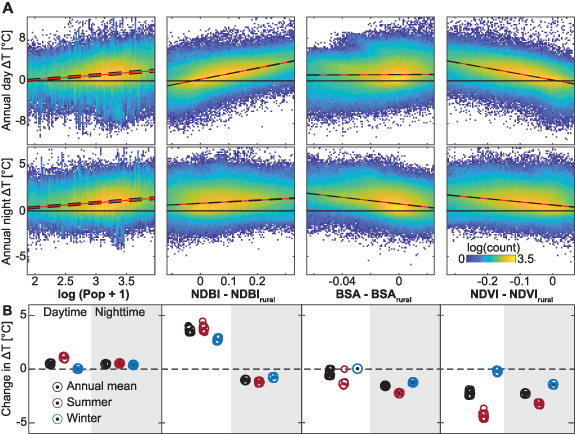
Figure 3. (A) Bivariate relationships between urban surface temperature anomalies (ΔT) and observable satellite measures impacting the surface energy balance. The inner 90 percentile of each parameter is fit with a simple linear regression, shown in red, 90% confidence interval are dashed in black (see table S2 for coefficients and goodness of fit; figure S5 for results of seasonal (summer and winter) ΔT). (B) Predicted changes in urban ΔT for each satellite measure, based on a multiple regression model including all four parameters. Shown is the predicted change in ΔT for a change in the predictor variable over the entire analyzed range (5th to 95th percentile). Uncertainties are constructed by conducting 1000 versions of the regression using sub-samples of data (see supplement S2.3); median regression is shown as a dot, outliers (following the box-plot convention defined as outside ±2.7σ) are displayed as circles.
Download figure:
Standard image High-resolution imageBecause urban surface temperature anomalies should be determined by the total effect of all heat fluxes (equation (2)), we also jointly model the relationship between ΔT and all four parameters; best-fit coefficients are shown in figure 3(B) and table S3. Most notably, the impact of population density on ΔT is smaller when design features of an urban area are included. Indeed, NDBI and NDVI dominate the daytime effect. This finding is in agreement with the large literature of local-scale studies that find that city type and building style impact urban surface temperatures much more than human waste heat and energy use (e.g. Zhou et al (2018)). Our results also indicate that NDVI is equally important for nighttime ΔT on a global scale. While nighttime transpiration from plants is on average only 5% to 15% of daytime values (Caird et al 2007) this can be much higher for dry and warm regions (de Dios et al 2015). Accordingly, our global analysis—which includes urban areas in warm and arid regions—shows a much higher impact of NDVI than case studies focusing primarily on cities in moderate climates.
4. Short-term urban surface temperature mitigation
Because non-population parameters are such strong drivers of ΔT, a key question is the extent to which urban design might realistically help reduce present and future urban LST anomalies. We hence develop scenarios for short-term mitigation (recognizing that the design and density of cities is likely to evolve gradually), and long-term scenarios that describe how urban planning might mediate future heating (table 1). Our long-term scenarios can be understood as a simplified but globally quantifiable representation of optimized local climate zones and ventilation (He et al 2019, Yang et al 2020).
Table 1. Schematics of our scenarios for short-term mitigation and long term urban planning. While scenario Mitigation does not have a trigger and simply quantifies the potential for mitigation at present, all other scenarios are a result of changing populations and as such behave different depending on whether a given SSP shows a population increase or decrease for a given pixel. For each scenario, the modeled behavior response to a projected trigger (e.g. increase  or decrease
  ) of population density, NDBI, BSA and NDVI are shown.
| Scenario | Trigger | Population density | NDBI | BSA | NDVI |
|---|---|---|---|---|---|
| Mitigation | — | — | — | Optimized | Optimized |
| Business-as-Usual | Pop increase |

|

| — |

|
| Pop decrease |

| — | — | — | |
| Preserve Density | Pop increase |

| — | — |

|
| Pop decrease |

| — | — | — | |
| Preserve Green | Pop increase |

|

| — | — |
| Pop decrease |

| — | — | — | |
| Best Case | Pop increase |

|

| Optimized |
 Then optimized Then optimized |
| Pop decrease |

| — | Optimized | Optimized |
Our short-term mitigation scenario (hereafter Mitigation, see supplement S2.4 for details) acknowledges the long life of physical infrastructure such as buildings (holds NDBI constant), but that two strategies might nevertheless be used to address urban surface temperature anomalies: (1) urban greening and (2) increased albedo. (1) Urban greening is often discussed as an efficient and effective response to urban heating (e.g. Li et al
2019), however water constraints might limit implementation of greening strategies. Caveat water availability, we assume all locations could reach conditional average amounts of vegetation. This is an average technical feasibility, but does not convey realities like the need to potentially store and move water to support enhanced greenness. To identify conditional average amounts of vegetation we use the best fit of the observed relationship between NDVI, population density (as a measure of available space and water demand) and precipitation ( (precipitation per capita)). We can identify about 53% of urban pixels with potential for further rain-fed greening. These urban pixels house 59% of all urban inhabitants and are primarily located within city centers (figure S9). For these areas, this more optimal greening would lower annual mean population-weighted urban daytime ΔT by −0.63 ∘C (−1.33, −0.06), and −1.19 ∘C (−2.52, −0.12) during summer. (2) Another commonly-discussed mitigation technique is raising albedo through (e.g.) use of white roofs and potentially cool pavements Qin (2015). While this has been discussed primarily in the context of atmospheric heat islands (Santamouris 2014a), our models project a cooling of the surface during nighttime for an increased BSA. We assume all surfaces could be brought to average brightness. Again this represents a technical ideal based on global averages but does not include locally specific constraints like access to light colored materials. Using the observed relationship between BSA and population density (as population drives the need for infrastructure, whose type determines albedo) to identify locations with below-average albedo, we find that that 50% of urban pixels, housing 49% of the urban population, have potential for more optimized surface albedo; this populations would have an average reduction in nighttime ΔT by −0.22 ∘C (−0.65, −0.02) and −0.32 ∘C (−0.92, −0.03) in summer (figure S10)). Combining both of these approaches (optimizing both surface albedo and NDVI) would mitigate urban ΔT for 83% of the urban population, reducing surface temperatures for these populations on average by −0.81 ∘C (−2.55, −0.05) during summer days, −0.72 ∘C (−2.04, −0.07) during summer nights, and −0.05 ∘C (−0.15, −0.00) during winter days and −0.35 ∘C (−0.96, −0.04) for winter nights (see figure S11 for maps). It is important to note that these optimizations are based on the current status quo, and focus on ameliorating below-average cities. They do not consider the fact that average vegetation or albedo themselves are not ideal and can be improved upon e.g. by incorporating high albedo coatings. The potential ΔT reductions are therefore conservative estimates.
5. Long-term trajectories of urban surface temperature anomalies
Rapid urbanization is expected to continue for the next several decades (figure S12), and so our future scenarios incorporate the need for city growth to accommodate larger urban populations. Our reference future scenario is a Business-as-Usual case that assumes that the city trajectory stays the same and architecture does not evolve. Considering the need for additional infrastructure to house increasing city populations, it assumes both densification of existing infrastructure (e.g. by adding to existing building height) and the construction of new infrastructure that replaces previously green areas (this does not consider potential changes in build-up area per person (Güneralp et al 2017)). This reference scenario thus assumes both increasing NDBI and decreasing NDVI (see supplement S2.4), based on the historical relationships between NDVI, NDBI and population density (figure S13). We assume that any decreases in population density do not automatically translate into deconstruction of existing infrastructure and thus do not impact NDVI and NDBI in areas that become less populated. Importantly, this Business-as-Usual scenario exists between two extremes that reflect different decisions that might be made regarding urban zoning and siting. Preserve Density assumes new populations are housed in areas that expand into previously green areas using minimal additional built-up infrastructure (or roughly constant housing density and height), and is represented by decreasing NDVI while keeping NDBI stable; on the other extreme, Preserve Green assumes no new construction displaces green space, and increased populations are housed in updated existing infrastructure (densification). This is represented by increasing NDBI while keeping NDVI constant. These stylized scenarios are useful for demonstrating the trade-offs between green space and infrastructure.
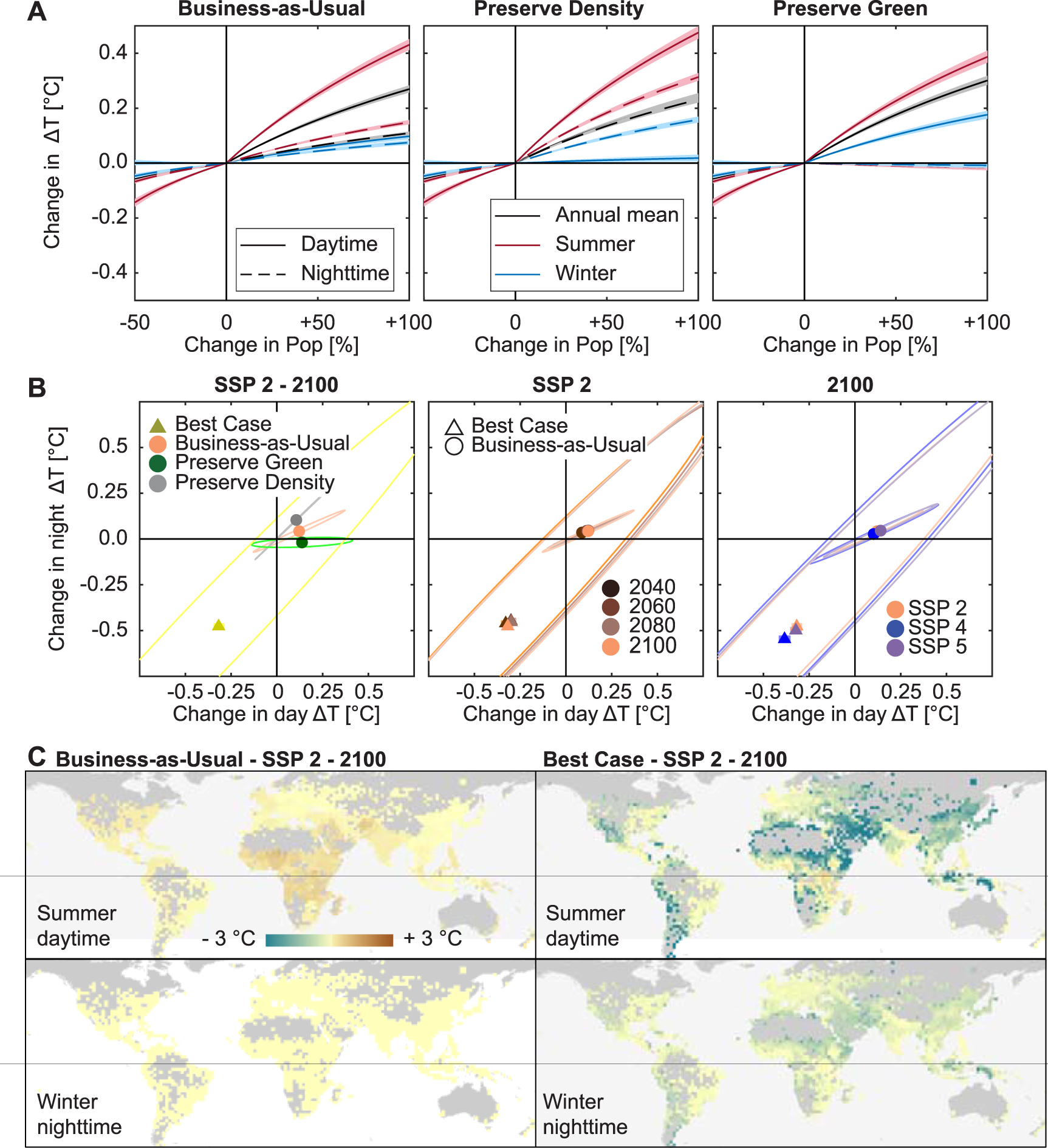
Figure 4(A) uses the coefficients from our model to show how the Business-as-Usual scenario and its variants affect future urban surface temperature anomalies ΔT. This non-geographially-explicit estimate offers a simple illustration of how basic urbanization parameters impact urban ΔT for the same amount of population growth. For comparison, population increase alone, without considering changing infrastructure, causes average warming of +0.14 ∘C (0.13, 0.16) during daytime in Summer for a doubling in population; this is only one third of the expected change in the Business-as-Usual scenario (+0.43 ∘C (0.41, 0.45)), illustrating that surface energy balance changes caused by infrastructure, and not population density, drives ΔT. This is comparable to the results from Manoli et al (2019) who linked urban heat to climate and population and modeled an increase in urban heat of approximately +0.52 ∘C for a doubling of population, not separating population and infrastructure. The Preserve Density and Preserve Green variants result in similar summer daytime ΔT increases (+0.48 ∘C (0.45, 0.50) and +0.39 ∘C (0.37, 0.41), respectively), but the different effects of built-up area and green space emerge in nighttime and winter ΔT, indicating a potential for divergent local preferences. In all cases the logarithmic relationship between population density and urban ΔT means that surface temperatures in less densely populated areas are expected to rise at a faster rate than already highly populated regions for the same influx of people. Accordingly, the densification of suburbs is expected to have significant impact on local temperatures and for hotter climates might increase populations surface temperature exposures. However, we must note that our pixel-base analysis does not describe any extension of the urban conglomerate (in comparison to Seto et al (2011), Liu et al (2020)) and is not intended to model urbanization in previously undeveloped lands.

Figure 4. (A) Expected changes in urban surface temperature anomalies (ΔT) for a change in population density following all urbanization scenarios. (B) Average change from current annual mean ΔT for different scenarios, years, and SSPs. The 90% confidence ellipse displaying spatial variability is given in lighter colors, the uncertainty for the mean point following the regression is given as a colored-in square. Changes during Summer and Winter are shown in figure S14. (C) Changes from current ΔT based on scenarios Business-as-Usual and Best Case. Average of all inner-city pixels in each 2∘ grid cells is shown.
Download figure:
Standard image High-resolution imageWe more formally and realistically implement these scenarios using geographically-explicit population projections from the shared socioeconomic pathways (SSPs) (O'Neill et al 2013, Riahi et al 2017) (figure 4(B), see supplement S2.6 for details). This geographic specificity allows us to add a second future scenario, Best Case, which implements the Mitigation measures described above on top of the Business-as-Usual scenario based on the precipitation projections of RCP 4.5 (Meinshausen et al 2011, Thrasher et al 2012) (this requires geolocation, as mitigation measures are locally-specific depending on local NDVI, precipitation and population density, see supplement S2.7). We project that Business-as-Usual urbanization under SSP 2 Middle of the Road will result in an increase in population-weighted urban summer daytime ΔT of 0.22 ∘C (−0.04, 0.66). 68% of this increase will occur by 2040 and 95% by 2060 (figure 4(B)(center)), although it is important to note that SSP 2 has the slowest increase in urban population of all of the SSPs (figure S12). In comparison, SSP 4 Inequality and SSP 5 Fossil-fueled development have much steeper early increases in urban population, and the total urban population of SSP 5 in 2100 is slightly higher than for SSP 2 and SSP 4 (respectively). Projected ΔT changes reflect this rank ordering at the end of the century (figure 4(B)(right)). For all scenarios, pathways, and years, urban summer daytime ΔT are projected to increase significantly more than all other times (figure S14), with small-to-negligible winter nighttime changes.
The Preserve Green and Preserve Density variants show that basic siting and zoning decisions may offer only minimal control over future urban ΔT, but our Best Case scenario suggests that much larger gains can be made by implementing best practices for greening and surface albedo (figure 4(B)(left)). Under this scenario and SSP 2, we find a decrease of surface daytime summer urban temperatures of −0.24 ∘C (−2.68, 0.33) or even −0.32 ∘C (−2.35, 0.40) when weighted per person. However, this potential for cooling is not universal, and even this Best Case scenario projects urban surface temperatures to increase in central Africa, and the Philippines (figure 4(C)). Additionally, cooling might only be projected for some parts of a city (e.g. figure S15), a key concern when inequality is already rife within cities (figure S4). However, the scenario projects no significant changes in within-city standard deviation in ΔT during daytime in summer (figure S16).
Maps of all Scenarios, years, and SSPs are shown in figures S17–S19, and show that projected differences are more strongly driven by urbanization strategy than SSP. While all pathways predict significant warming in Africa and Central Asia, the increase following scenario Business-as-Usual in these regions varies from approximately 0.7 to more than 1 ∘C. SSP 5 notably projects a significant warming for the USA and Canada and countries of the European Union.
Our results generally agree with the findings from previous, comparable studies: urban air temperatures in the USA are expected to increase between 0.3 and approximate 0.6 K due to urban densification by the end of the century (Krayenhoff et al
2018) and the urban effect to heat exposure is projected to increase by  10% (Broadbent et al
2020) (compared to a an increase in surface ΔT of approximately 0.2 ∘C–0.3 ∘C (5% to 10%) for summer days following our Business-as-usual scenario). Focusing on land expansion only a global regression model projected citywide warming of as much as 0.5 ∘C in the next 50 year for summer daytime temperatures (Huang et al
2019)—more than double our projections for surface temperatures and densification. We suspect that these differences are caused by high temperature increases in so far low built-up suburbs as discussed before. In this case absolute temperatures will likely still be lower than in the city center. Focusing on the effects of atmospheric forcing a recent study by Zhao et al (2021) projects urban (atmospheric) warming of 0.7–6.8 K by 2100 during summer depending on the region and RCP scenario—considerably higher numbers than the here projected effects of urbanization on surface temperature.
10% (Broadbent et al
2020) (compared to a an increase in surface ΔT of approximately 0.2 ∘C–0.3 ∘C (5% to 10%) for summer days following our Business-as-usual scenario). Focusing on land expansion only a global regression model projected citywide warming of as much as 0.5 ∘C in the next 50 year for summer daytime temperatures (Huang et al
2019)—more than double our projections for surface temperatures and densification. We suspect that these differences are caused by high temperature increases in so far low built-up suburbs as discussed before. In this case absolute temperatures will likely still be lower than in the city center. Focusing on the effects of atmospheric forcing a recent study by Zhao et al (2021) projects urban (atmospheric) warming of 0.7–6.8 K by 2100 during summer depending on the region and RCP scenario—considerably higher numbers than the here projected effects of urbanization on surface temperature.
6. Implications
We aggregate global population exposures under these different scenarios, present and future, to better understand the human implications of urbanization strategies. Key surface temperature thresholds under each scenario are shown in figure 5. The chosen limits are based on thresholds defined for daily surface air temperatures or a heat index (combining temperatures and humidity) where they give insight on the health and well-being of the urban population, and on the overall efficiency of cities in terms of both human labor productivity and energy demands. Here, assessing seasonal mean surface temperatures, we use them to illustrate the number of people living under extreme heat for our different scenarios.

Figure 5. (A) Distribution of urban population and surface temperatures they are exposed to. Distributions of present population are compared to hypothetical scenarios without ΔT and our optimized scenario Mitigation. Comparisons also include the future scenarios Business-as-Usual, which preserves present urban relationships into the future, and Best Case, which optimizes vegetation and albedo. Future population distributions are derived from SSP 2 for the year 2100. (B) The number of urban individuals living in areas with extremely hot summer days ( 35 ∘C), extremely hot summer nights (
 20 ∘C), winter heating degree days (HDD: 18 ∘C minus average temperature), and summer cooling degree days (CDD: average temperature minus 18 ∘C). These thresholds are typically applied to air temperature or a heat index not LST and can only be used here to compare scenarios. Percentages shown are relative to current.
Download figure:
Standard image High-resolution image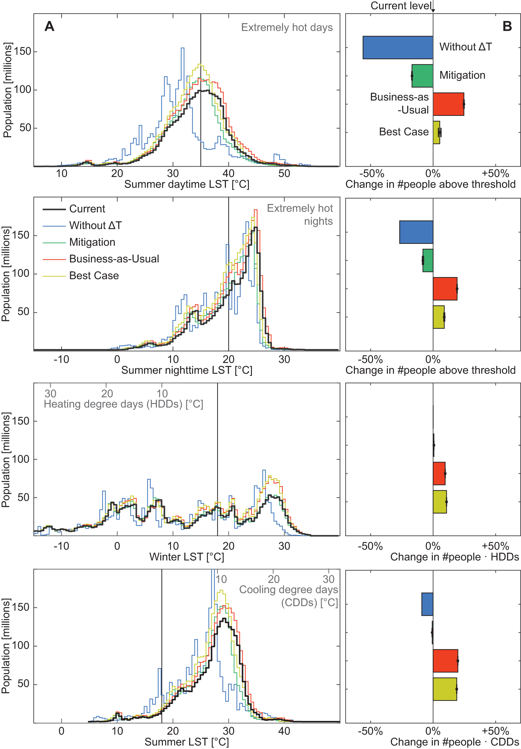
Without present, urban-induced alterations to the surface energy balance the number of urban individuals experiencing extremely hot days (average temperatures over 35 ∘C) would be reduced by 56.0%, and the number experiencing extremely hot nights (temperatures over 20 ∘C) by 26.8%. The short-term Mitigation scenario reduces the number of affected people by −16.88% (−17.11, −16.77) for extremely hot days and by −8.15% (−8.55, −7.68) for nights. In the longer run, the combined effects of population increases and Business-as-Usual urbanization patterns would increase the number of people over the threshold for extremely hot days by 24.68% (24.89, 24.48) and for extremely hot nights by 19.18% (19.08, 19.26). Although ΔT is mostly reduced in the Best Case scenario, the number of people will still increase due to the increase in population living in cities—5.29% (4.27, 6.29) for extremely hot days and 8.93% (8.58, 9.30) for extremely hot nights. This increased future population however lives in fewer urban pixels—following the Best Case scenario −13.04% (−13.76, −12.34) fewer urban pixels will have an average summer daytime temperature of over 35 ∘C (figure S20).
Importantly, these future urban surface temperature changes would be in addition to climate change-driven alterations to the surface energy balance that will affect rural and urban locations alike. Previous studies quantified atmospheric urban heat to be about half or even equally as impactful as global climate change (Estrada et al 2017).
Focusing on heating and cooling degree days (HDD and CDD) with a base temperature of 18 ∘C we find that ΔT increases the product of CDDs and population at present by 9.07% (see supplement S3 for an in-depth discussion).
To highlight the benefit of the pixel-based analysis we ran the same model based on city average surface temperatures and satellite measures (figure S21). We find that the city-based analysis severely underestimates the potential for mitigation as evident in the change in population experiencing extremely hot days following our scenarios Mitigation (pixel-based −16.88%; city-based −9.75%) and Best Case (pixel-based +5.29%; city-based +11.16%). At the same time the city-based analysis slightly underestimates projected future warming following our Business-as-Usual scenario (pixel-based +24.68%; city-based +21.52%).
7. Conclusion
Our data on local surface temperature anomalies and the analyses presented here show that the land cover changes associated with urbanization have a large effect on the surface temperatures urban populations are exposed to. Our findings are broadly consistent with prior analyses (Chakraborty and Lee 2019) (figure S22), but reveal new, important details of within-city heterogeneity, and widespread potential for mitigation. Moreover, we show that observable measures of the surface energy balance explain much of the variation in the urban surface temperature anomalies. At the kilometer-scale, urban surface temperature anomalies are less related to population densities than to the characteristics of local infrastructure and vegetation. On this basis we developed scenarios for mitigation and future urbanization. Uncertainty given with these scenarios only represents uncertainties in the estimate, not in the input parameters, particularly LST and projected population. These measurement errors are expected to translate into wider error bars, but not skewed error bars. They have therefore no significance when comparing different scenarios. Our results are summarized in figure S23: already surface urban temperature anomalies have doubled the number of people living in extreme land surface heat—depending on local conditions such as humidity this indicates higher air temperatures and increased risk for heat related illnesses. Without changes in urban planning (i.e. Business-as-usual), we project this number will further increase by up to 25% as of 2100. However, if locations with below-average vegetation and lower-than-average surface albedo were to alter local condition to meet the global average, we estimate that future (2100) urban surface temperature anomalies would decrease for 67% (65%, 68%) of the urban population. Nonetheless, these aggregate numbers belie substantial and important local differences: For example, our model consistently predicts additional urban warming in low-income Central African Countries and we find no indication that existing inequities of urban heat and hence health, comfort and productivity within single cities will decrease. Future work may focus on within-city patterns in greater detail and higher resolution, as they may be critical for city managers and urban planners working to redress socio-economic inequities and prepare their cities for the warmer world.
Data availability statement
All data, results and codes (Google Earth Engine and MATLAB R2018a) are openly available at the following URL/DOI: https://doi.org/10.6075/J0G44NQZ (Benz et al 2021). Location specific ΔT (including city averages) are accessible as a google earth engine app at https://sabenz.users.earthengine.app/view/surface-delta-t.
Acknowledgments
S A B is supported by the Big Pixel Initiative at UC San Diego, J A B, S J D, and S A B are supported by NSF/USDA NIFA INFEWS T1 #1619318; J A B is supported by NSF CNH-L #1715557. We would further like to thank three anonymous reviewers for their helpful comments.