

Abstract
In this study, we propose a new Arctic climate change indicator based on the strength of the Arctic halocline, a porous barrier between the cold and fresh upper ocean and ice and the warm intermediate Atlantic Water of the Arctic Ocean. This indicator provides a measure of the vulnerability of sea ice to upward heat fluxes from the ocean interior, as well as the efficiency of mixing affecting carbon and nutrient exchanges. It utilizes the well-accepted calculation of available potential energy (APE), which integrates anomalies of potential density from the surface downwards through the surface mixed layer to the base of the halocline. Regional APE contrasts are striking and show a strengthening of stratification in the Amerasian Basin (AB) and an overall weakening in the Eurasian Basin (EB). In contrast, Arctic-wide time series of APE is not reflective of these inter-basin contrasts. The use of two time series of APE—AB and EB—as an indicator of Arctic Ocean climate change provides a powerful tool for detecting and monitoring transition of the Arctic Ocean towards a seasonally ice-free Arctic Ocean. This new, straightforward climate indicator can be used to inform both the scientific community and the broader public about changes occurring in the Arctic Ocean interior and their potential impacts on the state of the ice cover, the productivity of marine ecosystems and mid-latitude weather.
Export citation and abstract BibTeX RIS
1. Introduction
Sea ice retreat in the Arctic Ocean is now recognized as a sensitive indicator of climate change (US Environmental Protection Agency Report, Climate Change Indicators in the United States 2012). Equally important, but not as widely recognized, is that the Arctic Ocean's halocline—the layering of fresher and lighter waters above saltier and denser waters below—is the fundamental structure that allows an ice cover to form (Nansen 1902). Indeed, most sea-ice loss results from atmospheric forcing, and surface air temperature has rightly been selected as an important indicator of Arctic change. However, recent ice reduction and shoaling of the intermediate-depth (∼150–800 m) Atlantic Water (AW) layer in the eastern EB of the Arctic Ocean have increased vertical mixing and upwards heat flux in ocean interior, making this region's conditions more similar to those of the western EB (Polyakov et al 2017). The associated enhancement of oceanic heat flux has reduced winter sea-ice formation at a rate comparable to the sea-ice loss due to atmospheric thermodynamic forcing, explaining the recent reduction in sea-ice cover in the eastern Arctic. This encroaching 'atlantification' of the eastern Arctic Ocean represents an important step toward a new Arctic climate state, one with potentially ice-free summers, and with a substantially greater role of Atlantic inflows.
This recently recognized role of halocline strength governing communication between the Arctic Ocean interior and its upper ocean and ice cover has not, surprisingly, yet been identified as a climate indicator. In this study, we thus propose a new Arctic climate change indicator that describes the variability in the strength of the Arctic halocline (figure 1) and provides a measure for vulnerability of sea ice to upward heat fluxes from the ocean interior.

Figure 1. The Atlantic/Pacific halocline front that separates the Amerasian and Eurasian halocline systems: the shaded ovals show the two halocline domains (from Carmack et al 2016, John Wiley ©2015. American Geophysical Union. All Rights Reserved). Color is used to show temperature and isolines are used to show salinity.
Download figure:
Standard image High-resolution image2. Data
We here use Arctic Ocean water column observations collected from 1981 to 2017; temporal and spatial data coverage is shown in figures S1–S5 available online at stacks.iop.org/ERL/13/125008/mmedia. This is an update of the archive of data used previously to describe long-term changes in the AW temperatures and Arctic freshwater content changes (e.g. Polyakov et al 2004, 2008, 2013). Aircraft and ship expeditions and year-round ice-drift stations provided data from the 1980s. Most of these observations prior to the mid-1980s were made using Nansen bottles and reversion thermometers. Typical measurement errors are 0.01 °C for temperature and 0.02 for titrated salinity. In the 1990s, icebreakers and submarines began to provide modern, high-quality measurements covering vast areas of the central Arctic Ocean. A significant increase the oceanographic observations was achieved in the 2000–2010s (figure S1). Ship-based summer measurements in the 2000s were complemented by ITP (Ice-Tethered Profilers; see www.whoi.edu/itp) drifters, to provide year-round CTD (conductivity-temperature-depth) measurements in the upper ∼800 m. CTD/ITP instruments have good vertical resolution and high accuracy of temperature (0.001 °C) and salinity (0.003 psu) measurements.
3. Methods
3.1. Halocline definition
The water column in the EB is characterized by a ∼20–50 m thick surface mixed layer (SML) overlaying the halocline which is divided into the cold halocline layer (∼50–100 m), distinguished by homogeneous near-freezing temperatures and the lower halocline waters (∼100–200 m) with increasing temperature and salinity with depth, until they reach AW (figure 1, e.g. Rudels et al 1991). In the AB the lateral injection of relatively fresh Pacific-origin waters at intermediate (60–220 m) depths further strengthens stratification to inhibit heat exchange between the AW and the SML (McLaughlin et al 2004, Steele et al 2004). Thus, the complex Arctic pycnocline is comprised of both salt (halocline) and temperature (thermocline) components, and the former dominates oceanic stratification.
For each CTD and ITP profile we identify the depth HSML of the SML, which is also the upper halocline boundary, by a change in water density from the ocean depth level closest to the surface of 0.125 kg m−3, following Monterey and Levitus (1997). The depth Hhalo of the lower halocline boundary is calculated following Bourgain and Gascard (2011) where it was argued that the density ratio Rρ = (α∂θ/∂z)/(β∂S/∂z) = 0.05 (α is the thermal expansion coefficient and β is the haline contraction coefficient, θ is potential temperature and S is salinity) may be used to mark the depth of the halocline base. This definition assumes that oceanic layers above Hhalo are almost entirely salt-stratified with very little contribution from temperature (as reflected in β∂S/∂z exceeding α∂θ/∂z by an order of magnitude). The halocline thickness is then defined as ΔHhalo =Hhalo − HSML.
3.2. Making regional composite time series
Regions selected for our analyses are presented in figure 2. The regional time series (figure 3) are constructed using techniques similar to those used for analysis of long-term AW and freshwater content variability (Polyakov et al 2004, 2008). In order to reduce effect of spatial non-homogeneity, the area of each region was divided into boxes matching 0.25° (latitude) × 0.75° (longitude) grid and individual parameters derived from CTD or ITP profiles were first averaged within a given month and box. Spatial averaging within each grid box using simple averaging of all points or distance-weighted averaging showed little difference (not shown, the latter was used in our analyses). Using these box-averaged monthly mean values, we computed seasonal cycle for each grid box and de-season original values of all individual parameters. Next, these de-seasoned values were spatially (within each box) and temporally (for each year) averaged to produce annual time series for each grid box where data are available. The resulting set of gridded time series for each box was averaged, taking into account the area of each box, to obtain a single time series for each region. This technique provides an accurate spatial representation of area-averaged indices, since these results are less skewed by non-homogeneity of spatial data coverage (see Polyakov et al 2004, 2008 for details).
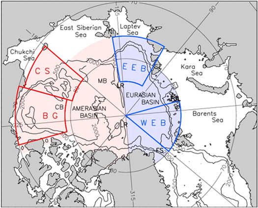
Figure 2. Arctic Ocean map with identified regions. Pink (blue) color is used to identify Amerasian Basin (Eurasian Basin). Eastern Eurasian Basin region (EEB), western Eurasian Basin region (WEB), Beaufort Gyre region (BG), and Chukchi Sea region (CS) are shown. The Lomonosov Ridge (LR), Novosibirskiye Islands (NI), Severnaya Zemlya (SZ), Franz Joseph Land (FJL), Makarov Basin (MB), and Canada Basin (CB) are indicated.
Download figure:
Standard image High-resolution image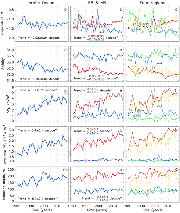
Figure 3. Annual pan-Arctic and regional halocline potential temperature θhalo, salinity Shalo, across-halocline potential density difference Δσθ, available potential energy APE, and depth of halocline base Hhalo. Solid lines connect dots with no gaps in between whereas dashed–dotted lines are used to fill gaps. Dashed or dotted lines show standard errors at 95% confidence level; errors for regional time series are shown in figure S6. In (b), (e), (h), (k), (l)) red lines are used for AB and blue lines are used for EB. In (c), (f), (I), (l), (k)) blue, green, yellow, and red lines are used for EEB, WEB, CS, and BG regions, respectively.
Download figure:
Standard image High-resolution image3.3. Characterizing stratification
Stratification within the SML and halocline layer may be quantified using Brunt–Väisälä buoyancy frequency (N), N2 = –(g/ρo)∂ρ/∂z, where ρ is the potential density of seawater, ρo is the reference density (1030 kg m−3), and g is the acceleration due to gravity. This parameter yields a detailed profile of stability between points in the vertical used to define vertical gradients, but does not yield an overall, bulk measure for the entire layer. When defined by density gradient between just two vertical points from the upper and lower halocline boundaries, the N2 is noisy. In addition, change of N2 results from both variations of density contrast between two vertical levels Δσθ, and from the vertical stretching of halocline layer ΔHhalo. N2 and Δσθ provide similar spatial patterns (not shown), but maps of N2 are noisier and we chose Δσθ for large-scale mapping purposes.
While buoyancy frequency N2 and density contrast Δσθ are reasonable measures of stability within the water column, they do not provide a bulk metric. The Arctic Ocean halocline is a complex layer, consisting, in general, of several different water masses and source regions (Bluhm et al 2015); yet neither N2 or Δσθ provide information about overall changes in halocline structure. Available potential energy (APE), however, is a good integral indicator of changes in overall halocline and SML strength. For each profile, it is calculated as
where z2 is the surface and z1 is the depth of the halocline base, g is the gravity acceleration, ρref is potential density at the base of the halocline, and z is depth.
3.4. Mapping
Spatial distributions of oceanic parameters over selected periods of time are presented in figure 4 as individual colored circles with values taken directly from data profiles, thus avoiding additional errors associated with spatial interpolation. However, comparison of evolution between different time periods is made using spatially interpolated data. Another possibility would be to use pairs of closest stations found within a search radius but our tests showed that this approach does not provide unique results (depending on what period of time is selected as the base one), especially for sparsely distributed observations; for that reason we used spatially interpolated data. For interpolation and presentation of differences between time periods we used 0.25° × 0.75° grid. Results are shown in figure 4.
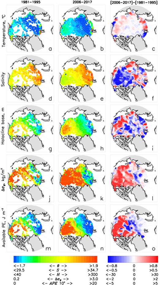
Figure 4. Averaged over the 1981–1995 (left column), 2006–2017 (middle column), and their difference (right column) of halocline (a)–(c) θhalo, (d)–(f) Shalo, (g)–(i) Hhalo, (j)–(l) Δσθ, and (m)–(o) APE.
Download figure:
Standard image High-resolution image4. Changes of Arctic halocline temperature, salinity, stratification, and thickness
We next analyze both pan-Arctic and regional changes in the upper Arctic Ocean to find the best available climate indicator illustrating the strength of Arctic halocline. For this purpose, annual time series of potential temperature θhalo, salinity Shalo, Δσθ, APE, and Hhalo are shown in figure 3. Spatial distributions of these parameters are averaged over 1981–1995 and 2006–2017 and their differences complement time series (figure 4). Analysis is carried out for 1981–2017, which is sufficiently long to capture climate related change, which has relatively good data coverage and which overlaps with the satellite observational period.
Here we provide a brief overview of changes occurring in the Arctic halocline since 1981. Noting that temperature does not contribute much to the halocline stability but for completeness of the description, we show that over almost four decades, θhalo did not show much changes in the AB, whereas in the EB observations demonstrate statistically significant cooling dominated by processes in the western EB (figure 4). Freshening of the upper AB is well documented (e.g. Proshutinsky et al 2009, Carmack et al 2016). Our observations complement these earlier findings by providing a quantified and statistically significant trend of continuous freshening of the AB halocline (figure 3). Shalo in the western EB shows little trend whereas in the eastern EB the late 1990s became a turning point from halocline freshening to salinification (figure 3). Distribution of Shalo difference between the earlier and later time intervals shows that the signal captured by the regional time series is spatially homogeneous in the AB and rather patchy in the EB (figure 4). We note here that changes in Shalo are readily transferrable to freshwater content changes.
Two parameters—Δσθ and APE—are used here to document changes in stratification of the upper Arctic Ocean. Figure 4 demonstrates that spatial patterns of Δσθ and APE (including their evolution in time, figures 4(l) and (o)) are similar showing very contrasting changes in two major Arctic Ocean basins associated with strengthening of stratification in the AB (positive values) and overall weakening in the EB (negative values). This spatial pattern is partially related to changes of the depth of the halocline base when the deeper the halocline's base, the more stable the water column is. This relationship is confirmed by high correlation (R = 0.75 for both AB and EB) between regional time series of APE and Hhalo. The trend towards stronger stratification in the upper AB is consistent with continued freshening in this region and deepening of the surface fresh layer due to intensification of Arctic high and wind-driven convergence of the upper ocean currents (e.g. Proshutinsky et al 2009, McPhee et al 2009). Contrasting changes in the upper EB are also consistent with the recent findings of 'atlantification' in the eastern EB (Polyakov et al 2017).
At the same time, regional time series of Δσθ and APE show differences (figures 3(k), (n)). Time series of APE clearly show distinct tendencies in the AB where the trend towards stronger stratification is steady, and statistically significant, whereas the EB is associated with small overall changes. The Δσθ records are noisier with high-level of high-frequency variations. Moreover, the distinction between the AB and EB time series is not as clear as shown with APE despite a similar tendency of higher and statistically significant trend of Δσθ in the AB and smaller and insignificant trend on the EB.
5. Synthesis
Upon comparison of two measures of the upper ocean stability, Δσθ and APE , we note that while these two parameters are complementary, we conclude that APE is somewhat superior for the objectives of this study (figures 5(a)–(c)). Consequently, we propose that this parameter be used as a climate change indicator in the Arctic. We note, however, that regional APE contrasts between AB and EB are striking whereas pan-Arctic time series of APE which does not take into account basin-wide structural differences (see Bluhm et al 2015) is not reflective of important regional contrasts (compare figures 5(a) with figures 5(b), (c)). Thus, we argue that the use of two time series, APEAB and APEEB—as an indicator will provide a powerful tool for detecting and monitoring progression of the Arctic Ocean towards new climate states.
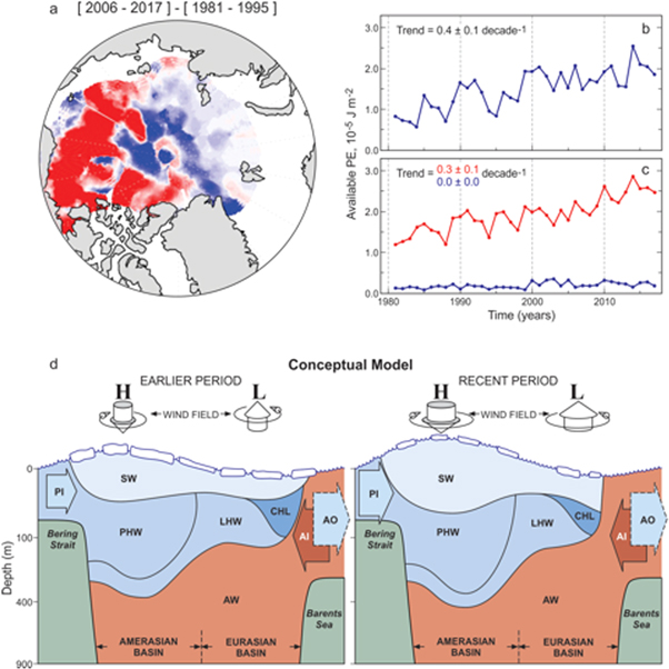
Figure 5. Strength of Arctic halocline illustrated by the APE as an indicator of Arctic Ocean climate change. (a) Map showing APE difference between two selected periods of time. (b), (c) Time series showing APE averaged over (b) the entire Arctic Ocean and (c) Amerasian (red) and Eurasian (blue) basins. (d) Conceptual model of change of Arctic halocline strength showing: (i) decrease in time of sea ice, (ii) enhanced impact of Arctic High on ocean circulation, (iii) increase of thickness of SML and halocline in the AB and decrease in the EB, (iv) increase of influx of Pacific Water (PI), (v) reduction of EB halocline.
Download figure:
Standard image High-resolution image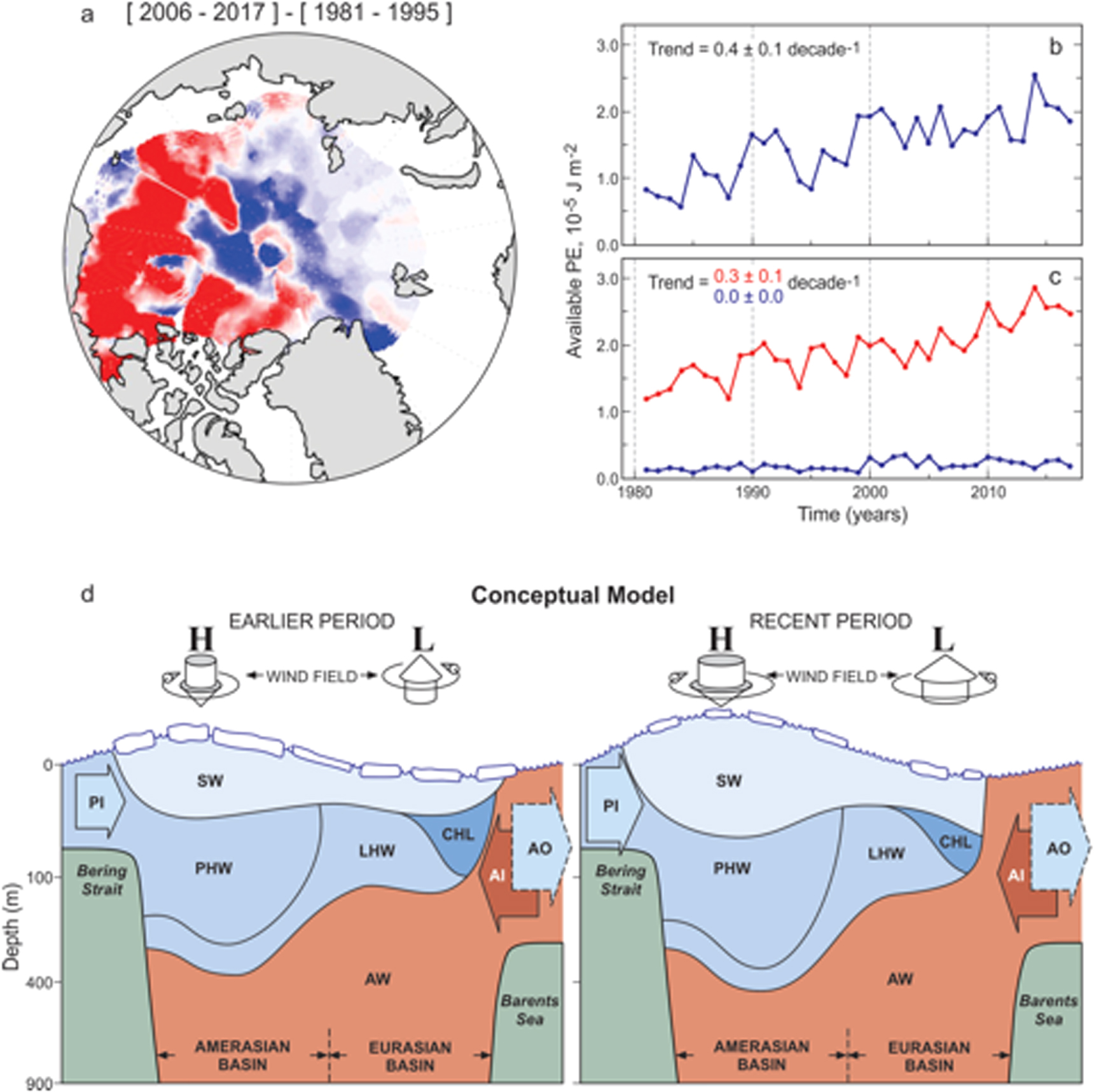
6. Conclusions
The proposed Arctic Ocean climate change indicator is responsive to the criteria used for the US National Climate Indicators System (Kenney et al 2016). For example, in our analysis we provided a solid scientific basis for the new indicator and thus we argue that it is scientifically relevant and defensible, and is based on sustained data sourses. The lack of such an indicator represents a serious gap in the list of global climate change indicators developed by the US Global Change Research Program (USGCRP).
The potential significance of the proposed Arctic climate change indicator is far reaching. In addition to providing fundamental knowledge regarding the dynamics of the Arctic halocline (figure 5), this indicator will provide impetus for improved representation of Arctic sea-ice responses to halocline changes in climate models. It may serve as a measure that delivers lead warning of impending changes in Arctic Ocean water mass structure and potential impacts on ice cover, upper ocean biology related to light and nutrient availability, and impacts on human activities (fisheries, shipping) and mid-latitudes. Further, the proposed indicator provides a foundation for the development of further hypotheses about Arctic climate system functionality. Thus, the proposed indicator will be an important contributor to the existing sets of Arctic climate change indicators.
Acknowledgments
Analyses presented in this paper are supported by NSF grants AON-1763343, AON-1534161, AON-1338948, AON-1203473, and 1708427. This paper is based in part on ideas discussed at an international workshop on pan-Arctic marine systems in Motovun Croatia, organized by P Wassmann and supported by funding from Arctic SIZE (http://site.uit.no/arcticsize/).