

Abstract
State and regional climate policies in the United States are becoming more prevalent. Quantifying these policies' health co-benefits provides a local and near-term rationale for actions that also mitigate global climate change and its accompanying harms. Here, we assess the health benefits of a carbon fee-and-rebate policy directed at fuel use in transport, residential and commercial buildings and industry in Massachusetts. We find that the air pollution reductions from this policy would save 340 lives (95% CI: 82–590), 64% of which would occur in Massachusetts, and reduce carbon emissions by 33 million metric tons, with 2017 as an implementation year, through 2040. When monetized, the benefits to health may be larger than the benefits from climate mitigation, but are sensitive to valuation methods, discount rates, and the leakage rate of natural gas, among other factors. These benefits derive largely from lower transportation emissions, including volatile organic compounds from gasoline combustion. Reductions in oil and coal use have relatively large benefits, despite their limited use in Massachusetts. This study finds substantial health benefits of a proposed statewide carbon policy in Massachusetts that carries near-term and direct benefit to residents of the commonwealth and demonstrates the importance of co-benefits modeling.
Export citation and abstract BibTeX RIS

Original content from this work may be used under the terms of the Creative Commons Attribution 3.0 licence. Any further distribution of this work must maintain attribution to the author(s) and the title of the work, journal citation and DOI.
Introduction
The transportation and building sectors contribute heavily to greenhouse gas emissions that drive climate change, and to other harmful air pollutants. In 2015, the transportation sector emitted 1700 million metric tons of CO2–32% of total US CO2 emissions. Residential and commercial buildings emitted 570 million metric tons of CO2–10% of total US CO2 emissions (US Environmental Protection Agency 2017). Road transportation is the largest contributor to air pollution-related mortality in the US (Caiazzo et al 2013), followed by electric power generation and commercial/residential buildings. Residential combustion alone has been associated with 10 000 deaths per year in the US (Penn et al 2017). Policies that mitigate climate change by reducing fossil fuel consumption can also have health benefits, often termed 'health co-benefits', by improving air quality (Wilkinson et al 2009, Nemet et al 2010, Perry et al 2014, Plachinski et al 2014, Mittal et al 2015, Thompson et al 2016, Haines 2017, Li et al 2018).
Research on co-benefits of carbon policies has found that health benefits can be substantial. The magnitude depends on sectors affected, policy design, and the geographical relationship between source locations and populations exposed to air pollution. In the electrical sector, health co-benefits are greatest for policies that principally displace coal (Siler-Evans et al 2012, Driscoll et al 2015, Buonocore et al 2015, 2016a, 2016b, Li et al 2018). Other studies have modeled hypothetical nation, state, or province-level carbon policies and found that policies targeting multiple economic sectors can have higher co-benefits than policies targeting just one sector, and that health benefits are generally higher if high-emission sources are reduced (Saari et al 2014, Thompson et al 2016, Li et al 2018). While these studies provide insight into drivers of benefits, they do not examine the benefits of specific state-level policies. This may become increasingly relevant, since with the proposed US withdrawal from the Paris Agreement, 11 states and 271 cities and counties have committed to actions that will meet or exceed greenhouse gas targets required to meet the Paris goals (Sanderson and Knutti 2016, Hepburn 2017, Tollefson 2017, we Are Still In n.d.).
Here, we assess the climate and health benefits of a model carbon fee-and-rebate bill applied to fossil fuel consumption in the transportation, residential, commercial, and industrial sectors in Massachusetts. The fee schedule starts at $10/ton in 2017, and increases by $5 yr−1, until it reaches a plateau price of $40 per ton in 2023, a price similar to many other carbon prices worldwide (Benson n.d., Barrett n.d., The World Bank n.d.). These bills, and our study, exclude electrical generation, since the electrical grid in Massachusetts is covered by the Regional Greenhouse Gas Initiative. We assess benefits from 2017 through 2040, assuming that the carbon price was implemented in 2017. We quantify the health co-benefits in economic terms and compare with monetized climate benefits.
Methods
We developed a model framework that links the following components (figure 1):
- CO2 emissions and fuel use reductions for Massachusetts from the Carbon Tax Assessment Model (CTAM).
- Emissions of SO2, NOx , PM2.5, and VOCs for relevant sectors within Massachusetts.
- A Community Multi-Scale Air Quality Model Direct Decoupled Method (CMAQ-DDM)-based impact-per-ton methodology providing state-resolution health benefits per ton of emissions reduced.
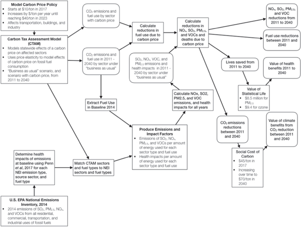
Figure 1. Flow diagram showing model components and linkages.
Download figure:
Standard image High-resolution imageUsing this framework, we estimated the reductions in fossil fuel use, CO2 emissions reductions, the reductions in emissions of NOx , SO2, PM2.5, and VOCs and the consequent health benefits, comparing a 'business-as-usual' (BAU) scenario with a policy scenario, put in monetary terms using standard valuation methodologies.
Modeling the reductions in fuel use and CO2 emissions
To estimate reductions in fossil fuel use and CO2 emissions, we used output from CTAM (Nystrom and Zaidi 2013, Breslow et al 2014). CTAM is an economic model that uses price elasticities, differing by fuel type and sector, along with state-specific economic data, including GDP growth, number of households, and existing policies, to estimate how fuel use will change, sector-wide, in response to changes in the price of the fuel. This model relies on future energy use forecasts from the National Energy Modeling System from the US Energy Information Administration, and existing literature on price elasticities of energy.
The carbon emissions from each fuel type and sector are calculated using standard emissions factors. The carbon fee is then applied to these carbon emissions under a BAU scenario, and the expected reduction in fuel consumption in response to the increase in price is calculated using the price elasticity—how fuel consumption changes in response to the change in price. From this fuel use reduction, we calculate the emissions reductions and health benefits of those reductions. To estimate the monetary value of the reductions in CO2 emissions, we use the social cost of carbon (SCC), a metric for measuring benefits of reducing carebon emissions, and put them in monetary, net-present-value terms. The specific values used here change over time to account for the increase in the marginal impact per ton of carbon emitted in future years, due to nonlinear response of the climate system to increased emissions. They start at $45 per ton (2017 USD) in 2017, and end at $70 per ton (2017 USD) in 2040 (Interagency Working Group on Social Cost of Carbon 2016). We present the benefits of CO2 reductions undiscounted and discounted at 3% yr−1, to be consistent with the discount rate of future impacts internal to each year's estimate of the SCC of an emission in that year.
Estimating reductions in emissions of non-GHG air pollutants, and health benefits
To estimate the reductions in PM2.5, SO2, NOx , and VOCs from the carbon fee-and-rebate policy, we used emissions data from the US EPA National Emissions Inventory (NEI) from 2014 as our BAU emissions. We used these emissions data along with the BAU fuel consumption from CTAM to create sector-and-fuel type-wide emissions factors for fuel use within Massachusetts. We then used these emissions factors to calculate BAU emissions in future years. The matching between CTAM and NEI fuel types and sectors are described in detail in the supplemental (table S1 is available online at stacks.iop.org/ERL/13/114014/mmedia). To estimate the health benefits of the emissions reductions, in terms of mortality avoided, we used a CMAQ-based impact-per-ton methodology that gives source state-resolution estimates of mortality avoided per ton of pollutant reduced, across multiple source sectors (Levy et al 2016, Penn et al 2017). CMAQ is a complex atmospheric chemistry, fate, and transport model that is often used by the US EPA to simulate the air quality impacts of air pollution and energy policies, and is commonly used for research purposes (Buonocore et al 2014, Stackelberg et al 2013, Roy et al 2007, Foley et al 2010, US Environmental Protection Agency, Office of Air Quality Planning and Standards, Air Quality Assessment Division 2012, Fann et al 2011, Appel et al 2017, Arunachalam et al 2011, Byun and Schere 2006).
This impact-per-ton methodology is based on a series of runs with the CMAQ-DDM (Levy et al 2016, Penn et al 2017). DDM allows for the influence of given emissions sources and pollutants across the modeling domain to be tracked within a given simulation (Napelenok et al 2006, Wagstrom et al 2008, Itahashi et al 2012). The impact-per-ton methodology used here was developed using CMAQ-DDM to individually model the sensitivities of ambient concentrations of PM2.5 and ozone to emissions of SO2, NOx , PM2.5, and VOCs in both winter and summer for multiple sectors within each source state in the US (Cohan et al 2005, Bergin et al 2012, Itahashi et al 2012, Levy et al 2016, Penn et al 2017). These sensitivities, providing estimates of the air quality impact per ton emitted for each precursor pollutant, were then used to model the health impacts using a concentration-response function of a 1% increase in all-cause mortality per 1 μg m−3 increase in annual average ambient PM2.5 levels (95% CI: 0.2–1.8) and a 0.4% increase in daily mortality per 10 ppb increase in ozone concentrations (95% CI: 0.14–0.66), population data from the US Census, and baseline mortality data from the Centers for Disease Control and Prevention. These concentration-response functions were similar to those used in previous studies (Roman et al 2008, Driscoll et al 2015, Levy et al 2016, Buonocore et al 2016a, Penn et al 2017, Centers for Disease Control and Prevention n.d., Bell 2004, Bell et al 2005, Schwartz 2005), and the 95% confidence intervals encompass the variability in concentration-response functions from major epidemiological studies of air pollution (Bell 2004, Bell et al 2005, Schwartz 2005, Lepeule et al 2012, Driscoll et al 2015, Levy et al 2016, Penn et al 2017). For transportation-related sources, we applied the average of the summer and winter sensitivities; for building-related sources, we used the sensitivities for winter, which assumes that most of the fuel use in these sectors is for heating (US Energy Information Administration 2018).
To put a monetary value on the lives saved from the emissions reductions, we used the value of statistical life (VSL) (Dockins et al 2004). This is a willingness-to-pay methodology commonly used in regulatory impact analysis and other policy research applications that captures most of the value of the health benefits from emissions reductions (Dockins et al 2004, US Environmental Protection Agency Office of Air Quality Planning and Standards 2011, Siler-evans et al 2012, Thompson and Selin 2012, Siler-Evans et al 2013, Thompson et al 2014, US Environmental Protection Agency, Office of Air and Radiation, Office of Air Quality Planning and Standards 2015, Thompson et al 2016, Buonocore et al 2016a). To account for the delay between PM2.5 exposure and mortality, we use a standard cessation lag (US Environmental Protection Agency Office of Air Quality Planning and Standards 2011, US Environmental Protection Agency, Office of Air and Radiation, Office of Air Quality Planning and Standards 2015). The VSL for PM2.5-related mortality is $8.5 million; the VSL for an ozone-related mortality case is $9.4 million, since there is not a significant lag between ozone exposure and mortality. We calculate the stream of health benefits both undiscounted and discounted at 3% yr−1, to be consistent with the values used in the SCC. All monetary values are presented in 2017 USD.
Results
Changes in fuel use and emissions reductions
Transportation had the highest reduction in energy use, followed by residential buildings. Gasoline was the fuel type with the highest reduction in use, followed by natural gas (figure 2). Reductions vary over time given the increasing carbon price through 2023, with differential responses to rising carbon prices among sectors. Peak reductions in motor vehicle gasoline use occur in 2025 and begin to decrease after 2025. For other affected sources, this peak occurs in 2035 (figure 2).
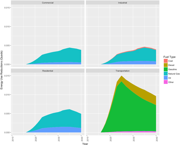
Figure 2. Reductions in fuel use due to a model carbon fee-and-rebate bill in Massachusetts, by source category and fuel type.
Download figure:
Standard image High-resolution imageThe air pollutant with the most reductions is NOx , followed by VOCs (figure 3(a)). Reductions in all air pollution emissions except VOCs grow rapidly until 2023, grow more slowly between 2023 and 2025, plateau or decrease between 2025 and 2035 (figure 3(a)); VOCs reach their peak in reduction in 2025 and taper off afterwards (figure 3(a)). The CO2 reductions follow a time trend where they reach a peak in 2025, plateau from 2025 to 2035, and then begin to taper off after 2035 (figure 3(b)). Reductions in NOx and primary PM2.5 emissions are largely from reduced use of gasoline, oil, and diesel in the transportation sector (figure 3(a)). Reductions in SO2 are largely from reduced oil use in residential and commercial buildings, and from reduced coal use in the industrial sector (figure 3(a)). VOC reductions are mostly from reduced gasoline use in the transportation sector (figure 3(a)). CO2 emissions reductions are largely driven by reductions in gasoline use in the transportation sector from implementation to 2025 (figure 3(b)). CO2 reductions from gasoline use taper off after 2025, while reductions from reduced natural gas use grow, becoming roughly equal to reductions from gasoline use in 2035 (figure 3(b)).

Figure 3. (a): Emissions reductions of NOx , PM2.5, SO2, and VOCs due to a model carbon fee between 2017 and 2040, by source sector and fuel type. (b): Emissions reductions of CO2 due to a model carbon fee between 2017–2040, by source sector and fuel type.
Download figure:
Standard image High-resolution imageEmissions avoided per unit of energy use reduced are very high for the use of oil in transportation, and high across all other sectors (figure 4(a)). Coal has the highest SO2 emissions reductions per unit energy reduced (figure 4(a)). Gasoline and diesel use in the transportation sector also had fairly high VOC emissions avoided per unit energy reduced (figure 4(a)). CO2 reductions per unit of energy reductions are much more even across fuel types and source sectors than for air pollutants (figure 4(b)).
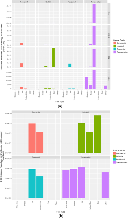
Figure 4. (a): Aggregate NOx , PM2.5, VOCs, and SO2 emissions reduced per unit energy consumption reduced, by source sector and by fuel type. (b): Aggregate CO2 emissions reduced per unit energy consumption reduced, by source sector and by fuel type.
Download figure:
Standard image High-resolution imageHealth and climate benefits
Between 2017–2040, this policy saves approximately 340 (95% CI: 82–590) lives (table 1, figure 5). The health benefits roughly parallel emissions reductions over time, with a value of $2.9 billion (95% CI: $0.71–$5.2 billion) undiscounted, and a value of $2.0 billion ($0.49–$3.5 billion) when discounted at 3% yr−1 (table 1, figure 6). The health benefits of this policy are mainly driven by NOx reductions contributing to both ozone and PM2.5, primary PM2.5, and emissions from VOCs, which contribute to both PM2.5 and ozone formation (figure 5). Reductions in SO2 emissions had a comparatively small contribution (figure 5). Emissions reductions in the transportation sector were the largest contributor (85%) to total health benefits, with health benefits initially driven by reductions in gasoline, but gradually becoming nearly evenly split among diesel, gasoline, and oil as the carbon fee goes into effect (figure 5, table 2). The lives saved mainly occurred within Massachusetts, with 63%, and in the surrounding states–12% in New Hampshire, 8% in New York, 4% in Rhode Island, 4% in Connecticut, 4% in New Jersey, and 2% in Maine (table 2).
Table 1. Total climate and health benefits of a carbon fee and rebate policy in Massachusetts from 2017–2040.
| Benefit type | Benefits (95% CI) |
|---|---|
| Total lives saved | 340 (82–590) |
| Value of health benefits, undiscounted | $2.9 billion ($0.66–$5.2 billion) |
| Value of health benefits, discounted at 3% yr−1 | $2.0 billion ($0.45–$3.5 billion) |
| Total reductions in CO2 emissions | 33 million metric tons |
| Value of climate benefits, undiscounted | $2.0 billion |
| Value of climate benefits, discounted at 3% yr−1 | $1.3 billion |
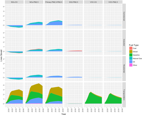
Figure 5. Lives saved per year due to a model carbon fee between 2017–2040, by emission type and resulting pollutant, by source sector, and fuel type.
Download figure:
Standard image High-resolution image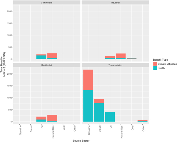
Figure 6. Aggregate monetized and undiscounted benefits of a carbon fee for different affected sectors (2017 USD), broken out by whether the benefits are due to climate mitigation or health, and by fuel type and source sector.
Download figure:
Standard image High-resolution imageTable 2. Proportion of health benefits from air pollution reductions from a carbon fee and rebate policy in Massachusetts from 2017–2040, by state and by source sector.
| Percentage of source sector benefits occurring within state | |||||||||
|---|---|---|---|---|---|---|---|---|---|
| Source sector | Total lives saved in all states | MA | NH | NY | RI | CT | NJ | ME | All others |
| Commercial | 7% | 57% | 14% | 10% | 4% | 5% | 4% | 4% | 2% |
| Industrial | 4% | 54% | 14% | 11% | 4% | 5% | 5% | 4% | 2% |
| Residential | 4% | 51% | 14% | 12% | 4% | 5% | 6% | 4% | 3% |
| Transportation | 85% | 65% | 12% | 7% | 4% | 4% | 3% | 2% | 3% |
| Total from all sectors | 63% | 12% | 8% | 4% | 4% | 4% | 2% | 3% | |
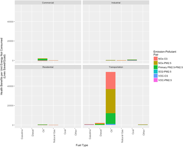
Reduction in oil use, largely in buildings and in transportation, also contributed highly to health benefits. Reductions in NOx emissions from buildings, largely from lesser oil and natural gas use, predominantly occurred in the winter and produced slight increases in ozone. This slightly reduced the total health co-benefits (figure 5). Reduced oil consumption for transportation also generally has the highest lives saved per unit of energy reduced, especially in transportation, but reduced coal use in industry is also high, largely driven by SO2 reductions (figure 7). When monetized, oil generally has the highest benefits per unit of energy consumption reduced, especially in transportation. Between 2017–2040, the policy would reduce CO2 emissions by approximately 33 million metric tons (figure 2(b)). The CO2 reductions have a value of $2.0 billion undiscounted, and $1.3 billion when discounted at 3% yr−1 (table 1, figure 2(b)).
Figure 7. Aggregate lives saved per unit energy consumption reduced, by source sector, fuel type, and emission type and resulting pollutant pair.
Download figure:
Standard image High-resolution image
The monetized benefits are slightly higher for health than for climate, with marked variation across sectors and fuel types (table 1, figure 6). The monetized benefits are largely driven by transportation, followed by the buildings sectors. The benefits of reduced fuel consumption in transportation were driven by health, with a more even split between health and climate for commercial buildings. Residential and industrial benefits were mostly based on greenhouse gas mitigation (figure 6). Across fuel types, the leading contributor to benefits is reductions in gasoline use, followed by diesel, oil and natural gas (figure 6). Health benefits generally contributed more to total benefits than climate for gasoline, diesel, and oil, while climate benefits were greater for natural gas than health (figure 6).
Discussion
A model carbon fee-and-rebate bill in the state of Massachusetts would advance greenhouse gas emissions' reductions, while providing substantive, health gains, mainly within state, that have comparable magnitude to the climate benefits when monetized.
The peak reductions occur after the peak price due to the time required for turnover, which is longer for buildings than the vehicle fleet. Reductions in fuel consumption and pollutant emissions reach a plateau and then fall since the model carbon fee is not tied to inflation.
Our results here indicate that when monetized, the health benefits are fairly similar in magnitude to the climate benefits, comparable to findings in previous studies focusing on renewable energy and energy efficiency (Siler-Evans et al 2012, 2013, Buonocore et al 2015, 2016b, Levy et al 2016). Between 2017–2040, this policy has approximately $88 in health benefits per ton of CO2 reduced, and saves 10.3 lives per million tons of CO2 reduced, similar to estimates from an economy-wide cap-and-trade program implemented in the northeast US (Thompson et al 2016), and slightly higher than a carbon standard in the electrical sector in the US (Driscoll et al 2015).
The model framework developed here has a number of limitations. The CTAM model does not fully capture spillover effects (like purchasing fuel out-of-state), effects of technology change, or effects of future regulations. There are a number of actions that can be taken to reduce emissions, including transportation mode-shifting, purchasing vehicles with higher fuel economy, and energy efficiency in buildings, but CTAM also does not model how the changes in fuel demand are being implemented, what the costs are, and which actors incur those costs (Washington State Department of Commerce n.d., Breslow et al 2014). CTAM does employ a lag structure in the price elasticity, so it is able to appropriately reflect longer-term changes due to, for example, turnover time of building stock or vehicle fleet (Washington State Department of Commerce n.d., Breslow et al 2014). Since CTAM does not explicitly model how the reductions in fuel use are occurring, it cannot model what changes are temporary and reversible, like switching from driving a personal vehicle to using public transportation or maintaining buildings at a lower indoor temperature; or permanent, like purchasing a more fuel-efficient vehicle or improving home insulation (Washington State Department of Commerce n.d., Breslow et al 2014). Future changes in emissions due to air quality regulations, changes in combustion efficiency or fuel mix, changes in the use of air pollution controls or other technology changes are not captured. While the use of CTAM and reliance on emissions from NEI may not capture all relevant economic, regulatory, and technological effects that may determine emissions reductions and health gains from a carbon price, the basic framework does reasonably at capturing the main drivers of the benefits of a carbon fee-and-rebate policy, including economic effects associated with price elasticity (Nystrom and Zaidi 2013, Breslow et al 2014). This modeling framework here is fairly similar to the economic modeling in previous studies (Thompson et al 2016, Li et al 2018). Although these studies contain more explicit linkages to other elements of the economy, linkages to trade, and other economic factors, while the model used here exclusively uses in-state changes (Thompson et al 2016, Li et al 2018). Use of CTAM alone is also insufficient to understand broader economic impact of a carbon policy, in part, because the economic effects of a carbon price depend on what is done with the revenue (Nystrom and Zaidi 2013, Breslow et al 2014, Ambasta and Buonocore 2018, California Air Resources Board 2018).
Our health model operates at state-level resolution with average values for winter and summer, so may not perfectly capture effect variability due to population proximity to sources, timing of emissions, or changes in population or baseline population health status over time. Across Massachusetts, the county-level mortality rate varies by a factor of two (872 to 1662 per 100 000), and the social costs of NOx , SO2, and PM2.5 emissions also do not vary substantially (Centers for Disease Control and Prevention n.d., Heo et al 2016a, 2016b). The model may still not perfectly capture possible geographical clustering of emissions reductions and areas with high population or more vulnerable populations, introducing some uncertainty. Additionally, the use of residential combustion impact-per-ton values is an imperfect proxy for transportation-related emissions, but the county-level emissions from each source type are reasonably correlated (Pearson correlation coefficients: 0.65 for SO2, 0.71 for VOCs, 0.73 for PM2.5, and 0.98 for NOx ).
Using emissions and impact rates from a historical base year to estimate the impacts of future changes in air pollution is common (Buonocore et al 2014, 2015, 2016a, 2016b, Driscoll et al 2015, Levy et al 2016, Heo et al 2016a, 2016b, 2017, Penn et al 2017). Ignoring population growth and aging would likely result in an underestimate of benefits. Technology changes over time could result in reduced emissions per unit energy and a corresponding overestimate of the total climate and health benefits. The model framework employed here does not have as high spatial and temporal resolution as other research, but our impact-per-ton functions are based on an advanced atmospheric modeling platform and allow for decomposition of benefits by sector and by emission type.
This analysis excludes several morbidities associated with air pollution including, like cardiovascular and respiratory disease, asthma, heart attacks, stroke, premature birth, low birth weight, lost days of school and work, and neurocognitive diseases (Gilliland et al 2001, Zanobetti and Schwartz 2009, Zanobetti et al 2009, Darrow et al 2010, Anderson et al 2011, Mustafić et al 2012, Levy et al 2012, Kloog et al 2012, Madrigano et al 2013, Jacquemin et al 2015, Talbott et al 2015, Jung et al 2015, Li et al 2016, Chen et al 2017, Cacciottolo et al 2017). We also do not include ecological benefits of reduced air pollution, like increased productivity for crops and timber, and decreases in eutrophication (Jaworski et al 1997, Aldy and Kramer 1999, Wittig et al 2007, Van Dingenen et al 2009), or health impacts from the reduction in hazardous air pollutant (Sunderland et al 2016). We also do not include other health and environmental impacts of extraction of the fuels whose use is avoided, including methane leaks from natural gas infrastructure, strain on underground natural gas storage facilities, air and water pollution and consequent health impacts from natural gas extraction, and possible impacts from accidents in oil and gas extraction or transportation (Adgate et al 2014, Brandt et al 2014, McKenzie et al 2014, Subramanian et al 2015, Brandt et al 2016, Peres et al 2016, Torres et al 2016, Butkovskyi et al 2017, Harriman et al 2017 , Michanowicz et al 2017).
The climate benefits may be quite sensitive to methane leakage across the natural gas supply chain. A leak rate of 2.3% and a social cost of methane of $1200 per ton would result in an additional ∼$138 million in benefits from climate mitigation, increasing the total benefits due to reduction in natural gas consumption by around 18% (Interagency Working Group on Social Cost of Carbon 2016, Phillips et al 2013, Alvarez et al 2018). Using the global average social cost of methane of $4600 per ton, which incorporates health impacts, makes benefits of reduced leakage closer to $530 million, or a 31% higher (Shindell 2015). Higher leakage rates, or higher weighting of near-term climate impacts would increase this sensitivity substantially. Our SCC may be an underestimate, as it may miss some important health impacts, effects on economic growth, and not appropriately deal with the distribution of climate impacts across space or time (Arrow et al 2013, Diaz and Moore 2017).
This study adds to existing literature on the health co-benefits of efforts to mitigate climate change. We examine the effects of a multi-sector fee-and-dividend bill, not including electricity, whereas much of the existing health co-benefits literature applies to electricity generation. It also examines an individual state plan, as opposed to regional or national policies. That said, the benefits of applying a carbon price to electricity generation can be around 3.9 lives per million tons of CO2 emissions reduced (Driscoll et al 2015). Another study examining nationwide clean energy standards found that the value of the health benefits can exceed the policy implementation costs (Thompson et al 2014).
With two years remaining to change the global trajectory of carbon emissions to meet the goals set forward by the Paris Agreement (Figueres et al 2017), and the US having announced its intent to leave the agreement (Tollefson 2017), regional, state, and local carbon pricing initiatives have become more important to the nation as a whole (Hepburn 2017). Understanding the health co-benefits of different policy options can aid in the design of policies, help incentivize their implementation (Petrovic et al 2014, Bain et al 2015), and help sub-national governments contribute to the world achieving the goals of the Paris Agreement.
Acknowledgments
We would like to thank Scott Nystrom at REMI for providing us with CTAM model output. We would like to thank: the Merck Family Fund and the Clean Water Fund, Ms Louise Hara and Mr Wayne H Davis, Mrs Susanna B Place and Mr Scott L Stoll, The Dante R Greco Trust, Ms Cynthia Margaret Iris and Mr Richard McFadyen, Mr Nagesh Mahanthappa, Mr John M Dacey, Mr James Recht and Nina Dillon, Zaurie Zimmer and Craig LeClair, Dr Richard Clapp, Dr Susan J Ringler, and Ms Bonni J Widdoes for their support for this study. The funders did not have a role in the design of the study, analysis of the model results, or preparation of this manuscript.