

Abstract
The decline in the floating sea ice cover in the Arctic is one of the most striking manifestations of climate change. In this review, we examine this ongoing loss of Arctic sea ice across all seasons. Our analysis is based on satellite retrievals, atmospheric reanalysis, climate-model simulations and a literature review. We find that relative to the 1981–2010 reference period, recent anomalies in spring and winter sea ice coverage have been more significant than any observed drop in summer sea ice extent (SIE) throughout the satellite period. For example, the SIE in May and November 2016 was almost four standard deviations below the reference SIE in these months. Decadal ice loss during winter months has accelerated from −2.4 %/decade from 1979 to 1999 to −3.4%/decade from 2000 onwards. We also examine regional ice loss and find that for any given region, the seasonal ice loss is larger the closer that region is to the seasonal outer edge of the ice cover. Finally, across all months, we identify a robust linear relationship between pan-Arctic SIE and total anthropogenic CO2 emissions. The annual cycle of Arctic sea ice loss per ton of CO2 emissions ranges from slightly above 1 m2 throughout winter to more than 3 m2 throughout summer. Based on a linear extrapolation of these trends, we find the Arctic Ocean will become sea-ice free throughout August and September for an additional 800 ± 300 Gt of CO2 emissions, while it becomes ice free from July to October for an additional 1400 ± 300 Gt of CO2 emissions.
Export citation and abstract BibTeX RIS

Original content from this work may be used under the terms of the Creative Commons Attribution 3.0 licence. Any further distribution of this work must maintain attribution to the author(s) and the title of the work, journal citation and DOI.
1. Introduction
Sea ice plays a critical role in the Earth's climate by regulating the exchanges of heat, momentum and moisture between the atmosphere and the polar oceans, and by redistributing salt within the ocean. Sea ice primarily exists in the polar regions, and throughout the observational record, at least 16 million km2, or about 5%, of the world's oceans have been covered by sea ice at any one time. Because of its high reflectivity, sea ice reflects the majority of the sun's radiation reaching the surface back to space, which efficiently cools the polar regions of our planet. As sea ice melts at its surface, its surface albedo is lowered, which in turn increases the amount of the sun's energy absorbed by the ice surface and further enhances ice melt. When the ice completely melts, this solar radiation is absorbed by the darker ocean surface, generating a positive feedback that amplifies Arctic air temperatures in autumn and winter as the ocean returns the heat gained in summer back to the atmosphere (e.g. Serreze et al 2009). This positive feedback process is one of the reasons why the polar regions react far more strongly to a rise in global mean temperature than most other parts of our planet, and it is part of the explanation for why the Arctic has warmed faster than the rest of the globe during the last few decades (e.g. Pithan and Mauritsen 2014, Huang et al 2017). In this review, we exploit state-of-the-art observational records and model simulations of polar sea ice to characterize and explain the recent wide-spread changes in the Arctic sea ice cover across all seasons.
Much of our understanding of Arctic sea ice changes comes from satellite retrievals with successive multichannel passive microwave sensors which began in October 1978. These allowed for continuous monitoring of sea-ice concentration (SIC) and total sea-ice extent (SIE), with Arctic-wide coverage every other day until July 1987 and every day from there onwards. Using this satellite data record, several studies have reported on the shrinking summer SIE since 1979 (e.g. Cavalieri and Parkinson 2012, Stroeve et al 2012a). Based on linear regression through the entire time series, these studies identified a nearly 14% per decade decline in the summer SIE. However, this trend has not been constant: the second half of the September SIE time series shows a trend about 3.5 times that of the first half (Stroeve et al 2012a, Serreze and Stroeve 2015). The decline during winter was much weaker, about −2.4% per decade.
The passive microwave satellite record has also been used to examine changes in the duration of the melt season and in the timing of ice retreat and advance (Markus et al 2009, Biss and Anderson 2014, Stroeve et al 2014a, 2016, Serreze et al 2016a). It was found that the pan-Arctic melt season is starting earlier by 3 days per decade and ending later by 6 days per decade, suggesting the seasonality of the ice cover is changing. Earlier ice retreat, driven in part by earlier melt onset, combined with later ice advance, has led to a lengthening of the ice-free season throughout the Arctic, with the largest increases of 40 days per decade found within the Barents Sea.
These examples indicate how useful the 40 year long, consistently processed passive microwave record has been to identify large-scale changes in sea-ice coverage. Unfortunately, similarly long-term records of ice thickness are not available and thus less is known about how the total mass of the sea-ice cover has changed in recent decades. The existing limited observations from upward looking sonars on submarines and moorings, laser and radar altimeters (satellite and aircraft), and other in situ observations nevertheless strongly suggest that the ice cover has not only shrunk in area, but that its average thickness has decreased from about 3.6 to 1.3 m over the period 1975–2012 (e.g. Lindsay and Schweiger 2015, see also Kwok and Rothrock 2009).
The Arctic sea-ice cover is also getting much younger, with the Arctic Ocean now primarily consisting of first-year ice, as opposed to the prevailing 5 year old multiyear sea ice during the early times of the satellite record (Maslanik et al 2007, Maslanik et al 2011, Stroeve et al 2012a). This is consistent with the observed thinning of the ice cover, as younger ice has had a shorter period of thermodynamic ice growth and thickening from deformation compared to older ice (Maslanik et al 2007, Tschudi et al 2016a).
Most of the observed changes in the sea-ice cover are driven by anthropogenic warming from increasing atmospheric greenhouse gas concentrations (e.g. Notz and Marotzke 2012, IPCC 2013, Notz and Stroeve 2016), amplified by internal variability (e.g. Ding et al 2017, Notz 2017). Notz and Stroeve (2016) quantified the relationship between the September SIE and cumulative atmospheric CO2 emissions, and emphasized the importance of limiting future CO2 emissions to those compatible with a global warming well below 2 °C in order to keep the summer ice cover. This urgency has been supported by more recent studies (Screen and Williamson 2017, Jahn 2018, Niederdrenk and Notz 2018, Sigmond et al 2018).
While complete loss of the summer sea-ice cover will have far-reaching implications beyond the Arctic, the observed reductions in sea-ice thickness and coverage are already impacting the energy balance of our planet. Expanding open water areas during summer have allowed for more absorption of heat into the ocean mixed layer, warming ocean temperatures and delaying autumn freeze-up (Stroeve et al 2014a). Before the ice can form again in winter, the ocean must release this heat back to the atmosphere. Large exchanges of heat and moisture from the ocean to the atmosphere have thus contributed to amplified winter warming of the lower troposphere in the Arctic (e.g. Serreze et al 2009), increased atmospheric moisture content of the Arctic atmosphere (Serreze et al 2012, Boivsert and Stroeve 2015), increased cloud cover (e.g. Jun et al 2016) and increased autumn precipitation (e.g. Kopec et al 2016). Warming from sea-ice loss has additionally been shown to impact permafrost temperatures (Lawrence et al 2008) and may have local impacts on Greenland melt (Stroeve et al 2017).
However, this amplified Arctic warming may trigger concurrent processes that can be felt not only by Arctic communities, but in communities around the world through its potential influence on large-scale weather patterns (e.g. Kretshmer et al 2016, 2017, Jaiser et al 2016, Sun et al 2016, Francis 2017, Screen et al 2018, Vavrus 2018), ocean circulation (Haine et al 2015) and enhanced ice sheet and glacier melt (Stroeve et al 2017) that lead to sea level rise. Consequently, understanding current and future sea ice loss will benefit people, policy, ecosystem management and businesses well beyond the Arctic.
This review provides an updated assessment of Arctic sea ice changes, with a broad perspective considering changes across all seasons. We combine insights from observational records, atmospheric reanalyses and large-scale climate-model simulations to assess the changing seasonality of sea ice conditions, its drivers and possible implications for the future. Below we first summarize the various data sources we rely on for this review, followed by an updated assessment of observed sea ice changes and a review of the drivers for the ice loss. We then briefly turn our attention towards implications of continued sea ice loss before summarizing when we may expect the Arctic Ocean to transition from a perennial to a seasonal ice cover.
2. Methods
To provide an updated assessment of how the ice cover has changed across the various seasons, we largely rely on the 40 year-long passive microwave satellite record. We also combine disparate information on ice thickness to provide an updated view on thickness changes. Atmospheric reanalyses provide additional insights on changes in atmospheric circulation and air temperatures. To examine why these changes have occurred, we primarily rely on climate-model simulations from the Coupled Model Intercomparison Project Phase 5 (CMIP5). In this section, we give a brief overview of the various data sources we use in this review, discussing in particular their challenges and uncertainties. Our own analysis is completed and broadened by a review of existing literature throughout this study.
2.1. Passive microwave data record
Observations in the microwave portion of the electromagnetic spectrum are ideally suited for mapping ice in polar regions because of the high dielectric emissivity contrast between open water and sea ice. Microwave radiation additionally penetrates through cloud cover and is independent of sunlight, allowing for year-round observations of the ice cover. With the launch of the Nimbus-7 Scanning Multichannel Microwave Radiometer in October 1978 and followed on with successive Defense Meteorological Satellite Program Special Sensor Microwave/Imagers (SSM/Is, 1987–2008), and the Special Sensor Microwave Imager/Sounder (SSMIS, 2009 to present), pan-Arctic observations of sea ice coverage became available.
Considerable effort has gone into inter-sensor calibration and quality control of this data record, which today provides the longest and most consistent climate data record (CDR) available for climate studies. The strategy has generally been to adjust the brightness temperatures (Tb)s to match those of the earliest sensor, using sensor overlap periods as the basis for the Tb adjustment. However, relationships between overlapping sensors depend strongly on the region chosen for cross-calibration and the time-period for the analysis (Stroeve et al 1997). Furthermore, Tb adjustments do not necessarily lead to improved consistency in derived geophysical variables, such as SIC or SIE. Thus, data providers have preferred to perform inter-sensor calibration on derived quantities, such as pan-Arctic SIE (e.g. Cavalieri et al 1999).
More than a dozen sea ice algorithms with different strengths and weaknesses have been developed using this data (Ivanova et al 2015). During winter, there is general agreement among algorithms of absolute SIC, with a small spread of about 1%–6% (Andersen et al 2006), as the sea ice is cold and snow-covered, and therefore the emissivity is relatively stable (Comiso et al 2017). In summer however, or for thin ice regions without snow cover, larger discrepancies occur. Melt ponds in particular can lead to SIC underestimation by as much as 40% (Rosel et al 2012). The sensitivity of microwave emissivity to melt is one reason why most studies focus on SIE instead of sea-ice area (SIA) to examine the temporal evolution of sea-ice coverage. Note, however, that using SIE in model-evaluation studies can cause substantial biases, which is why SIA is often the preferable metric for this purpose (Notz 2014). While the different algorithms do not necessarily agree with each other in terms of absolute magnitude of SIC or SIE, Comiso et al (2017) find that the algorithms are in general agreement in regards to the long-term trends and variability. Thus, as long as studies are consistent in the data set used, trends and inter-annual variability are presumed to be robust. On the other hand, Niederdrenk and Notz (2017) find that the observed sensitivity of sea ice to global warming depends critically on the specific satellite algorithm used to obtain the observed loss of Arctic sea ice. This is because for the estimate of sea-ice sensitivity, the uncertainty of the observed temporal trend in sea-ice coverage is amplified by the uncertainty of observed changes in global mean surface temperature.
Recognizing the above mentioned limitations, we rely on the NASA Team sea ice algorithm (Cavalieri et al 1996) primarily because it is produced in near-real-time by the National Snow and Ice Data Center (NSIDC) (Fetterer et al 2017) and has been extensively evaluated in earlier studies (e.g. Agnew and Howell 2003, Steffen and Schweiger 1991, Emery et al 1994). It is important to note however that uncertainties are not provided with this data set and are difficult to obtain for the total SIE (the integration of the ice edge location uncertainty around the entire perimeter of the ice pack). Instead, most approaches have assessed uncertainty through comparisons with other algorithms (e.g. Ivanova et al 2015) or from comparisons with visible (e.g. Emery et al 1994, Meier 2005) or Synthetic Aperature Radar imagery (e.g. Andersen et al 2007).
Finally, given the sensitivity of emissivity to liquid water content, the Tb data record has also been used to map changes in the timing of melt onset and freeze-up (e.g. Markus et al 2009, Biss and Anderson 2014, Stroeve et al 2014a). These approaches are based on using a combination of frequencies and polarizations, together with set thresholds, and temporal variability to detect when the snow overlying the sea ice begins to melt, and when the surface begins to refreeze. Melt onset derived from Tb detects the timing of when liquid water appears within the snowpack and generally agrees within a week to the melt onset derived from near-surface air temperatures rising above 0 °C. Conversely, freeze-up is identified up to 2 weeks later if derived from Tb as opposed to the freeze-up derived from the date when air temperatures first drop below 0 °C (Markus et al 2009).
2.2. Sea ice thickness and ice age data records
A challenge in producing a corresponding assessment of changes in sea-ice thickness is the lack of a similarly long-term and consistent pan-Arctic data record. It was not until the launch of NASA's Ice, Cloud and land Elevation Satellite (ICESat) in 2003 that near Arctic-wide estimates of sea-ice thickness were obtained, but these were temporally limited because of laser failures (e.g. acquisitions were limited to spring and autumn, and the record only extends through 2009). Prior to ICESat, radar altimeters on-board ESA's ERS-1/2 provided thickness observations up to 81.5°N from 1993 to 2001 (e.g. Laxon et al 2003) and on Envisat from 2002 until 2012. Since 2010, CryoSat-2 provides estimates of sea-ice thickness up to 88°N.
Both laser and radar altimetry do not measure ice thickness directly: laser altimetry measures the height of the ice plus overlying snow cover above the ocean surface (snow freeboard), whereas radar altimetry ideally measures the height of the ice above the ocean surface (ice freeboard). These can be converted to total ice thickness assuming hydrostatic equilibrium together with information on snow depth, snow density and ice density. Their values are usually taken from climatology as they are not routinely measured on a pan-Arctic scale. Different groups have used different values for these parameters, as well as different processing techniques, and the instruments have different spatial resolutions and sampling errors, all of which has made it difficult to blend these satellite data records into a consistent CDR for assessing long-term trends. Prior to 1993, thickness observations came from upward looking sonars on submarines and fixed moorings, drill holes or ground-and aircraft-based electromagnetic methods, with limited spatial and temporal sampling. Lindsay and Schweiger (2015) attempted to remedy the lack of a sufficiently long-term sea-ice thickness data set by blending these disparate observations into a Unified Sea Ice Thickness CDR, though information from radar altimeters was not used in this effort.
Several groups are now producing sea-ice thickness from CryoSat-2 (e.g. Laxon et al 2013, Hendricks et al 2016, Kurtz and Harbeck 2017), relying on climatologies for snow depth and density. The use of a climatology remains the largest source of uncertainty in current thickness estimates (Giles et al 2007), making it challenging to robustly assess recent thickness variability and trends. In particular, the use of a constant snow climatology to translate sea-ice freeboard to sea-ice thickness can have substantial side-effects. For example, year-to-year changes in snow thickness will be converted into unrealistic year-to-year changes in sea-ice volume by all existing algorithms. Hence, the fact that the three CryoSat-2 thickness products showed similar direction of anomalies, though with different magnitudes (Stroeve et al 2018), does not imply the suitability of these algorithms to infer short-term fluctuations in total sea-ice volume.
Because of the short duration of the observational time series and their possibly large uncertainties, most studies have so-far assessed long-term thickness changes using models, such as the Pan-Arctic Ice Ocean Modeling and Assimilation System (PIOMAS, Zhang and Rothrock 2003). PIOMAS assimilates SIC and sea surface temperature, and uses the NCEP atmospheric reanalysis to drive the model. Schweiger et al (2011) evaluated the uncertainty in PIOMAS sea-ice thickness against thickness observations from ICESat and found less than 10 cm mean difference and spatial pattern correlations above 0.8. Laxon et al (2013) compared their CryoSat-2 thickness observations with PIOMAS and found they agreed within the specified uncertainty limits from PIOMAS. Stroeve et al (2014b) found that spatial patterns of PIOMAS agree well with observations from submarine (1986–1993), ERS-1/2 (1993–2001), ICESat (2004–2009), IceBridge (2009–2012) and CryoSat-2 (2011–2013). However, they also found that PIOMAS generally underestimates ice thickness near the Canadian Archipelago and north of Greenland and overestimates thickness across the Arctic Ocean to the Chukchi and East Siberian seas. Wang et al (2016) further found that all satellite-derived thickness products and PIOMAS overestimate the thickness of thin ice (<1 m) compared with observations from NASA's Operation IceBridge. The reasons for these biases remains unclear.
Another potential source of information on ice thickness is the age of the sea ice, as older ice is generally thicker ice, whereas first-year ice grows up to 1.5 to 2.0 m thick over a winter season (Maslanik et al 2007, Tschudi et al 2016a). Ice age can be obtained by Lagrangian tracking individual ice parcels using satellite-derived ice motion vectors. Weekly ice motion vectors at 25 km spatial resolution and projected onto the EASE grid (Fowler 2003) form the basis of the ice age product used here (see Tschudi et al 2016b). Errors in the Lagrangian tracking is dependent on spatial resolution, geolocation and binning errors for each image pixel (Meier et al 2000). Atmospheric effects and temporal variability of the surface also introduce errors, especially during summer. However, filtering techniques reduce these errors, and in many cases compensating errors reduce the net error in the parcel location. Kwok et al (1998) compared ice motion estimated from ERS-1 synthetic aperture radar along with drifting buoy motion to the Lagrangian motion product and found an error of 5–12 km d−1. However, this error is usually not cumulative, and annual displacement errors have been found to be on the order of 50–100 km. Tschudi et al (2010) further evaluated the accuracy of the Lagrangian tracking of an ice drift camp (SHEBA), and found that the total displacement error was only 27 km after the 293 day long drift period.
Using the ice age product, Maslanik et al (2007) evaluated the potential for using age as a proxy for ice thickness. A linear relationship was found between ice age and ICESat-derived ice thickness from 2003 to 2006 for ice classes aged at least 2 years or older, with the mean thickness increasing with age at a rate of 19 cm yr−1. However, this relationship appears to have broken down in recent years as increased ocean heat content has further thinned the old ice, especially post 2007 when a large amount of basal melt was observed (Perovich et al 2008). Tschudi et al (2016a) found a much weaker relationship between age and thickness using ice thickness from NASA's Operation Ice Bridge campaign (2009–2015), though thickness still increased with age. Thus, while the strength of the relationship is likely not constant throughout the entire satellite data record, the age of the ice provides meaningful information on how pan-Arctic thickness has changed over time and this data compliments that from PIOMAS.
In lieu of a long-term observational sea ice thickness CDR, we rely on PIOMAS and ice age changes for an assessment of thickness changes over the last 40 years but turn to CryoSat-2 derived thickness fields to assess thickness anomalies during 2016 through 2017 relative to the 2010–2017 CryoSat-2 thickness record. For this we show CryoSat-2 results from three different groups: Centre for Polar Observation and Modeling (CPOM) (Laxon et al 2013), Alfred Wegener Institute (AWI) (Hendricks et al 2016) and NASA (Kurtz and Harbeck 2017). Note while the ice age data are available from the NSIDC, results from 2018 are preliminary and the final product once available may differ.
2.3. Reanalysis
Atmospheric reanalyses represent retrospective forms of numerical weather prediction, using a fixed prediction model and data assimilation system to provide global estimates of atmospheric variables from 1979 onwards. Commonly used reanalysis systems include NASA's MERRA-2 (the Modern Era Retrospective-analysis for Research and Applications, Gelaro et al 2017), the NOAA Climate Forecast System Reanalysis (CFSR) (Saha et al 2010) and ERA-Interim, a product of the European Center for Medium Range Weather Forecasts (Dee et al 2011).
Several studies have assessed biases in various reanalysis fields in the Arctic. Lindsay et al (2014) assessed seven different reanalyses in the Arctic, noting that MERRA, CFSR and ERA-Interim were the best for a number of variables. An assessment of MERRA was undertaken by (Cullather and Bosilovich 2011, Cullather and Bosilovich 2012) while Serreze et al (2012) used radiosondes to evaluate the lower atmosphere temperature and humidity in several reanalysis products. Bosilovich et al (2017) examined the water balance and variability in MERRA-2. No one reanalysis consistently outperforms another, though it is generally assumed that newer reanalysis systems perform better than the older ones. In this review, we provide some updated atmospheric assessments using CFSRv2 (version 2).
2.4. Model simulations
While observations and reanalyses provide information on how the real world is changing, they sometimes provide only limited information on why these changes occur. Our analysis of the main drivers of the ongoing changes in Arctic sea ice coverage is therefore not only based on analyses of observed changes, but also on a large variety of model simulations. These simulations range in complexity from conceptual models that aim at explaining the first-order behavior of the system to very detailed analyses of large-scale simulations from coupled Earth-System Models (ESMs). Insights from the latter are primarily based on the fifth phase of the coupled model intercomparison project (CMIP5, Taylor et al 2009).
A particular challenge in analyses of these simulations are the often large differences in modeled sea ice evolution relative to the observed evolution of Arctic sea ice (e.g., Massonnet et al 2012, Stroeve et al2012b, 2014b, Koenigk et al 2014, Shu et al 2015). These differences can stem to various degrees from internal variability, model errors or observational uncertainty (e.g., Notz 2014), but the relative contribution of these individual factors is usually not clear. Our analysis is hence primarily concerned with robust results from such model simulations, including the linear dependence of Arctic sea-ice coverage on both global mean temperature (Gregory et al 2002, Winton 2011, Mahlstein and Knutti 2012, Ridley et al 2012, Li et al 2013, Stroeve and Notz 2015, Rosenblum and Eisenman 2016, 2017, Niederdrenk and Notz 2018) and anthropogenic CO2 emissions (Notz and Stroeve 2016).
3. Evidence of sea ice changes over the last four decades
We begin with an update of changes in the physical sea ice environment through April 2018 before turning our attention to the drivers of these sea ice changes and implications of continued sea ice loss.
3.1. SIE and concentration
Most studies that previously examined changes in Arctic sea-ice coverage have primarily focused on changes during summer. However, with respect to a 1981–2010 reference period (see table 1 for 1981–2010 mean, 1σ and 2σ departure values), changes are now manifesting more strongly in other months. Negative SIE anomalies started to emerge in all calendar months in the mid-2000s, with record minima during summer recorded first in 2007 and then again in 2012. In 2012, the August and September SIE fell more than 3σ below the 1981–2010 long-term average. While no new record minima of summer sea-ice coverage have occurred since 2012, the year-round ice-loss has clearly been record breaking in the most recent past: between January 2016 and July 2018, all months had sea-ice coverage of more than 2σ below average, with the exception of May and September 2017, and July 2018 (figure 1). At no other time in the satellite data record have there been so many consecutive months with such large negative anomalies. The anomalies in May and November 2016 were nearly 4σ below the long-term mean, setting new record lows in the satellite data record, and were the largest departures from average observed during any calendar month. Over the past two years, record low ice extent for a given month were reached in January (2017 and 2018), February (2017 and 2018), March (2017 and 2018), April (2016 and 2018), May (2016), June (2016), November (2016) and December (2016).
Table 1. Monthly mean 1981–2010 sea ice extent, 1 and 2 standard deviations (σ) from the mean.
| Month | Mean (1981–2010) (106 km2) | 1σ (106 km2) | 2σ (106 km2) |
|---|---|---|---|
| January | 14.42 | 0.46 | 0.92 |
| February | 15.30 | 0.46 | 0.91 |
| March | 15.43 | 0.42 | 0.85 |
| April | 14.69 | 0.44 | 0.87 |
| May | 13.29 | 0.39 | 0.79 |
| June | 11.76 | 0.47 | 0.95 |
| July | 9.47 | 0.70 | 1.41 |
| August | 7.20 | 0.75 | 1.51 |
| September | 6.41 | 0.87 | 1.75 |
| October | 8.35 | 0.83 | 1.69 |
| November | 10.70 | 0.57 | 1.14 |
| December | 12.84 | 0.50 | 1.00 |
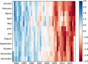
Figure 1. Anomalies in monthly sea-ice extent from November 1978 through July 2018. The colors indicate how many standard deviations sea-ice extent in a given month was above or below the mean sea-ice extent of the reference period 1981–2010.
Download figure:
Standard image High-resolution imageThe regions for which these anomalous ice losses occur are different for summer and winter (figure 2 and table 2). Summer ice losses have dominated the perennial ice cover, particularly in the Beaufort, Chukchi and East Siberian seas. These regions, with large ice coverage during winter but strong negative trends in summer, have been defined to be in 'summer mode' by Onarheim et al (2018). They evaluated SIC trends through December 2016 and found the largest sea ice reductions in terms of contribution to the total summer ice loss come from the East Siberian Sea (22%), followed by the Chukchi Sea (17%), the Beaufort Sea (16%), the Laptev Sea (14%) and then the Kara Sea (9%). Through 2018 we find the relative contributions have changed somewhat, with the East Siberian Sea continuing to lead the way (27%), followed closely by the Beaufort and Chukchi seas (16% and 15%, respectively), the Laptev (13%) and the Kara Sea (9%). In terms of explaining inter-annual variance in the September SIE since 1979, these six regions of the Arctic Ocean explain the majority (89%) of the inter-annual variance in total September SIE since 1979, with the Central Arctic and the Canadian Archipelago contributing the rest (Onarheim et al 2018). Finally, it is worth noting that relative to the average sea-ice coverage during the first decade of the satellite record (1979–1989), the Chukchi Sea, the Kara Sea, and the Hudson Bay have lost between 90% and 100 % of their September sea ice, while the Laptev and East Siberian Seas have lost between 80% and 90 % (see table 2).
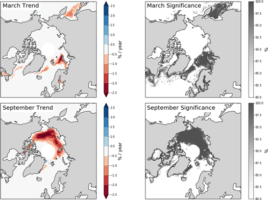
Figure 2. Sea ice concentration trends in percent concentration per decade during March (1979–2018) and September (1979–2017). Statistical significance of trends shown on right hand side.
Download figure:
Standard image High-resolution imageTable 2. Total loss or gain of sea ice extent and the corresponding linear trend over the period January 1979 through April 2018 (in km2) and % ice loss relative to 1979–1989. Total loss is calculated as the trend multiplied by the total number of years. Winter-mode regions are shaded in gray. Trends statistically significant at 90% and 95% confidence are marked by + and ++, respectively.
| March | September | |||||
|---|---|---|---|---|---|---|
| Region | Total ice loss (km2) | Relative loss (%) | Linear trend (km2 yr−1) | Total ice loss (km2) | Relative loss (%) | Linear trend (km2 yr−1) |
| Winter Mode Regions | ||||||
| Sea of Okhotsk and Japan | −358 300 | −28.8 | −8957++ | — | — | — |
| Bering Sea | −58 984 | −8.1 | −1475 | — | — | — |
| Gulf of St. Lawrence | −89 698 | −42.5 | −2242+ | — | — | — |
| Baffin Bay/Davis Strait/Labrador Sea | −222 441 | −15.7 | −5561+ | −32 171 | −50.0 | −825+ |
| Greenland Sea | −357 909 | −36.9 | −8947++ | −143 177 | −40.4 | −3671++ |
| Barents Sea | −453 442 | −47.2 | −11 336++ | −55 310 | −88.9 | −1418+ |
| Summer mode regions | ||||||
| Kara Sea | −14 371 | −1.6 | −359++ | −290 918 | −97.5 | −7459++ |
| Laptev Sea | 0 | 0 | 0 | −410 456 | −82.7 | −10 755++ |
| East Siberian Sea | 0 | 0 | 0 | −866 933 | −83.8 | −22 229++ |
| Chukchi Sea | 0 | 0 | 0 | −503 630 | −100 | −12 914++ |
| Beaufort Sea | 0 | 0 | 0 | −506 960 | −68.3 | −12 999++ |
| Canadian Archipelago | +10 | 0 | +0.2 | −149 819 | −32.9 | −3842++ |
| Central Arctic Ocean | −19 576 | −0.6 | −489 | −240 633 | −7.6 | −6170++ |
| Hudson Bay | 0 | 0 | 0 | −40 890 | −93.6 | −1046++ |
| Total | −1.687 106 | −10.6 | −42 181++ | −3.252 106 | −45.2 | −83 336++ |
During winter, the Arctic Ocean remains ice-covered and thus changes in winter are naturally limited to the seasonal seas. These seas with no sea ice during summer, and thus largest negative trends during winter have been defined to be in 'winter mode' by Onharheim et al (2018). They showed that the Barents Sea and Sea of Okhotsk show the largest overall reductions, each contributing 27% to the March SIE trend (Onarheim et al 2018), with the East Greenland Sea (23%) and Baffin Bay/Davis Strait/Gulf of St. Lawrence (22%) contributing the rest. However, updating trends through March 2018 shows that the East Greenland Sea and the Sea of Okhotsk now have similar trends, both contributing about 22% to the overall March SIE trend. Furthermore, these regions together explain 81% of the inter-annual variance in March SIE over the satellite data record (Onarheim et al 2018). Compared to ice conditions during the 1979–1989 time-period, the Barents Sea and the Gulf of St. Lawrence have lost about half their winter sea ice, while the Sea of Okhotsk and the Greenland Sea have lost roughly a third of their initial winter sea-ice cover (see table 2).
Continued warming may result in regions changing from a summer to a winter mode as the region starts to lose its summer sea ice. In this framework, the Kara Sea is currently in a transition from a summer to a winter mode as it has largely lost all of its summer sea ice cover in recent years, and winter trends east of Novaya Zemlya have turned slightly negative (see figure 2 and table 1). The fact that more and more regions enter the winter mode contributes to the record winter ice loss observed in the recent past.
How do changes in the melt season influence these winter and summer mode regions? Onarheim et al (2018) suggested these modes are strongly linked to the timing of melt onset and autumn freeze-up, with larger melt onset trends in the summer mode regions and larger freeze-up trends in the winter mode regions. This was based on an assessment of SIC trends rather than melt onset or freeze-up. Here we update the previously reported melt onset and freeze-up trends from Stroeve et al (2014a) using the Markus et al (2009) algorithm (figure 3). Melt onset trends are largest within the Barents and Kara seas, as well as Baffin Bay and the East Greenland Sea: regional averages are −8.2, −5.1, −6.6 and −7.1 days dec−1, respectively. The trends have slightly increased compared to those through 2013 (Stroeve et al 2014a). Hudson Bay also exhibits mostly negative trends (regional average of −3.6 days dec−1). Elsewhere, trends are mostly on the order of 2 to 3 days earlier per decade. Thus, in contrast to Onarheim et al (2018), we find melt onset trends are largest in regions which have little to no summer sea ice. However, since earlier melt onset leads to earlier development of open water and enhancement of the ice-albedo feedback, early melt onset within winter-mode regions helps to drive SIC reductions within the summer mode regions.

Figure 3. Trends in melt onset (upper-left) and freeze-up (upper-right) from 1979 through 2017 relative to 1981 to 2010 given in days per decade together with melt onset and freeze-up anomalies in 2016 (lower-left and lower-right, respectively).
Download figure:
Standard image High-resolution imageFor freeze-up, the largest trends are again in the Barents Sea (+14.5 days dec−1), but similar order of magnitude trends are also found in the Chukchi Sea (+14.3 days dec−1). In the Chukchi Sea, this large positive trend is dominated by later freeze-up in the northern and coastal regions, whereas freeze-up occurs near average in the southern Chukchi Sea. Other regions with trends more than 10 days per decade are found in the Kara and East Siberian seas (+10.4 and +11.6 days dec−1, respectively). Trends in the winter mode regions (besides the Barents Sea), are smaller and range from +7 to +8 days per decade, yet all trends reported here are larger than those previously found through 2013 (Stroeve et al 2014a), highlighting continued lengthening of the melt season in recent years.
It is interesting to consider these freeze-up and melt onset changes in the context of the particularly anomalously low sea ice conditions from January 2016 through April 2017, the period with 16 consecutive months of SIE more than 2σ below average. Melt onset in 2016 was the earliest recorded in the satellite data record within the Kara and Bering seas (18.7 and 16.4 days earlier than the 1981–2010 mean, respectively), and more than a month earlier in the Barents Sea (31.2 days earlier). In the southern Beaufort Sea, melt onset was also more than a month earlier than average and open water developed by the end of April. Thus, record low pan-Arctic ice conditions at the start of the 2016 melt season (e.g. April through May) were largely a result of early melt and ice retreat in the Barents, Kara, Bering and southern Beaufort seas. On the other hand, freeze-up in 2016 was the latest recorded in the satellite data record within the Barents and Kara seas, (65.1 and 39.6 days later than the 1981–2010 mean, respectively), and was also 25 to 35 days later than average in the Beaufort, Chukchi and E. Siberian seas. Overall, on a pan-Arctic scale, freeze-up over winter 2016/2017 was 17 days later than average, leading to new record low SIEs from November 2016 through March 2017.
3.2. Ice age and ice thickness
Since reductions in the age of the sea ice largely drive the observed sea-ice thickness changes (Maslanik et al 2007, Tschudi et al 2016a), we start with an update of ice age changes through April 2018 (figure 4). In stark contrast to conditions in 1984, there nowadays is virtually no perennial ice within the Chukchi and East Siberian Seas, and the Beaufort Sea consists primarily of a mixture of first-year and second-year ice. A tongue of second- and third-year ice stretches from the central Arctic towards the New Siberian Islands in 2018, and a considerable amount of second-year ice is also found near Sevemaya Zemlya.

Figure 4. Ice age during week 16 (last week of April) in 1984(a) and 2018 (b) (adapted from the National Snow and Ice Data Center (NSIDC)), and time series of percent of total extent of different age classes (c) as averaged over the Arctic Ocean Domain (insert). Note the data for 2018 is preliminary data courtesy M Tschudi (University of Colorado).
Download figure:
Standard image High-resolution imageOverall, the proportion of the Arctic Ocean Domain (see figure 4(d)) consisting of perennial ice in April declined from 59% in 1984 to 28% in 2018. The least amount of perennial ice in winter occurred in 2013 (24%), following the 2012 September minimum. While 2018 shows slightly more overall perennial ice than the year before, the amount of perennial ice with an age of 5 years or more was at a minimum (1.9%). For comparison, in 1984 about 28% of the Arctic basin consisted of ice with an age of 5 years or more. The loss of this oldest ice is arguably the most striking change in the sea ice cover within the Arctic Ocean Domain. The proportion of 4 year old ice has also seen a significant decline, dropping from 8.3% of the Arctic Ocean Domain to as low as 1.4% in 2011. Overall, the rate of decline of the 4 year old ice is −27.8% dec−1 compared to −50.0% dec−1 for the 5+ age class. This has been compensated by an increase in first-year ice at a rate of 16.3% dec−1 and in 2nd year ice at a rate of 3.3% dec−1.
The long-term shift from an old, thick perennial ice cover is reflected in the overall reductions in ice thickness simulated by PIOMAS. In figure 5 we show the April mean PIOMAS ice thickness from 1979 to 2017 for the entire Arctic region over which CryoSat-2 provides estimates of ice thickness (see Stroeve et al 2018 for the CryoSat-2 April mask region). PIOMAS results indicate that the Arctic Ocean mean ice thickness has declined by 28 cm dec−1, or 40% since 1979. For the CryoSat-2 period from 2010 onwards, ice-thickness estimates based on CryoSat-2 retrievals from CPOM, NASA and AWI span the range of PIOMAS-simulated mean thickness, with CPOM generally estimating slightly thicker ice than the other two CryoSat-2 products until April 2017, when the NASA product shows a distinct thickening compared to the previous year.

Figure 5. Mean April sea ice thickness for the Arctic Ocean from PIOMAS and three different data providers for CryoSat-2 (CPOM, AWI and NASA). See Stroeve et al (2018) figure 1(d) for the region used to calculate the mean thickness over.
Download figure:
Standard image High-resolution imageIn regards to winters 2015/2016 and 2016/2017, Stroeve et al (2018) previously evaluated the spatial patterns of sea ice thickness anomalies from these three CryoSat-2 thickness products and found general consistency in the direction of thickness anomalies from 2011 to 2017, even if absolute magnitudes differed. None of the CryoSat-2 thickness products suggested 2016 or 2017 were particularly anomalous compared to other years in the CryoSat-2 data record: instead the thinnest April ice cover appeared to occur in 2013. PIOMAS-simulated ice thickness estimates on the other hand suggest April 2017 was the thinnest. It remains unclear which of these results is more reliable: on the one hand, PIOMAS provides simulation results that are unconstrained by retrievals of sea-ice thickness. On the other hand, PIOMAS includes inter-annually varying snow fall, which, as indicated, the different CryoSat-2 estimates do not. Their short-term trends will hence always be biased if snow coverage departs from the long-term snow climatology that these algorithms employ. Nevertheless, the combination of ice age data, PIOMAS simulations and sea-ice thickness estimates based on CryoSat-2 retrievals suggest that the overall thickness of the Arctic Ocean has decreased significantly over the last 40 years, dropping to a mean value of approximately 2 m at the end of winter.
3.3. Change in tendency for rapid ice growth (RIGE) and rapid ice loss events (RILEs)
As the ice cover thins, the same amount of heat input can cause larger expanses of open water (e.g., Holland et al 2006, Maslanik 2007, Notz 2009). To more robustly assess if this has caused an increase in RILEs during summer, we examined the change in Arctic SIE over all 7 day long periods from November 1978 until today (figure 6). We define two different thresholds for RILEs, namely the loss of at least 800 000 (blue) or of at least 1 million km2 (red) of SIE within 7 d. We find that for both thresholds, the frequency of RILEs has substantially increased since 2005. Indeed, the first RILE with an ice loss of more than 1 million km2 only occurred in early July 2007, with similar events in early July 2014 and 2015. In 2012, the great cyclone during August resulted in a little less than 900 000 km2 of ice loss over a 7 day period. The largest amount of ice loss during any single week-long period occurred in early July 2007, with a total ice loss of nearly 1.2 million km2.

Figure 6. Total sea ice extent change during 7 day long periods. Absolute changes of sea ice extent of more than 800 000 km2 within a week are shown in blue, while absolute changes of more than 1 million km2 are shown in red.
Download figure:
Standard image High-resolution imageThe existing data also allows us to examine the probability for RIGEs in winter, which might have become more likely as larger and larger amounts of open water allow for the potential of rapid freeze-up. Again, evaluating the probability for RIGEs using the two different thresholds, we find a greater tendency for rapid ice growth in more recent years (figure 6). The single largest ice growth event, however, has so far occurred already in October 1995, amounting to 1.5 million km2. While most RIGEs occur during October, some years also witness RIGEs towards the end of September earlier in the data record (e.g. 1987, 1990, 1993, 1998, 2002), as well as later in the season such as November (e.g. 1989, 1992, 1995, 1997, 2004, 2006, 2014, 2015, 2016) and December (e.g. 2006, 2016). The extension of RIGEs later in the season is in agreement with later autumn freeze-up trends. Thus, while there is relatively rapid freeze-up as air temperatures drop, increases in ocean mixed layer temperatures have delayed the freeze-up and increased the potential for rapid freeze-up events towards later in the year.
4. Drivers of observed changes
As with any other change in the climate system, the observed loss of Arctic sea ice can be explained by a combination of three distinct factors that govern the evolution of climate: first, changes in the external forcing from anthropogenic sources. Second, changes in the external forcing from natural drivers. And third, internal variability of the climate system.
Substantial research has been dedicated to attribute the observed changes to a combination of these three factors, with the overall consensus view now being that changes in anthropogenic forcing and internal variability are by far the most important drivers of the observed loss. These drivers do, however, not affect the sea ice directly, but instead they modify the atmospheric and oceanic forcing on the ice cover, which then in turn cause the sea-ice cover to shrink and thus serve to visualize the often invisible changes in the atmosphere and in the ocean.
In this section, we first summarize our understanding of the role of the three general climate drivers for the observed loss of Arctic sea ice. We then turn to a detailed discussion of the various pathways by which the atmosphere and the ocean deliver changes in these climate drivers to the surface, ultimately causing the observed loss of the Arctic sea-ice cover in all seasons.
4.1. External forcing and internal variability as drivers of sea ice loss
There are two ways in which the climate system can reduce the amount of sea ice within the Arctic Ocean: first by local melting within the Arctic Ocean, and second by export of sea ice through southward sea ice drift. As outlined in the following sections, a number of studies have found the local melting of sea ice to be by far the main contributor to the observed loss, and we hence need to identify the main driver for increased sea ice melting if we are to identify the main driver for the substantial sea ice loss in recent decades.
Obviously, rising air temperature is a prime suspect for driving increased sea ice melt. This is first based on the simple fact that ice melts faster the warmer it is, but is further made plausible by the very robust linear relationship between the long-term trend in the spatial coverage of Arctic sea ice and the long-term trend in global mean near-surface air temperature, both in model simulations and in the observational record (Gregory et al 2002, Winton 2011, Mahlstein and Knutti 2012, Ridley et al 2012, Li et al 2013, Stroeve and Notz 2015, Rosenblum and Eisenman 2016, 2017, Niederdrenk and Notz 2018). This then in turn suggests that the main driver for the observed global warming—namely increases in atmospheric CO2 concentration from anthropogenic emissions (IPCC 2013)—is also the main driver for the observed loss of Arctic sea ice.
This relationship was made explicit in a study by Notz and Stroeve (2016), who showed that the loss of Arctic sea ice is directly correlated with anthropogenic CO2 emissions, both in the observational record and in all CMIP5 model simulations. They presented a simple conceptual argument that showed that the correlation can directly be explained by first principles, thus suggesting that the correlation is indeed established through a causal relationship between CO2 emissions and Arctic sea ice loss. Their argument can also explain the linear relationship between global-mean temperature and Arctic sea ice loss.
The linear relationship between Arctic sea-ice coverage and global mean temperature identified in earlier studies does not only hold in summer, but can be used to examine sea ice sensitivity for every single month. For example, Niederdrenk and Notz (2018) derive from observational records that in the long term, 3.3–4 million km2 of September Arctic sea ice are lost per °C of annual mean global warming, while the sensitivity in March is around 1.6 million km2 of sea ice loss per °C of annual mean global warming.
This year-round linear relationship between sea ice coverage and global warming goes along with a year-round linear relationship between Arctic sea ice coverage and anthropogenic CO2 emissions throughout the observational period (figure 7). For individual months, we estimate an ice loss per ton of anthropogenic CO2 emissions of slightly above 1 m2 during winter, and more than 3 m2 throughout summer. The comparably slow retreat during winter might at least in part be related to geographic muting. This term describes the fact that the outer winter ice edge is much shorter than the outer summer ice edge because the winter ice edge is usually interrupted by the large landmasses of Eurasia, Canada, Alaska and Greenland (compare Eisenman 2010). This suggests that the sensitivity of the winter sea-ice cover might be increasing in the future. Hence, any extrapolation of past winter sensitivities into the future are likely underestimating the future evolution of the winter sea-ice cover.
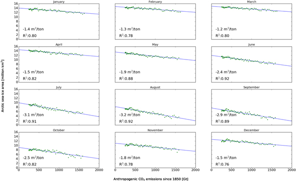
Figure 7. Relationship between observed Arctic sea ice area (y-axis) and total anthropogenic CO2 emissions (x-axis) for each month of the year for the period 1953 until 2017. The numbers in each subpanel denote the loss of sea ice area per ton of CO2 emissions and the R2 value of the linear fit.
Download figure:
Standard image High-resolution imageIn addition to this clear, primarily anthropogenic impact on the long-term evolution of Arctic sea ice, internal variability can substantially amplify or dampen this loss, in particular on shorter time scales (e.g. Swart et al 2015, Notz 2015, Jahn et al 2016). It is difficult however, to robustly assess the contribution of internal variability to the observed loss, as this is only possible with climate models, which differ widely in their estimated magnitude of internal variability of the Arctic sea-ice cover (e.g., Olonscheck and Notz 2017). Because of the relative shortness of robust observational records and because of their large externally forced trends, the 'correct' internal variability can currently not be established. Based on the available studies, it seems nevertheless likely that a substantial fraction of the observed rapid loss in the early 21st century has been caused by internal variability. For example, based on an analysis of changes in atmospheric circulation, Ding et al (2017) estimate that about 40% of the observed sea ice loss has been driven by internal variability (see detailed discussion in section 4.3). Also, Notz (2017) provides evidence that the rapid loss of Arctic sea ice in the early 21st century was amplified by internal variability: 10 year long trends of Arctic sea ice evolution closely follow the average 10 year long-term trend of hundred members of a large ensemble simulation with the ESM MPI-ESM for most of the satellite record (implying a negligible impact of internal variability) but are at the extreme end of the ensemble spread of individual 10 year long-term trends early in the 21st century (implying a very large impact of internal variability). These studies hence suggest the characterization of the rapid loss of Arctic sea ice as an extreme event, caused by a combination of a long-term anthropogenically driven sea ice loss, amplified by short-term internal variability.
The impact of natural changes in external forcing on the Arctic sea ice cover has been weak in recent decades. For example, only in large ensembles of simulations from the same model, the impact of occasional volcanic eruptions can be separated from the much larger internal variability of the Arctic sea-ice cover (e.g. Notz 2017). Rosenblum and Eisenman (2016) suggest that erroneously exaggerated volcanic forcing in CMIP5 simulations might be the main reason for why these simulations show a trend in Arctic sea ice in broad agreement with observations, yet Santer et al (2017) find the models' change in global mean surface temperature to volcanic eruptions to be fairly realistic.
4.2. Stability of the ice cover
In addition to changes in the external forcing and internal variability, a self-amplification of the ongoing ice-loss could in principle have contributed to the rapid ice loss in recent years. Such self-amplification is usually discussed in the context of so-called tipping points or nonlinear threshold, which are often defined as processes in the climate system that show substantial hysteresis in response to changed forcing.
The best known example for such possible hysteresis behavior is related to the ice-albedo feedback mechanism: a reduced ice cover in a given summer will cause increased absorption of solar radiation by the ocean, contributing to further reductions in the ice cover. Such positive feedback loop can cause the irreversible loss of Arctic sea ice in idealized studies based for example on energy-balance models (see review by North 1984), and have hence been suggested to possibly be relevant also for the real world.
However, an analysis of the existing observational record and a substantial number of respective modeling studies with complex ESMs all agree that such a 'tipping point' does not exist for the loss of Arctic summer sea ice. For example, Notz and Marotzke (2012) found a negative auto-correlation of the year-to-year changes in observed September SIE. Hence, whenever SIE was substantially reduced in a given summer, the next summer usually showed some recovery of the ice cover. This was further supported by Serreze and Stroeve (2015). Such behavior suggests that the sea-ice cover is at least currently in a stable region of the phase space, as otherwise one would then expect that any year with a really low ice coverage should be followed by a year with an even lower ice coverage, driven by the ice-albedo feedback mechanism. As shown by Tietsche et al (2011), the contrasting behavior of the real ice cover can be explained by compensating negative feedbacks that stabilize the ice cover despite the amplifying ice-albedo feedback. The most important of these stabilizing feedbacks relates to the fact that during winter the ocean very effectively releases heat from those areas that became ice free during summer, thus over-compensating for any extreme ice loss in a preceding summer. Ice that is formed later in the season also carries a thinner snow cover and can hence grow more effectively during winter (e.g., Notz 2009). Stroeve et al (2018) suggest, however, that this stabilizing feedback mechanism is becoming weaker and weaker as Arctic winters become warmer and warmer. Increased winter cloud cover after summer sea ice loss as found by Liu et al 2012 also weakens the stabilizing feedback, as it reduces the loss of heat from the ocean surface.
The apparent mismatch of observations and complex model studies on the one hand, which both show no emergent tipping-point behavior of the ice loss, and studies with idealized models, which show tipping-point behavior, was resolved in a dedicated study by Wagner and Eisenman (2015). They were able to extend simplified models until their behavior agreed with more complex models. In doing so, they found that both spatial communication through meridional heat transport and the annual cycle in solar radiation are important for stabilizing the ice cover's response to changes in the external forcing.
For winter sea ice, the situation is different. Here, even complex ESMs show a sudden acceleration of the ice loss in response to a slow increase in the external forcing, and the eventual loss of winter sea ice occurs sometimes substantially faster than the preceding loss of summer sea ice. Bathiany et al (2016) explain this behavior by a simple geometric argument: The loss of summer sea ice proceeds comparably slowly, because the ice thickness distribution is rather broad and in a given summer, the thinnest ice disappears while thicker ice might stay behind. For the loss of winter sea ice, however, the distribution in ice thickness will be much narrower, as only first-year ice will be left behind. Once temperatures have risen enough to prevent ice formation during winter, the Arctic Ocean can rapidly change from an ocean largely ice covered in winter to an ocean that remains ice free throughout winter.
4.3. Atmospheric pathways
Having thus established that a combination of internal variability and anthropogenic forcing is largely responsible for the observed ice loss, the question naturally arises how specifically these drivers affect the Arctic sea ice cover. A study by Burgard and Notz (2017) has found that CMIP5 models disagree on whether the anomalous heating of the Arctic Ocean, and thus the loss of Arctic sea ice, primarily occurs through changes in vertical heat exchanges with the atmosphere (as is the case in 11 CMIP5 models), primarily through changes in meridional ocean heat flux (as is the case in 11 other CMIP5 models) or through a combination of both (as is the case in 4 CMIP5 models). This suggests that our understanding of how precisely the heat for the observed sea ice melt is provided to the sea ice is still surprisingly limited. This caveat should be kept in mind when assessing the robustness of studies that examine the detailed atmospheric and oceanic drivers of Arctic sea ice melt.
Focusing first on the atmosphere, changes in the sea-ice cover can occur through dynamical changes that drive ice export (e.g. Rigor et al 2002, Ogi and Wallace 2007, L'Heureux et al 2008, Wang et al 2009, Smedsrud et al 2017), thermodynamical influences (e.g. Kay et al 2008, Ding et al 2017), or a combination of both (Graversen et al 2006, Graversen and Burtu 2016). As an example for the combined acting of dynamic and thermodynamic forcing, winds that drive the sea ice away from shore are often warm, southerly winds that can enhance ice melt, such as observed during summer 2007 (Stroeve et al 2008).
Early studies examined the influence of the Arctic Oscillation (AO) during winter on the summer sea ice cover, finding that the predominantly positive phase of the AO in the late 1980s through mid-1990s decreased September sea ice coverage by increasing offshore ice advection off the coasts of Siberia (Rigor et al 2002, Zhang et al 2003). Rigor and Wallace (2004) showed that this phase was additionally linked to a reduction in the mean ice age and thus of average sea-ice thickness within the Arctic basin since. This was because the deepening of the low pressure over Iceland increased the export of old ice through Fram Strait. However, since the mid-1990s the AO has oscillated between positive and negative phases and there is no clear trend in sea level pressure over the Arctic in winter (e.g. DJF SLP trends in figure 8 are not statistically significant at the 95% confidence level); yet the summer ice cover has continued to decline. More recently Williams et al (2016) found winter preconditioning continues to play a large role in September sea ice variability. In particular, winter ice export out of Fram Strait is strongly correlated to the anomaly of the following September SIE, allowing for the possibility of forecasting sea ice conditions in September several months in advance. Smedsrud et al (2017) also found a moderate influence of Fram Strait ice export on the following September SIE, explaining roughly 26% of the variance from 1979 to 2014. Yet, while the amount of ice exported through Fram Strait has increased over the satellite data, the increased ice export might instead be linked to the fact that that a thinner ice pack is more mobile (e.g. Rampal et al 2009, Olason and Notz 2014).

Figure 8. Seasonal sea level pressure trends from 1979 to 2017 using CFSRv2 Reanalysis. Regions with statistically significant trends at 95% confidence are highlighted in green.
Download figure:
Standard image High-resolution imageOn the other hand, changes in atmospheric circulation have led to anomalous winter warming over the Arctic Ocean in recent years (e.g. Cullather et al 2016, Graham et al 2017). Graham et al (2017) evaluated changes in frequency and duration of winter warming events since 1979, finding a significant trend towards increased frequency and duration of winter cyclones. These storms bring moist, warm air into the central Arctic Ocean, and are responsible for air temperatures rising above 0 °C at the pole in the middle of winter during each of the last 3 years. These events have contributed to very large reductions in total freezing degree days in winter (figure 9).
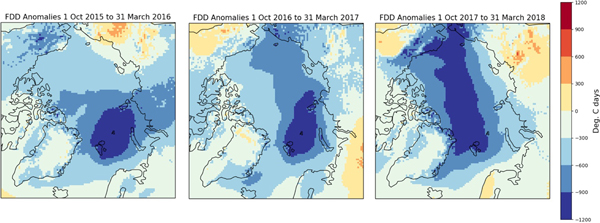
Figure 9. Freezing degree day anomalies during winter 2015/2016 (left), winter 2016/2017 (middle) and winter 2017/2018 (right). Freezing degree day anomalies are computed using CFSRv2. Anomalies are computed relative to 1981–2010.
Download figure:
Standard image High-resolution imageSeveral recent studies have evaluated how these warm winters may be impacting winter ice growth (Boisvert et al 2016, Ricker et al 2017, Stroeve et al 2018). This has been accomplished through evaluations of changes in SIC, surface energy balance and PIOMAS thickness (Boisvert et al 2016), through estimating ice growth through a simple relationship between freezing degree days and thermodynamic ice growth and comparing with CryoSat-2 and SMOS thickness estimates (Ricker et al 2017), or through combining CryoSat-2 observations with a sea ice model (Stroeve et al 2018). However, the challenge in accurately assessing the impact of observed winter warming events on thermodynamic ice growth using satellite observations remains the incomplete knowledge of snow depth variability. Models on the other hand can only accurately simulate thermodynamic ice growth if the prescribed atmospheric and oceanic forcing are realistic, which is not always the case. Notwithstanding these uncertainties, all studies have shown that the recent winter warming events are influencing the ice cover and have contributed to the substantially reduced winter ice extent in recent years.
Turning to the summer season, many more studies have addressed summer circulation patterns and their role in driving continued summer ice loss. These studies have generally addressed the influence of various atmospheric indices, such as the Arctic Dipole anomaly pattern (e.g. Wu et al 2006, Wang et al 2009, Overland et al 2012), the Arctic Rapid change Pattern represented by intensification of the Siberian High and weakening of the Aleutian low (Zhang et al 2008), the influence of the Pacific North American pattern (L'Heureux et al 2008), or the importance of cyclonic and anticyclone summers (Screen et al 2011). However, defining atmospheric circulation patterns by indices and their influence on the sea-ice cover misses other important contributions to sea ice variability, as the specific location of pressure anomalies is important, too (Serreze et al 2016a, Ding et al 2017). Ding et al (2017) provides the most recent characterization of the role of atmospheric variability on the observed summer sea ice, showing that trends in atmospheric circulation patterns in summer (i.e. a more anticyclonic circulation pattern) have increased the downwelling longwave radiation towards the surface as a result of a warmer and moister atmosphere. They further suggest that these circulation changes dominate summer ice variability rather than feedbacks from a changing sea ice cover.
It is clear that the anticyclonic pattern during summer has become more prominent in recent years (Moore 2012, Wu et al 2014, Serreze et al 2016a). Positive SLP trends are found over the central Arctic Ocean and Greenland, coupled with low SLP over Eurasia and North America (figure 8). This pattern favors more ice melt under the higher SLP and clearer skies, while also enhancing ice advection polewards between the pressure gradients and bringing warm, southerly air over the central Arctic.
In addition to atmospheric circulation changes in summer and winter, related changes in spring are also important. For example, numerous studies have shown the importance of the ice-albedo feedback for sea-ice evolution throughout summer, including the importance of the timing of melt onset and sea ice retreat on the amount of open water that develops in summer (Perovich et al 2008, Stroeve et al 2012a, 2014a, 2016, , Schroeder et al 2014). Circulation patterns that advect warm, moist air into the Arctic appear essential in initiating melt onset (Mortin et al 2016). Negative SLP trends in springtime are statistically significant in the Barents Sea (figure 8), which also is the region with the largest melt onset trends (figure 3). The trends in SLP imply additional warm air advection over the Barents Sea from the south, hence contributing to the earlier melting. During autumn, statistically significant negative SLP trends dominate the East Siberian, Chukchi and Beaufort seas, as well as the Canadian Arctic Archipelago (figure 8), yet there is a large amount of year-to-year variability (not shown). These negative autumn SLP trends are likely a direct response to the observed sea ice loss (e.g. Deser et al 2016, Blackport and Kushner 2017).
Finally, it is worth discussing how the role of summer cyclones on the sea ice cover may be changing. In the past, cyclonic summers resulted in overall larger SIE (e.g. Screen et al 2011), by spreading the ice cover over a larger area. However, as the ice cover has thinned, this relationship appears to have changed, as suggested by Serreze et al (2003) to explain the 2002 September minimum, and by Zhang et al (2013) to explain the 2012 minimum. The key is how much open water is fostered by sea ice divergence during a cyclonic event, how much the ice-albedo feedback is enhanced in these open water areas, how much sea ice-wave interaction occurs, and whether or not the divergent ice motion pushes ice into warmer ocean waters where it can melt out. The reduction in total SIA increases with cyclone intensity.
4.4. Oceanic pathways
The term Atlantification first found its way into scientific literature in 2012 in a study by Årthun et al (2012). In that study, Atlantification referred to the warming of the Barents Sea surface layer from increased Atlantic heat inflow, both from a strengthening and warming of the inflow. The penetration of warm Atlantic heat input began with the great thermal anomaly in Fram Strait in 1989, with temperatures 1 °C warmer than in the 1970s (e.g. Carmack et al 1995). This heat anomaly progressed through the Eurasian basin, arriving in the Laptev Sea in 1993, and eventually reached the Beaufort Sea in 2003. Another large pulse of warm water occurred in the 2000s, peaking in 2007 (Polyakov et al 2013), with an anomaly of 0.24 °C relative to the 1990s. This ocean warming largely explains the observed Barents Sea winter ice variability (Årthun et al 2012, Smedsrud et al 2013), and provides a useful predictor for the annual mean sea-ice cover in the Barents Sea (Onarheim et al 2015). The Barents Sea region has also been identified as key for explaining model differences between oceanic and atmospheric pathways of energy transfer to the central Arctic Ocean (Burgard and Notz 2017). Given this relationship, others have gone further to suggest that some recovery of the sea-ice cover may be possible if the spin-down of the thermohaline circulation continues (Yeager et al 2015).
While a clear fingerprint of oceanic heat on the winter sea ice in the Barents Sea has been identified, it is unclear how this warming may have impacted the ice cover elsewhere as this warm water has traditionally been separated from melting sea ice because of the strong halocline. Polyakov et al (2017) showed that this halocline has weakened, leading to increased winter ventilation and subsequently reduced winter ice formation. The Atlantification of the eastern Eurasian Basin may therefore provide an additional factor behind sea ice reductions in that region, perhaps on the same order of magnitude as atmospheric thermodynamic forcing.
On the Pacific side of the Arctic, Woodgate et al (2010) examined the role of Pacific waters on sea ice retreat in summer 2007. Mooring observations of Bering Strait ocean heat fluxes showed anomalous heat flux in 2007, more than twice the 2001 heat flux (3–6 1020 J yr−1), enough heat to melt 1/3rd of the annual Arctic sea ice cover (or 1–2 106 km2 of 1 m thick ice). However, the timing of this heat will largely determine its overall influence. If the oceanic heat inflow happens early enough to lead to early ice retreat, the ice-albedo feedback is further enhanced and more ice can melt. In fact, the timing of ice retreat within the Chukchi Sea is most strongly related to oceanic heat inflow through the Bering Strait (Serreze et al 2016b). Early ice retreat in turn leads to a longer period over which the ocean mixed layer can warm, which in turn will delay the autumn freeze-up (Stroeve et al 2016), though this relationship changes in the Chukchi Sea where ocean advection plays a larger role (Steele and Dickinson 2016). Including both the timing of ice retreat (which influences ocean mixed layer temperatures) and Bering Strait heat inflow in a predictive model was found to explain 67% of the variance in the timing of when the ice returns (Serreze et al 2016b).
Timmermans et al (2017) investigated the fate of the surface water in the Chukchi Sea warmed by solar radiation. Warming of summer sea surface temperatures in the Chukchi Sea by 0.5 °C since 1982 (Timmermans and Proshutinsky 2016) has ventilated the Canada Basin halocline, doubling the ocean heat content in the Beaufort Gyre halocline over the last three decades. This is equivalent to about 0.8m of sea ice melt.
4.5. Other potential influences: role of freshwater discharge
Freshwater input into the Arctic Ocean is primarily provided through precipitation, sea ice melt and river discharge. Additional sources include Pacific water inflow, glacial/ice sheet melt, iceberg melt and groundwater. Over the last two decades, the amount of freshwater in the Arctic has increased. This is particularly evident in the Beaufort Gyre, which has accumulated an extra 5000 km3 of freshwater in the 2000s compared to the 1980s and 1990s (e.g. Haine et al 2015). Contributions from rivers, streams and groundwater discharge represents about 3900 ± 390 km3 yr−1. This estimate is based on information from river discharge observations (Shiklomanov 2010) and runoff estimated from atmospheric reanalysis (see Haine et al 2015).
A few studies have evaluated how this freshwater discharge from rivers has impacted the sea ice cover (e.g Ngiehm et al 2014, Dean et al 1994). One way is through adding extra heat to the coastal regions. The large Eurasian and North American rivers input warm freshwater (on average 15 °C) with a distinct seasonal cycle along the shallow shelf seas (e.g. Carmack et al 2016). Peak discharge occurs in June and this water is immediately available to melt ice, helping to break up the fast ice. River discharge also adds a large amount of chromophoric dissolved organic matter, which absorbs sunlight at short wavelengths (Griffin et al 2018), further warming the surface layers of the ocean and increasing ice melt. On the other hand, increased ice melt and freshwater input increases summer stratification, allowing for more heat to be trapped in the upper ocean, which in turn delays ice formation in autumn.
5. Implications
The retreat of sea ice in all seasons has already had profound impacts on the energy balance of the Arctic and has contributed to Arctic amplification, i.e. the faster warming in the Arctic compared to mid-latitudes, particularly during autumn and winter (e.g., Serreze et al 2009, Screen and Simmonds 2010, Pithan and Mauritsen 2014, Walsh 2014). However, sea ice loss is not the only factor behind observed winter warming, and other factors contribute at other times of year as well. One such factor is an increase in downwelling longwave radiation from greenhouse gases (Notz and Stroeve 2016), atmospheric moisture from local (e.g Serreze et al 2012, Boisvert and Stroeve 2015, Kim et al 2017) and remote sources (e.g. Graversen 2006, Zhang et al 2013, Mortin et al 2016, Woods and Caballero 2016), and increases in cloud cover (Kay and L'Ecuyer 2013, Jun et al 2016). Other factors include changes in oceanic heat content (Polyakov et al 2005, Walsh 2014, Ivanov et al 2016), enhanced poleward heat transport (e.g. Zhang et al 2008), and the phase of the Pacific Decadal Oscillation (PDO), which modulates how the sea-ice cover influences this warming (Screen and Francis 2016), such that some sea ice reduction years have a smaller influence on tropospheric warming than others.
The so-far more rapid ice loss during summer has changed the seasonality of the Arctic, such that the annual cycle of its sea-ice cover is becoming more comparable with the seasonality of the Antarctic (Haine and Martin 2017); or the Antarcticification of the Arctic. This change in seasonality of the sea ice and hence the Arctic climate system influences all aspects of the Arctic ecosystems (e.g. Symon et al 2004, Post et al 2013), including changes in vegetation (e.g. Xu et al 2013, Fauchald et al 2017), permafrost temperatures (e.g. Lawrence et al 2008); and the entire marine ecosystem (e.g. Wassmann et al 2011, Darnis et al 2012). With the melt season continuing to start earlier and lasting longer, one expects local warming over adjacent land areas to increase, which may increase terrestrial primary productivity by early greening of vegetation (Dutrieux et al 2012) as well as delaying soil freeze dates (Chapin et al 2008).
Less is known about how early retreat and late ice formation, in addition to a thinning ice cover may influence the marine food web. The sea ice matrix offers protected habitat for microbial life and together with phytoplankton forms the base of the Arctic marine food web, sustaining sea ice associated macrofaunal and part of the pelagic zooplankton (e.g. Kolbach et al 2016). The growth of algae and phytoplankton depend strongly on light availability, and thus as the sea ice seasonality changes and thick multiyear ice is replaced by thinner first-year ice, the amount of light available to the upper ocean increases, which may increase blooms. Too much light, however, can be harmful to Arctic algae, which usually are well adopted to the rather low-light conditions that have been the prevailing light conditions under the Arctic sea-ice cover. In addition, primary production is a complex interplay between light, nutrient availability and ocean stratification. A further challenge is how the human dimension will modify these influences. For example, the loss of sea ice will likely accelerate resource extractive industries and it increases accessibility of remote marine areas which could have negative consequences for many marine species.
While it is understood that changes happening within the Arctic do not stay there, it is less certain whether current Arctic warming is already driving an increase in storm frequency and extreme weather events across the mid-latitudes, including extreme heat and rainfall events, and more severe winters. The possibility of a link has driven an increased number of studies to examine linkages in more detail. A host of mechanisms and processes have been proposed and some consensus has emerged; namely that amplified Arctic warming, regardless of its driver, has increased geopotential height thickness (Francis and Vavrus 2012, Cvijanovic et al 2017), which in turn has weakened the thermal wind (Francis and Vavrus 2012, Walsh 2014, Pedersen et al 2016). It is not clear, however, how much these atmospheric changes have influenced the jet stream (Barnes 2013) or the influence on storm tracks and occurrence of blocking events (Zhang et al 2012, Barnes et al 2014, Barnes and Screen 2015). It is entirely possible that such a link exists, yet its manifestation in the real world is likely only of minor importance given the substantial year-to-year variability arising from internal variability of the climate system.
Part of the difficulty in assessing the contribution of Arctic sea ice loss to changes in weather conditions derives from the fact that different modeling studies give divergent results depending on the specific model set-up (e.g., Sun et al 2016, Screen et al 2018). Another key aspect is our still poor understanding on the two-way interactions between the tropospheric and stratospheric polar vortex.
The region considered most robust in terms of Arctic-mid-latitude linkages is during winter in the Kara and Barents Sea. This region has seen the largest reductions in winter ice cover (e.g. Onarheim and Årthun 2017), that in turn influence the exchange of turbulent heat fluxes between the ocean and the atmosphere, resulting in a northwestward expansion of the Siberian high (e.g. Mori et al 2014). Perturbation of the pressure over Siberia leads to a weakening of the stratospheric polar vortex through tropospheric-stratospheric coupling, providing a clear link between sea ice changes and winter cooling over Eurasia (e.g. Kim et al 2014, Kretschmer et al 2016, 2018). These links are robust in both observational and modeling studies.
However, it is important to remember that these changes do not happen in isolation from changes elsewhere on the planet. Modulation of the climate by tropical (e.g. El Nino/Southern Oscillation (ENSO), Madden Julian Oscillation (MJO)) and extratropical forcing (Atlantic Multidecadal Variability (AMV) and Pacific Decadal Oscillations (PDO)) also play a role. Thus, any Arctic and mid-latitude linkage may be strongly state-dependent, such that linkages are more favorable under one atmospheric wave pattern than another, and thus any link may be preconditioned by the state of the hemispheric background atmospheric flow (Overland et al 2016).
Finally, the loss of the summer sea ice cover opens up the potential for increased shipping activities, new fisheries and new locations for resource extraction. Regarding shipping, Smith and Stephenson (2013) find that the Northern Sea Route becomes navigable for both the RCP4.5 and the RCP8.5 emission scenarios by mid-century. While internal variability will continue to substantially affect the ease of transit from one year to the next, in terms of long-term planning the future emission pathways are the main source of uncertainty. For example, Melia et al (2016) find that by the end of the century, the possible shipping period reaches a duration of 4 to 8 months in the high emission RCP8.5 scenario, while it is just about half that long for the low-emission scenario RCP2.6. Other estimates project 5 months of ice free conditions along the Northern Sea Route by the end of this century under RCP8.5, using both SIC and ice thickness constraints (Bensassi et al 2015). In practice, the future use of these shipping routes will substantially depend on the economic and geopolitical boundary conditions (e.g., Ho 2010, Schøyen and Bråthen 2011, Bensassi et al 2015) and on the type of ship used for the transit (Smith and Stephenson 2013, Melia et al 2016).
6. Conclusions
Through novel analysis and a review of recent studies, we have examined the ongoing ice loss of Arctic sea ice across all seasons. We have established the following key results:
- 1.With respect to the 1981–2010 reference period, relative ice loss has been more significant during autumn, winter and spring the last two years than during summer (figure 1).
- 2.
- 3.The thinning of the ice cover and the overall warming of the Arctic have increased the likelihood of rapid ice-loss events during summer in recent years (figure 6). On the other hand, the larger expanses of open water have similarly increased the likelihood of rapid ice-growth events during autumn.
- 4.The increasing relative loss of winter sea ice is in part related to the fact that more and more regions of the Arctic Ocean completely lose their sea-ice cover during summer (figure 2). This limits the potential for a further acceleration of summer sea ice loss, and causes accelerating sea ice loss during winter.
- 5.Accelerated sea ice loss during all months of the year is additionally driven by a lengthening of the melt season. As assessed for the Arctic as a whole through April 2018, melt onset is occurring 3 days earlier per decade, and freeze-up is happening 7 days later per decade (figure 3). Over the 40 year long satellite record, this amounts to a 12 day earlier melt onset and a 28 day later freeze-up.
- 6.
- 7.The primary cause of the ongoing changes in all months are anthropogenic CO2 emissions, with a clear linear relationship between sea ice loss and cumulative anthropogenic CO2 emissions in all months (figure 7). The sensitivity ranges from an ice loss per ton of anthropogenic CO2 emissions of slightly above 1 m2 during winter, to more than 3 m2 throughout summer.
This last finding possibly has the largest policy implications of all our results: based on the study of Notz and Stroeve (2016), it allows us to estimate the future seasonality of the Arctic Ocean directly from the observational record (figure 10). Extrapolating the linear relationships into the future, we find that the Arctic Ocean completely loses its ice cover throughout August and September for an additional roughly 800 ± 300 Gt of anthropogenic CO2 emissions. For an additional 1400 ± 300 Gt of anthropogenic CO2 emissions, we estimate the Arctic to become sea-ice free from July throughout October (see Notz and Stroeve 2018 for details on these estimates, in particular regarding the uncertainty arising from internal variability).
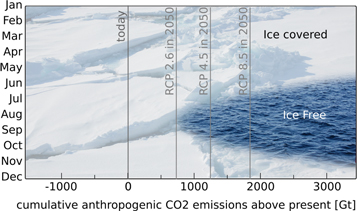
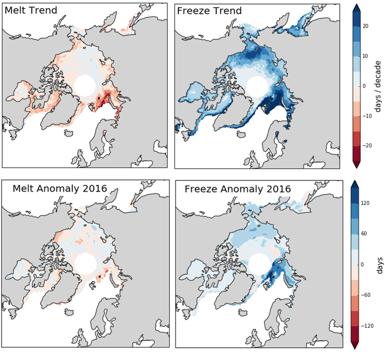
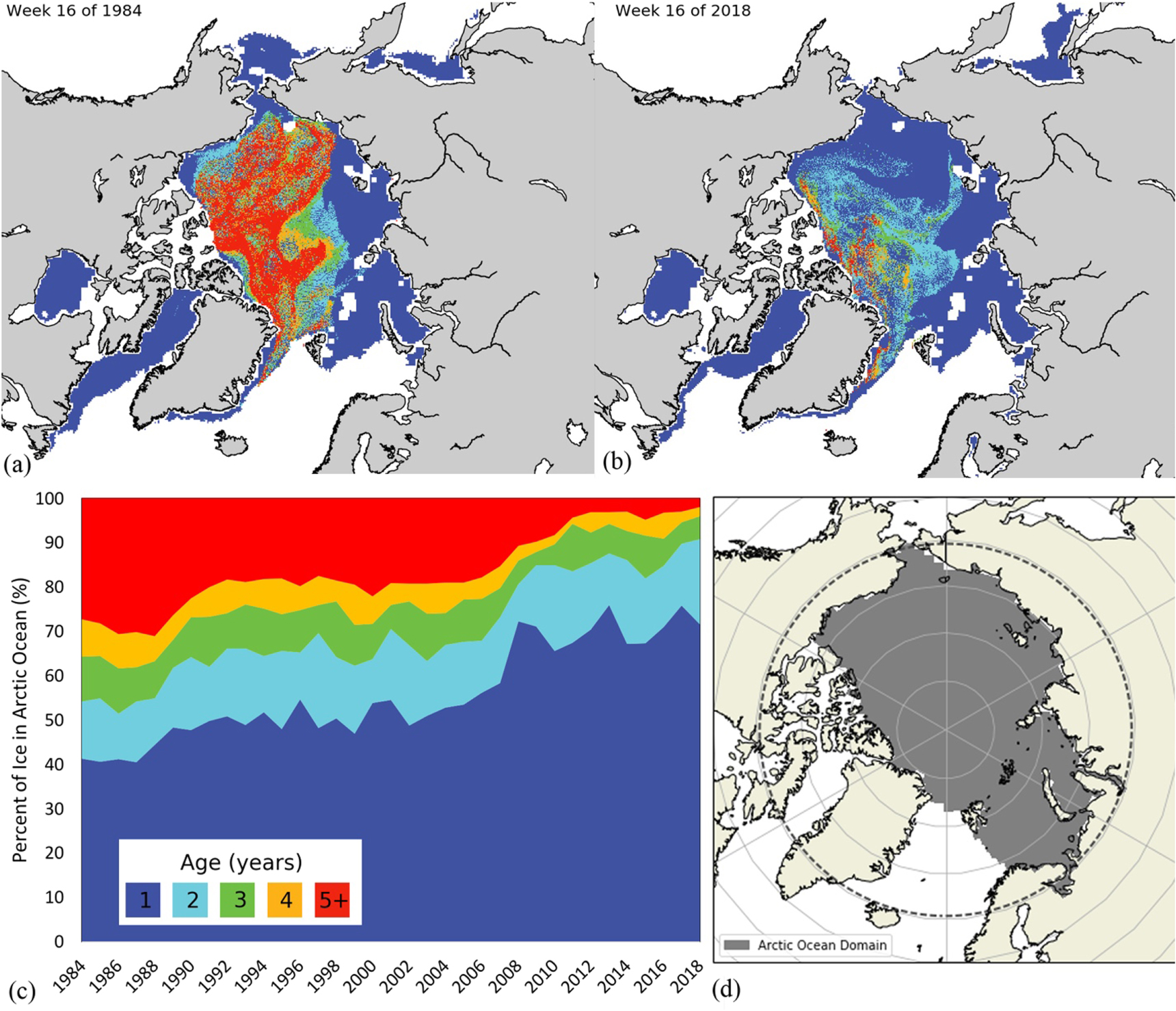
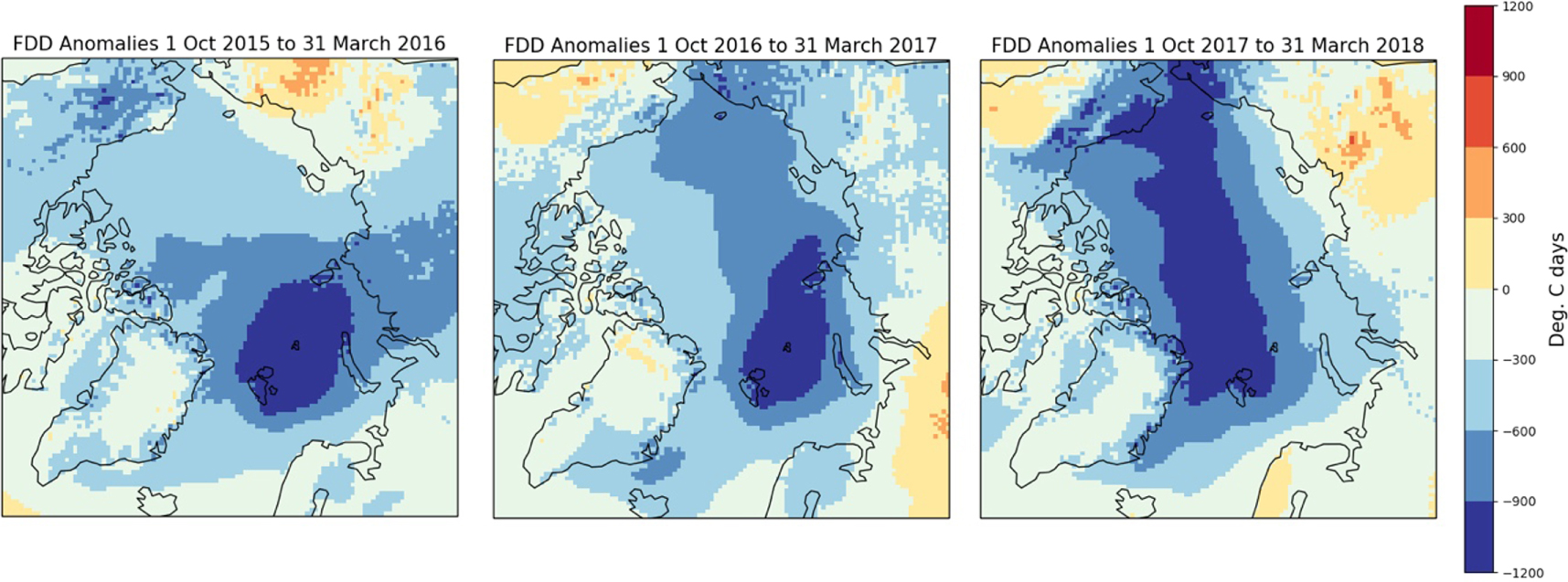
Figure 10. Estimated seasonality of the Arctic sea-ice cover as a function of anthopogenic CO2 emissions. The estimate is based on a linear extrapolation of the sensitivities shown in figure 7 until the ice cover reaches zero for a given month. Today's total CO2 emissions are around 1600 Gt since 1850, increasing at a rate of about 40 Gt per year. The shaded band around the ice-free region represents uncertainty arising from internal variability and observational uncertainty. Cumulative CO2 emissions relative to today for the different CMIP5 RCPs are included for reference.
Download figure:
Standard image High-resolution image
Given today's emission rate of about 40 Gt CO2 per year, the time window is closing very rapidly to preserve Arctic sea-ice cover all year round.
Acknowledgments
We are grateful to three anonymous referees for their valuable and insightful feedback on an earlier version of this manuscript. This work was in part funded under NASA grant NNX16AJ92G (Stroeve). Sea ice concentration data were obtained from NSIDC Sea Ice Index (http://nsidc.org/data/seaice_index). We are grateful to Jeff Miller at NASA GSFC for providing updated melt onset and freeze-up data, Andy Barrett at NSIDC for data and figure processing, Michel Tsamados, David Schroeder Andy Ridout at CPOM for CPOM CryoSat-2 data. AWI CryoSat-2 data is funded by the German Ministry of Economics Affairs and Energy (grant: 50EE1008) and data from November 2010 to April 2017 obtained from http://meereisportal.de (grant: REKLIM-2013–04). NASA CryoSat-2 data provided courtesy of Nathan Kurtz. NCEP CFSv2 data available from https://rda.ucar.edu/datasets/ds094.0/.