


Abstract
Observations show a significant positive correlation between the Atlantic Multidecadal Oscillation (AMO) and the Indian Summer Monsoon (ISM) over the past 100 years. Whether this connection is intrinsic to the climate system or caused by external forcing remains unclear in view of the substantial existence of anthropogenic greenhouse gases and aerosols in observations. Two state-of-the-art climate models (GFDL-CM3 and HadGEM2-ES), the historical simulations (1850–2005) of which show positive correlations between the AMO and ISM, similar to observation, are used to address this question. A significant positive AMO-ISM correlation exists in the control simulations with fixed preindustrial forcing with HadGEM2-ES, but not with GFDL-CM3. An in-depth analysis illustrates that the positive correlation in the HadGEM2-ES control run is more reasonable, since it simulates a similar teleconnection of the AMO with the North Pacific to that in both observations and previous studies. In comparison, the GFDL-CM3 control run fails to simulate the teleconnection of the AMO with the North Pacific. The positive AMO-ISM correlation in the historical simulation in GFDL-CM3 may be attributable to the role of the external forcing, since it is so strong that the AMO signals are excited additionally in the North Pacific. This study suggests that the AMO-ISM connection is intrinsic to the climate system, and highlights the crucial role played by the North Pacific in bridging such a connection.
Export citation and abstract BibTeX RIS

Original content from this work may be used under the terms of the Creative Commons Attribution 3.0 licence. Any further distribution of this work must maintain attribution to the author(s) and the title of the work, journal citation and DOI.
1. Introduction
The Atlantic Multidecadal Oscillation (AMO), as the leading pattern of the multidecadal variation in sea surface temperatures (SSTs) in the North Atlantic, has been associated with regional climate variations over many parts of the globe on a multidecadal timescale (e.g. Delworth and Mann 2000, Sutton and Hodson 2005, 2007, Li and Bates 2007, Ting et al 2011, Wyatt et al 2012, Drinkwater et al 2014, Ruprich-Roberts et al 2017). The connection between the AMO and the Indian Summer Monsoon (ISM) has been extensively investigated (e.g. Zhang and Delworth 2005a, Goswami et al 2006, Lu et al 2006, Feng and Hu 2008, Li et al 2008, Wang et al 2009, Luo et al 2011, Krishnamurthy and Krishnamurthy 2016) as a result of the observed AMO-ISM linkages over the past 100 years and the profound impacts of the ISM on the societies and ecosystems of India. These previous modeling studies have suggested that the AMO modulates the variation of the ISM on multidecadal timescales via air–sea interactions and atmospheric teleconnections (e.g. Zhang and Delworth 2005b, Feng and Hu 2008, Li et al 2008, Luo et al 2011). However, most early studies aimed at addressing the AMO-ISM connection focused on either the industrial era (after 1860) (e.g. Lu et al 2006, Li et al 2008, Wang et al 2009, Luo et al 2017, Ruprich-Roberts et al 2017) or idealized cases (water hosing experiments) (e.g. Zhang and Delworth 2005b, Yu et al 2010).
Luo et al (2011) found a positive AMO-ISM correlation in a 600 year control simulation of the Bergen Climate Model, version 2. However, based on 23 models participating in phase 3 of the Coupled Model Intercomparison Project (CMIP3), Ting et al (2011) found no connection between the AMO and ISM in their control simulations (see their figure 2(h)). A similar result has also been found in most models participating in phase 5 of the Coupled Model Intercomparison Project (CMIP5) (Han et al 2016).
The AMO and its associated impacts on climate may be influenced by solar, volcanic and aerosol forcing (e.g. Otterå et al 2010, Booth et al 2012, Dunstone et al 2013, Wilcox et al 2013, Martin et al 2014, Allen 2015), and the same is true for the ISM (e.g. Bollasina et al 2011, Cui et al 2014, Guo et al 2015). Given the considerable uncertainties surrounding the methods used to disentangle the internal and externally forced variations in observations and historical simulations (Qasmi et al 2017), it remains unclear whether the positive AMO-ISM correlation observed during the industrial era is an inherent feature of the climate system, a response to external forcing, or an artifact of the relatively short observational record compared to the timescales of the AMO and ISM variability.
Luo et al (2017) evaluated the AMO-ISM connections in 66 historical runs of 22 CMIP5 models, and found that most of the models have great difficulty in capturing the observed AMO-ISM connection; plus, there is a large spread between runs with the same model, except for GFDL-CM3 and HadGEM2-ES (figure S1 is available online at stacks.iop.org/ERL/13/094020/mmedia). Considering their substantial performance in simulating the AMO-ISM connection, we use these two state-of-the-art climate models (GFDL-CM3 and HadGEM2-ES), including both their historical runs and preindustrial control runs, to conduct a comparative analysis to understand the origination of the AMO-ISM teleconnection.
2. Data, indices and methods
The two models, GFDL-CM3 and HadGEM2-ES, are used in two different experiments: (1) control simulations forced by fixed preindustrial forcing, where the periods of GFDL-CM3 and HadGEM2-ES are 470 years (Text S1) and 575 years, respectively; and (2) historical simulations for the period 1860–2005, with observed forcing agents, including emissions or concentrations of well-mixed greenhouse gases, natural and anthropogenic aerosols, solar forcing and land use change (Taylor et al 2012). The details of the historical simulations in the two models are listed in Text S2. The monthly observational SST is from the UK Meteorological Office Hadley Centre's monthly SST records (HadISST) (Rayner et al 2003) spanning the years 1870–2010 and gridded to 1.0° latitude × 1.0° longitude. The observational ISM rainfall index is based on more than 300 stations throughout India (Rajeevan et al 2006). The AMO index is defined as the annual averaged SST anomalies in the North Atlantic basin (0°–60°N, 75°W–7.5°W) (Enfield et al 2001, Sutton and Hodson 2005). The ISM index is defined as the seasonal (June–September) averaged rainfall over land in India (10°N–30°N, 60°E–90°E) (Goswami et al 2006, Li et al 2008).
The datasets in the control and historical simulations and observations are linearly detrended to reduce the climate drift and the global warming signals, respectively. All the data are filtered twice with a 9 year running mean filter to obtain the multidecadal components (Goswami et al 2006, Dai et al 2015). The significance levels are calculated based on a standard t-test. Because the multidecadal variations reduce the number of effective degrees of freedom (Neff), the Neff is estimated by Neff = N/DT, where DT is the decorrelation time and N is the length of the series. DT = 1/(2f), where f is the filter frequency (Bretherton et al 1999, Wang et al 2017). Empirical orthogonal function (EOF) analysis is used, in which the significance of the EOF modes is estimated by the criteria of North et al (1982) criteria, through comparison of the separation between neighboring eigenvalues with an estimate of the sampling error.
3. Results
The two models (GFDL-CM3 and HadGEM2-ES) are capable of reproducing the observed spatial patterns and magnitudes of the AMO and ISM (Text S2), as well as their linkages, with a small spread in the correlation coefficients in their historical simulations (0.48 to 0.68 for GFDL-CM3; 0.51 to 0.58 for HadGEM2-ES; also, figures S1 and S2). However, comparing their control simulations, opposite results are apparent. GFDL-CM3 shows no correlation in the control simulation (r = 0.02; Neff = 52) (figure 1(a)), whereas HadGEM2-ES has a significant positive AMO-ISM correlation, albeit lower than in the historical runs (r = 0.44; Neff = 64; P < 0.01) (figure 1(b)). We repeat the correlation analysis for the control simulations using a 21 year low-pass Butterworth filter, and obtain similar results (figure S3). In addition, sliding correlation analyses illustrate that no simulation of the GFDL-CM3 control run has a correlation close to the observed (figure S4(a)), while HaGEM2-ES shows a positive and significant correlation in most cases (figure S4(b)). Thus, for GFDL-CM3, the positive AMO-ISM correlation during the industrial era seems not to be intrinsic to the climate system, and instead results from external forcing. By contrast, for HadGEM2-ES, the AMO-ISM correlation is an internal feature of the climate system and can be excited and amplified by external forcing. Below, we investigate the possible reasons for such differences between the two models, and try to obtain insights into the underlying processes involved into the AMO-ISM connection.
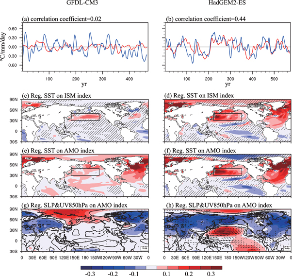
Figure 1. Temporal evolution of the AMO (red lines) and ISM (blue lines) indices in the control simulation for (a) GFDL-CM3 and (b) HadGEM2-ES (units: °C and mm/day). Regressions of the summer (June–September) SSTs onto the standardized ISM index for (c) GFDL-CM3 and (d) HadGEM2-ES. (e), (f) As in (c), (d) but for the AMO index. Black slashed lines indicate areas that are not statistically significant at the 95% confidence level, based on the t-test (units: °C/std). (g), (h) As in (e), (f) but for SLP (shading) and horizontal wind at 850 hPa (vector). Black lines indicate statistical significance at the 95% confidence level based on the t-test (units: hPa/std). For the wind, only regions where the wind is statistically significant at the 90% are shown. The reference wind speed is 0.3 m/s/std and given in the lower-right corner.
Download figure:
Standard image High-resolution imageCorresponding to the absence of AMO-ISM correlation in the control simulation of GFDL-CM3 (figure 1(a)), there are obvious differences between the ISM-related SST regression pattern and the AMO-related SST pattern for boreal summer; plus, their spatial correlation coefficient is low (r = 0.10) over the Atlantic and Pacific region (30°S–60°N, 130°E–360°E) (figures 1(c) and (e)). In comparison, for HadGEM2-ES, the AMO SST regression pattern resembles the ISM-related SST pattern, and their spatial correlation coefficient is high (r = 0.91) (figures 1(d) and (f)). Specifically, for the North Atlantic, GFDL-CM3 is characterized by a tripole-like SST pattern during the positive ISM phase (figure 1(c)) and has no correlation (r = 0.12) with the AMO pattern (figure 1(e)). HadGEM2-ES shows a basin-scale North Atlantic warming during the positive ISM and AMO phases (r = 0.91) (figures 1(d) and (f)). Despite these differences, one common feature is that the warmest SST anomalies occur in the central North Pacific (box in figure 1) during the positive ISM phase in both models (0.07 °C/std for GFDL-CM3; 0.14 °C/std for HadGEM2-ES). This indicates that the ISM is positively correlated with the SST anomalies in the North Pacific region (figures 1(c) and (d)). In other words, the North Pacific is a key region for the ISM. This is in agreement with previous studies (Feudale and Kucharski 2013, Joshi and Kucharski 2017, Luo et al 2017), which suggest that an extratropical-tropical SST gradient in the North Pacific corresponds to an enhanced Walker Circulation and more Indian summer rainfall. However, the two models perform differently in simulating the North Pacific signals linked to the AMO. In GFDL-CM3, the AMO-related SST regressions show weak anomalies in the North Pacific (−0.1 to 0.1 °C/std), whereas there are evidently stronger anomalies with a warm center in HadGEM2-ES (−0.15 to 0.35 °C/std) (figures 1(e) and (f)).
In terms of the atmospheric circulation, a positive AMO phase in GFDL-CM3 is associated with low-pressure anomalies over the North Atlantic and weak SLP anomalies over the North Pacific, as well as weak horizontal wind anomalies at 850 hPa (figure 1(g)); while HadGEM2-ES has significant high-pressure anomalies over the North Pacific and easterly anomalies along the equatorial Pacific, despite low-pressure anomalies over the North Atlantic (figure 1(h)). These differences in the AMO-related atmospheric circulation between the two models may lead to the differences in the SST anomalies and the extratropical-tropical gradient in the North Pacific (figures 1(e)–(f)). The differences in the teleconnection between the North Atlantic and the North Pacific might be a reason for the differences in simulating the AMO-ISM correlations. This is supported by the results of CMIP5 models, which suggest the Pacific pathway (i.e. a positive AMO leads to an extratropical-tropical gradient in the North Pacific and enhanced Walker Circulation) is one of the two crucial physical mechanisms for the AMO-ISM connection (Luo et al 2017).
Many previous studies have documented that a modification of the Walker Circulation induced by SST anomalies over the tropical Atlantic related to the AMO is responsible for the teleconnection between the North Atlantic and Pacific (McGregor et al 2014, Kayano and Capistrano 2014, Kucharski et al 2016). The physical mechanism is that, during the positive AMO phase, a warmer tropical Atlantic may lead to ascending motion and divergence in the Atlantic but descending motion and convergence in the central Pacific, at the upper level (Kucharski et al 2016). Comparing the AMO-related SST anomalies in the two models, it is clear that the warm anomalies in the tropical Atlantic are weaker in GFDL-CM3 (figure 1(e)) than in HadGEM2-ES (figure 1(f)) and the observation (figure S5(b)). The weak AMO-related SST anomalies in the tropical Atlantic in GFDL-CM3 are likely to be one of the reasons for the weak AMO-related atmospheric circulation. In addition, the weak AMO-related SST anomalies in the sub-tropical North Atlantic can also play a role in the existence of an incorrect teleconnection between the Atlantic and Pacific (Farneti 2017).
Comparing the variabilities of the AMO and the SST over the North Atlantic in the two models, GFDL-CM3 (standard deviation: 0.08 °C) is obviously weaker than HadGEM2-ES (standard deviation: 0.19 °C) and the observation (standard deviation: 0.15 °C) (figure S6). Furthermore, none of its first three EOFs show significant correlation with the AMO or the AMO-related SST pattern (table S1). The first leading EOF (24.2%) (figure 2(a)) shows much stronger positive SST anomalies over the tropical Pacific compared with the observation (figure S7), which might reduce the impact of the AMO on the North Pacific SST and the ISM. For HadGEM2-ES, the third leading EOF (6.2%) (figure 2(b)) shows high positive correlations with time series of the AMO and its SST regression pattern (table S1). This suggests that, in HadGEM2-ES, the simulated AMO is a major mode in the control simulation, while in GFDL-CM3 the simulated AMO variability is too weak to achieve its impact. Thus, we speculate that the AMO's amplitude may play a role in triggering a teleconnection with the Pacific. We will seek verification of this speculation in future work by using more CMIP5 models.

Figure 2. (a) The first leading EOF of summer (June–September) global filtered SSTs in the control simulation for GFDL-CM3. (b) As in (a) but for the third EOF in HadGEM2-ES. Values in the top right-hand corner indicate the percentage of variance explained. The EOFs are significantly separated.
Download figure:
Standard image High-resolution imageThese analyses show that the AMO in HadGEM2-ES exhibits a teleconnection with the North Pacific characterized by high-pressure and warm SST anomalies. Meanwhile, GFDL-CM3 fails to capture the signals over the North Pacific. This is the reason that the two models show different AMO-ISM correlations. This teleconnection of the AMO with the North Pacific has been documented in many previous studies (e.g. Dong et al 2006, Zhang and Delworth 2007, Kucharski et al 2016, Nagy et al 2016, Luo et al 2017, Ruprich-Roberts et al 2017, Sun et al 2017), and has been seen in observations (figures S5(b)–(c)). Hence, the simulations in HadGEM2-ES are more likely to be reasonable. We therefore suggest that the positive AMO-ISM correlation is likely to be intrinsic to the climate system. This study also indicates that the SSTs in the North Pacific should be considered when investigating the impacts of the AMO. This provides a benchmark for evaluating the skill of model in simulating the AMO's impact. Besides, it reveals the possibility that GFDL-CM3 may have certain defects in simulating the AMO-related Pacific signals, and thus provides hints for improving the model.
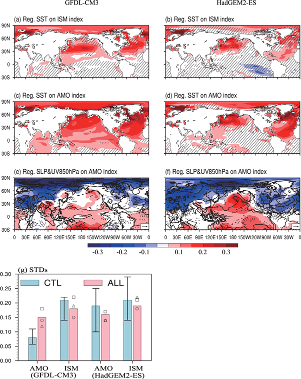
A remaining issue is why the two models show the same significant positive AMO-ISM correlation in their historical simulations. In terms of spatial characteristics, the SST regressions show that both the positive AMO and ISM are related to warm SST anomalies in the North Pacific and the North Atlantic in the two models (figures 3(a)–(d)), as seen in the observations (figure S5). However, the control simulation of GFDL-CM3 is unable to capture the AMO-related atmospheric circulations (see figures 1 and 3). This suggests that the external forcing in the historical simulation of GFDL-CM3 plays the key role in reproducing the North Pacific signals. By contrast, HadGEM2-ES shows no obvious difference between the control and historical simulations (figures 1 and 3).
Figure 3. Ensemble mean regressions of summer (June–September) SSTs onto the standardized ISM index for the historical simulation in (a) GFDL-CM3 and (b) HadGEM2-ES. (c), (d) As in (a), (b) but for the AMO index. Black slashed lines indicate areas that are not statistically significant at the 95% confidence level, based on the t-test. (units: °C/std). (e), (f) As in (c), (d) but for SLP (shading) and horizontal wind at 850 hPa (vectors). Black lines indicate statistical significance at the 95% confidence level based on the t-test (unit: hPa/std). For the wind, only regions where the wind is statistically significant at the 90% are shown. The reference wind speed is 0.15 m/s/std and given in the lower-right corner (unit: m/s/std). (g) Standard deviations of the AMO and ISM indices for the control (blue) and historical (red) simulations. Error bars stand for the range of the standard deviations calculated from a sliding window of 127 years over the control simulations. Circles, squares and triangles represent the values of runs 1, 2 and 3 of the two models, respectively. Units are °C for the AMO and mm/day for the ISM.
Download figure:
Standard image High-resolution image
The AMO indices in the historical simulations of the models show a significant positive correlation with the observations, implying that external forcing is important for the timing of the AMO phases in both models (table 1 and figure S2), which is in agreement with previous studies (Otterå et al 2010, Booth et al 2012, Chylek et al 2014). Although there is still much debate regarding the AMO response to external forcing (Zhang et al 2013, Chylek et al 2014), a detailed discussion of external forcing is beyond the scope of this study.
Table 1. Correlation between the modeled indices and observations. Correlations significant at the 95% level are shown in bold. 'Ens.' indicates the ensemble mean of the three members.
| Model | No. | AMO | ISM |
|---|---|---|---|
| GFDL-CM3 | r1 | 0.39 | −0.23 |
| r2 | 0.58 | −0.27 | |
| r3 | 0.60 | 0.48 | |
| Ens. | 0.60 | −0.01 | |
| HadGEM2−ES | r1 | 0.60 | −0.26 |
| r2 | 0.63 | 0.57 | |
| r3 | 0.58 | 0.55 | |
| Ens. | 0.69 | 0.40 |
One may note that, unlike the AMO, the correlation coefficients between the modeled ISM indices and the observations show a considerable range, from −0.27 to 0.55. This may be due to the ISM not only being largely dependent on the internal variability (table 1), but also being regulated by external forcing (e.g. Bollasina et al 2011, Guo et al 2015). The observed ISM is the combined results of internal variability and external forcing, not just the AMO. This is also seen from some traces of external forcing, like the wet phase in the middle 20th century and the dry phase in the 1970s (figure S2).
Comparing the standard deviations of the AMO indices in the historical simulation with those in the control simulation, the variability increases by roughly 0.06 °C in GFDL-CM3, and the variability varies within the ranges of the control simulation in HadGEM2-ES (figure 3(g)). Hence, external forcing has different effects on the AMO in the two models and these are mainly manifested in the tropical North Atlantic (figure S8). This difference may be a result of the large uncertainties in simulating clouds, given that aerosols can affect the tropical branch of the AMO due to feedbacks from clouds (Bellomo et al 2016, Brown et al 2016, Yuan et al 2016). For the ISM, the variabilities in the historical simulation fall into the variation ranges of the control simulation in both models (figure 3(g)). Hence, external forcing can synchronize the internal variability of the AMO, instead of generating new variability in HadGEM2-ES; whereas, it can synchronize and increase the variability of the AMO in GFDL-CM3. Subsequently, the significant increase in the variability in GFDL-CM3 may help to enhance air–sea interactions, and result in remote impacts on the North Pacific and the ISM.
4. Summary
This study uses two climate models (GFDL-CM3 and HadGEM2-ES) to address the issue of whether the positive correlation between the AMO and ISM since the Industrial Revolution is inherent to the climate system or caused by external forcing. Both models reproduce the observed AMO-ISM connection in all their historical simulations, but only one reproduces the connection in the control run with fixed preindustrial forcing. Our main results are as follows:
- (1)GFDL-CM3 shows no correlation (0.02) between the AMO and ISM in its control simulation, while HadGEM2-ES shows a significant positive correlation (0.44) in the same control run. Such a difference between the two models is due to their different simulations of the teleconnection of the AMO with the North Pacific, which is known to exist according to observations and previous studies (i.e. a positive AMO leads to warming SSTs over the North Pacific via air–sea interaction, which further induce easterly anomalies along the equatorial Pacific, and then enhance the ISM). HadGEM2-ES can simulate such a teleconnection reasonably, whereas GFDL-CM3 fails to simulate the AMO-related signals in the North Pacific. Hence, we suggest that the AMO-ISM connection is likely to be intrinsic to the climate system, and the North Pacific acts as an intermediary in the connection.
- (2)Comparisons of the control simulation with the historical simulation in GFDL-CM3 indicate that external forcing synchronizes and enhances the variability of the AMO, which could therefore have a larger effect on the global climate/teleconnections. External forcing mainly synchronizes the internal variability in HadGEM2-ES. The different responses to external forcing in the two models lead to the same AMO-ISM correlation in the historical simulation.
Acknowledgments
We thank the two anonymous reviewers for their valuable comments and suggestions, which helped greatly towards improving the manuscript. This study was jointly supported by the National Key R&D Program of China (Grant No. 2018YFA0606403), the National Natural Science Foundation of China (Grant Nos. 41790473, 41731177 and 41421004), and the Strategic Project of the Chinese Academy of Sciences (Grant No. XDA11010401).