

Abstract
Precise descriptions of forest productivity, biomass, and structure are essential for understanding ecosystem responses to climatic and anthropogenic changes. However, relations between these components are complex, in particular for tropical forests.
We developed an approach to simulate carbon dynamics in the Amazon rainforest including around 410 billion individual trees within 7.8 million km2. We integrated canopy height observations from space-borne LIDAR in order to quantify spatial variations in forest state and structure reflecting small-scale to large-scale natural and anthropogenic disturbances.
Under current conditions, we identified the Amazon rainforest as a carbon sink, gaining 0.56 GtC per year. This carbon sink is driven by an estimated mean gross primary productivity (GPP) of 25.1 tC ha−1 a−1, and a mean woody aboveground net primary productivity (wANPP) of 4.2 tC ha−1 a−1. We found that successional states play an important role for the relations between productivity and biomass. Forests in early to intermediate successional states are the most productive, and woody above-ground carbon use efficiencies are non-linear. Simulated values can be compared to observed carbon fluxes at various spatial resolutions (>40 m). Notably, we found that our GPP corresponds to the values derived from MODIS. For NPP, spatial differences can be observed due to the consideration of forest successional states in our approach.
We conclude that forest structure has a substantial impact on productivity and biomass. It is an essential factor that should be taken into account when estimating current carbon budgets or analyzing climate change scenarios for the Amazon rainforest.
Export citation and abstract BibTeX RIS

Original content from this work may be used under the terms of the Creative Commons Attribution 3.0 licence.
Any further distribution of this work must maintain attribution to the author(s) and the title of the work, journal citation and DOI.
Introduction
The terrestrial biosphere represents an important, but also an uncertain component of the global carbon cycle (Le Quéré et al 2016). In particular, the Amazon rainforest, which accounts for 50% of carbon stored in tropical forests (Pan et al 2011), takes a great share of this uncertainty. Estimates on stocks (Mitchard et al 2014) and fluxes (Johnson et al 2016, Castanho et al 2016) diverge for several reasons. On the one hand, the Amazon shows regional differences in mean wood densities and turnover rates although the drivers are still not entirely understood (Chave et al 2006, Malhi et al 2006, 2015). On the other hand, the Amazon is exposed to disturbances such as wind blow-downs (Chambers et al 2013, Fisher et al 2008), droughts (Phillips et al 2009, Gatti et al 2014), and deforestation (van der Werf et al 2009, Pütz et al 2014, Poorter et al 2014). Such disturbances shift forests into earlier successional states and influence forests' species composition and structure (Feldpausch et al 2011, Dubayah et al 2010), factors that are often neglected in large-scale estimates of the carbon budget (Houghton 2005).
In many global vegetation models, net primary productivity is mainly related to the amount of standing biomass (Johnson et al 2016). Thereby, models miss out on accounting for the effect of forest structure on productivity. Recent field studies deliver valuable analyses on potential drivers for the spatial variation of biomass and productivity within the Amazon rainforest. It was found that forest dynamics and hence biomass and productivity might be related to seasonality (Chave et al 2006, Malhi et al 2015, Hofhansl et al 2014) or soil properties (soil phosphorus and soil physical properties, Quesada et al 2017). It is, however, challenging to derive relations from field studies for large regions as the number and sizes of sample plots may not always be sufficient to be representative of an entire landscape (Marvin et al 2014). Analyses of the relation between biomass stocks and climatic conditions in the Amazon are based on ca. 300 one-hectare plots (e.g. Malhi et al 2006), and analyses of biomass increments on even less (ca. 200, Brienen et al 2015a, 2015b). More detailed analyses on carbon partitioning into gross and net primary production, for example, are based on an even smaller number of plots (e.g. 10 plots in Malhi et al 2015). An additional limitation lies in the fact that field studies do not account for the full range of successional states, forest structure, and species composition.
In this study, we present an approach that links a canopy height map with an Amazon-wide forest gap model (Rödig et al 2017a). Forest gap models simulate forest succession at the individual tree level. In our regionalization approach, precipitation and clay content of the soil are taken as a proxy for tree mortality which is supported by relations observed in the field (Quesada et al 2017). This relation was found to reproduce spatial differences in forest succession (Rödig et al 2017a). Spatially variable mortality rates are of particular importance in highly dynamic forests where small-scale mortality events can have a strong effect on forest carbon stocks (Espírito-Santo et al 2014). In addition, our forest model simulates forest structure and species compositions throughout all successional states. The linkage with the remotely sensed canopy height map derived from spaceborne LIDAR data (measurements in 2005, Simard et al 2011) allows for deriving the current state of the forest at a specific location, considering disturbance at different spatial scales under spatially heterogeneous environmental conditions.
Our approach allows for presenting static maps of carbon fluxes such as gross primary productivity (GPP), above-ground woody net primary productivity (wANPP), and net ecosystem productivity (NEP) for the Amazon rainforest. Simulation results were compared to previous mean global maps derived from MODIS (Zhao and Running 2010), up-scaled eddy flux measurements FLUXCOM (Jung et al 2017, Tramontana et al 2016), forest inventories (Malhi et al 2015, Brienen et al 2015a), and measurements at two eddy-flux towers (FLUXNET, GF-Guy, BR-Sa3). In addition, relations between above-ground biomass (AGB), carbon fluxes, and successional states are explored at various spatial resolutions (≥40 m).
In this study we address the following questions: (a) How do successional states of forests influence the carbon dynamics of the Amazon? (b) How do carbon fluxes vary spatially across the Amazon region? (c) Is the spatial variability of GPP and NPP in the Amazon rainforest mainly driven by standing biomass?
Methods
Study region
The study region covers 7.8 million km2 of forests in South America that are categorized as rainforest or moist deciduous rainforest (fewer than 5 dry months in which precipitation (mm) ≤2 times mean temperature (°C) (FAO 2001)), have an annual mean temperature above 18 °C, are located at an elevation below 1000 m and have an AGB >20 t ha−1 (Rödig et al 2017a).
An Amazon-wide individual-based forest gap model
Our analyses are based on a regionalized Amazon-wide version (Rödig et al 2017a) of the forest gap model FORMIND, which has already been applied at various locations in the tropics (Fischer et al 2016). The forest gap model is driven by mean photosynthetic photon flux density (PPFD), mean precipitation (both 0.5°, mean over 2003–2012, Weedon et al 2014), and clay fraction of soil (8 km, Wieder et al 2014). It simulates forest dynamics at the individual tree level considering the following main processes at a yearly time step: tree growth, competition, establishment, and mortality. Growth of an individual tree depends on its location within the forest community, where trees compete for light and space. A gain in tree biomass results from the difference between photosynthesis and respiration losses. A seedling can establish if light intensity on the forest floor is sufficient.
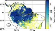
Figure 1. Map of simulated successional states of forests in the Amazon rainforest (for 2005). The simulated basal area fraction of late successional trees is used to classify the forest into different successional states: early successional state with basal area fractions of late successional trees <0.25, early-mid successional state with fractions between 0.25 and 0.50, mid-late successional state with fractions between 0.50 and 0.75, and late successional state with fractions >0.75.
Download figure:
Standard image High-resolution imageIn our model, tree mortality is an important driver for forest dynamics. Mortality increases when tree crowns are limited in space (crowding). Falling of large trees can damage surrounding trees (gap building) which causes conditional mortality events. In addition, every tree underlies a basic mortality rate which is determined stochastically. The characteristic of the Amazon-wide forest model is that this basic mortality rate varies spatially depending on temporal mean precipitation and the fraction of clay content in soil (Rödig et al 2017a). That means that in the model, mortality rates vary in space, but not in time. Hence, the forest model accounts for regional forest dynamics under mean climate conditions but does not consider inter-annual climate anomalies. Dead biomass is transferred to a dead wood carbon pool from which carbon is constantly transferred to a soil carbon pool (decomposition) or respired to the atmosphere.
The exchange of carbon between the forest and the atmosphere (net ecosystem productivity NEP [tC ha−1 a−1]), which is sometimes also referred to as net biome productivity (e.g. Jung et al 2011), is described as follows (Paulick et al 2017, Sato et al 2007):
The sum of gross primary productivity (GPPtree [tC ha−1 a−1]) minus autotrophic respiration (Rtree [tC ha−1 a−1]) over all tress equals the woody above-ground NPP (wANPP) of the forest site ([tC ha−1 a−1]). Autotrophic respiration Rtree is calculated as the sum of maintenance and growth respiration which also includes root respiration (figure S1 available at stacks.iop.org/ERL/13/054013/mmedia). Its annual rate is calculated in order to fit observed above-ground biomass growth of a tree. We assume that wANPP is a constant fraction of NPP (NPP = 2.72wANPP, derived for mature forests from Anderson-Teixeira et al 2016). Sdead is the dead wood pool, Sslow the slow decomposing soil carbon pool and Sfast the fast decomposing soil carbon pool (all [tC ha−1]) with its respiration rates to the atmosphere (tDA Sdead: to atmosphere, tSA: Sslow to atmosphere, tFA: Sfast to atmosphere, table S1).
The advantage of simulating each tree individually is that changes in forest structure are captured throughout all different successional states with different species compositions: from bare ground to climax stage including natural tree death. Differences in species composition are represented by three plant functional types: early successional, mid successional and late successional tree types that differ mainly in productivity, light needed at establishment, and mortality rates (table S1). Forest dynamics differ spatially as spatial variable mortality rates cause changes in competition between PFTs. This study focuses on the impact of forest structure on carbon fluxes under mean climatic conditions. This means that tree growth is limited to light and space, but trees grow (in the mean) under mean annual temperature and water conditions.
Technically, the individual-based model could simulate tree growth for every tree in the Amazon rainforest. However, the computational effort can be reduced for areas with similar environmental conditions at 1 km2 resolution. That means that for every area with similar environmental conditions (in total 1280 areas with similar mean precipitation, mean photosynthetic photon flux density (PPFD), and clay content, Rödig et al 2017a), only one model realization on 1 km2 (100 ha) is performed representatively (figure S2). Our simulation represents 7.8 million km2 of forest with 410 billion individual trees (>10 cm). Forest succession is simulated over 1000 years from bare ground to climax state (figure S3) on a high-performance Unix cluster.
Identifying the state of the Amazon rainforest
The successional state of each forest site within the Amazon is identified via a canopy height map (Simard et al 2011) as in Rödig et al (2017a). The canopy height map is based on space-borne LIDAR measurements taken aboard ICESat in May and June 2005. Consequently, the identified successional state of the forests represents the state in 2005. For each location in the Amazon rainforest (1 km2), we selected the simulated successional states to which the simulated canopy height equals the height given by the canopy height map. A successional state of the forest is here described as the basal area fraction of late successional trees (figure 1). We could then identify the forest's current carbon stock and its associated carbon fluxes (figure S2).
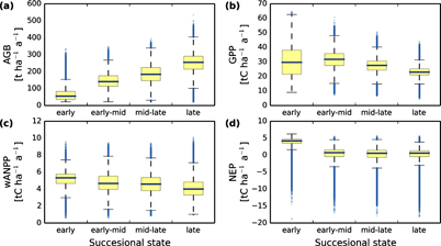
Figure 2. Estimated (a) above-ground biomass (AGB), (b) gross primary productivity (GPP), (c) woody aboveground net primary productivity (wANPP), (d) net ecosystem productivity (NEP) for forests in the Amazon, analyzed for different successional states (spatial resolution 0.16 ha, 4.8 billion simulated forest plots). The simulated basal area fraction of late successional trees is used to classify the forest into different successional states as in figure 1. The is shown as a blue horizontal line and outliers (outside whiskers) as blue dots.
Download figure:
Standard image High-resolution imageThe canopy height map comes with a root mean square error of 6.1 m at 1° resolution (Simard et al 2011). We performed an error analysis on how this uncertainty influences simulated GPP, wANPP, and NEP (see supporting information S1). This also includes those uncertainties that result from simulated canopy height and their different identified states. In addition, we tested how fluxes change when keeping the mortality rate constant throughout the Amazon (table S3).
Cross-comparison and validation
We compared our simulation results against observed NPP and GPP values from ten inventory sites in the lowland Amazon rainforest (Malhi et al 2015), measured woody above-ground net primary productivity (wANPP) from 193 sites (Brienen et al 2015a, 2015b), and GPP and NEP from two eddy covariance sites (<1 km2 footprint, annual means between 2004–2014, GF-Guy, Bonal et al 2008, annual means between 2000–2004, BR-Sa3, Goulden et al 2004). Please, note that the eddy covariance method observes the entire net ecosystem exchange (NEE) and we assumed here –NEE = NEP (Chapin et al 2006). Global mean GPP and NPP estimates from MODIS at 1 km2 resolution for the years 2000–2010 (Zhao and Running 2010, Running et al 2004) and GPP estimates from FLUXCOM at 0.5° resolution for the years 2000–2010 (mean over all realizations of different machine learning methods, Jung et al 2017, Tramontana et al 2016) were remapped (nearest neighbor, CDO 2015) to the resolution of our map to be compared against our simulation results.
Table 1. Mean ± standard deviation across Amazon rainforest (at 1 km2 resolution) of gross primary productivity (GPP), net primary productivity (NPP), net ecosystem productivity (NEP), and above-ground biomass (AGB) over 7.8 million km2 for four sub-regions (according to Feldpausch et al 2011, figure S11) derived from three different approaches: FORMIND, MODIS and FLUXCOM.
| FORMIND | MODIS | FLUXCOM | |||||
|---|---|---|---|---|---|---|---|
| Mean GPP ± std tC ha−1 a−1 | Mean NPP ± std tC ha−1 a−1 | Mean NEP ± std tC ha−1 a−1 | Mean AGB ± std t ha−1 | Mean GPP ± std tC ha−1 a−1 | Mean NPP ± std tC ha−1 a−1 | Mean GPP ± std tC ha−1 a−1 | |
| Western Amazon | 24.7 ± 3.0 | 10.2 ± 2.9 | 0.7 ± 1.2 | 208 ± 120 | 27.9 ± 4.8 | 13.2 ± 4.6 | 29.1 ± 6.1 |
| Brazilian Shield | 25.6 ± 3.9 | 12.4 ± 2.7 | 1.2 ± 1.7 | 123 ± 112 | 23.4 ± 3.9 | 8.5 ± 2.3 | 25.9 ± 4.8 |
| East Central Amazon | 24.7 ± 2.8 | 11.7 ± 2.3 | 0.5 ± 1.1 | 218 ± 86 | 25.2 ± 2.6 | 8.8 ± 2.6 | 30.3 ± 2.1 |
| Guiana Shield | 25.0 ± 2.2 | 10.7 ± 2.7 | 0.3 ± 0.8 | 255 ± 93 | 24.8 ± 2.3 | 9.9 ± 1.8 | 31.1 ± 3.1 |
| Amazon region | 25.1 ± 3.2 | 11.3 ± 2.8 | 0.7 ± 1.4 | 188 ± 120 | 25.4 ± 4.2 | 10.3 ± 3.7 | 28.8 ± 5.1 |

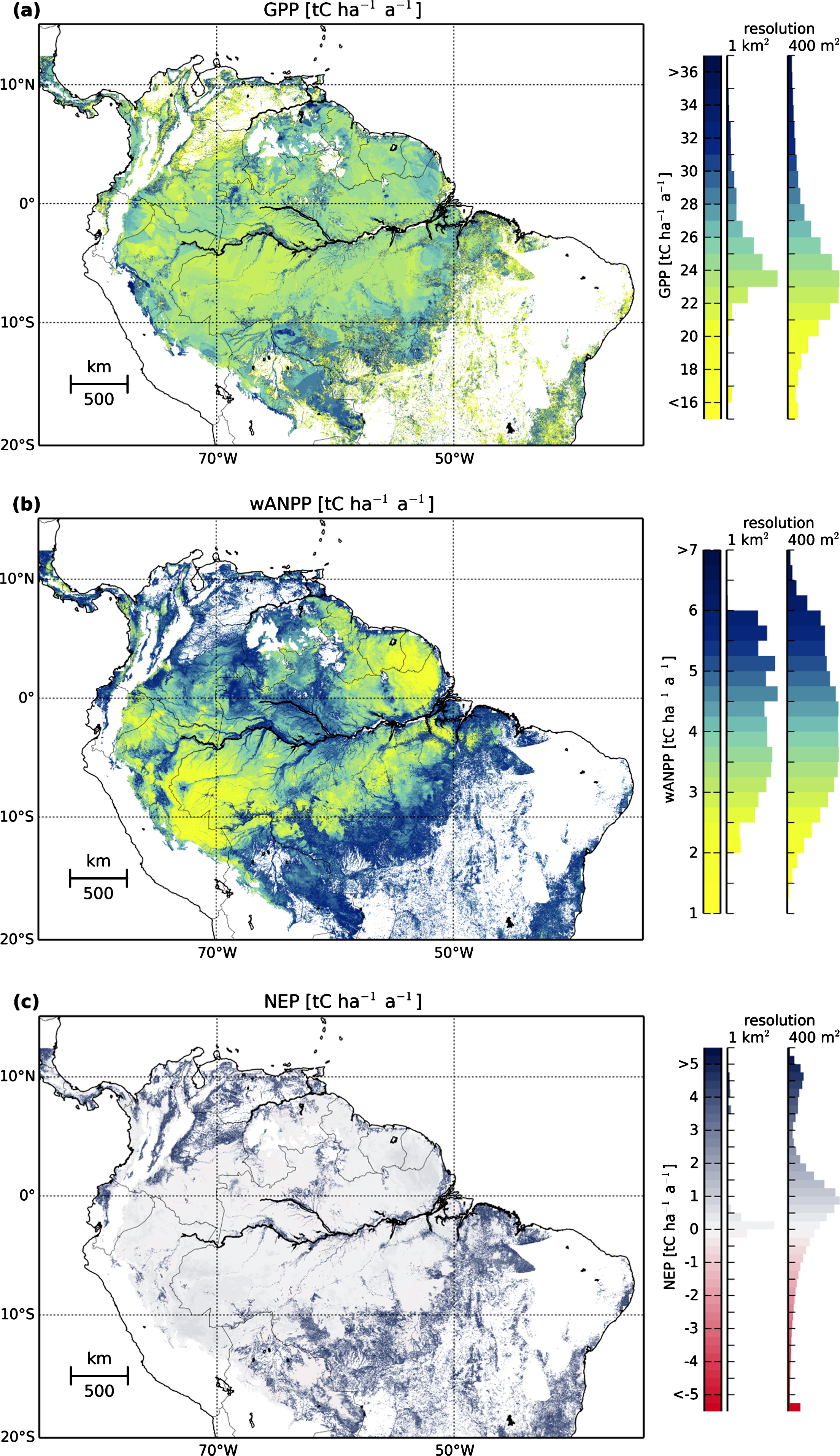
Figure 3. Maps and frequency distributions (normalized) under mean climate conditions of (a) gross primary productivity (GPP), (b) woody above-ground net primary productivity (wANPP), and (c) net ecosystem productivity (positive values indicate a sink of atmospheric carbon), estimated by linking simulations of the forest model FORMIND with a canopy height map. Note that our NEP estimates does not include the carbon emitted due to fire and deforestation (see methods). The maps represent the time when LIDAR measurements were taken (2005). The maps and the left histograms have a resolution of 1 km2. The right histograms have a resolution of 0.16 ha. Note that the mean values for both frequencies are the same.
Download figure:
Standard image High-resolution image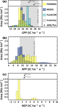
Figure 4. Frequency distributions of FORMIND estimates for (a) gross primary productivity (GPP), (b) net primary productivity (NPP), and (c) net ecosystem productivity (NEP) for forests in the Amazon at 1 km2 resolution in comparison to: estimates from MODIS (1 km2 resolution), FLUXCOM (0.5° resolution), inventory data (≤1 ha resolution, 10 plots with recorded GPP and NPP, Malhi et al 2015), and eddy covariance measurements (GF-Guy and BR-Sa3). The ranges of estimated values from field inventories are marked in grey. Mean eddy-flux values are plotted as grey dots. Note that positive values of NEP define a sink of atmospheric carbon.
Download figure:
Standard image High-resolution image
Figure 5. Differences of (a) gross primary productivity (GPP) and (b) net primary productivity (NPP). MODIS derived values (mean values 2000–2010) and the approach presented here (FORMIND).
Download figure:
Standard image High-resolution image
Figure 6. Relation between simulated carbon fluxes and successional states within the Amazon rainforest at a resolution of 0.16 ha (4.975 billion plots; Figure S4 for 1 ha resolution). Successional states are represented by the simulated basal area fraction of late successional trees within each 0.16 ha plot (as in figure 1). (a) Woody above-ground net primary productivity (wANPP) vs. above-ground biomass (AGB), (b) gross primary productivity (GPP) vs. AGB, (c) wANPP vs. GPP, and (d) net ecosystem productivity (NEP) vs. AGB. GPP, NEP and wANPP are in tons carbon per hectare per year (tC ha−1 a−1); AGB values are in tons dry mass per hectare (t ha−1).
Download figure:
Standard image High-resolution image
Results
Dynamics of forests in different successional states
By linking vegetation modelling with canopy height map information from remote sensing (Simard et al 2011), we were able to derive the successional state of forests in the Amazon rainforest (figure 1), here as basal area fraction of late successional trees. AGB increases throughout the successional state of a forest as expected (figure 2, figure S5 for additional attributes) while GPP peaks at early-mid successional state and is significantly higher than in mid-late and late successional state. wANPP decreases with successional state of the forest. NEP is significantly higher in early successional than in late successional state. NEP is around 0 in mid-late to late successional state. All fluxes in all states show significant differences (except NEP in mid-late and late successional state).
Spatial distribution of GPP, wANPP and NEP at different spatial scales
Across the Amazon basin, we obtain a mean GPP of forests of 25.1 tC ha−1 a−1 (figure 3(a), table 1). GPP values are higher along the Amazon river and in the southern Amazon rainforest (figure 3(a)). The pattern of woody aboveground productivity (wANPP, figure 3(b)) resembles the one of GPP with higher values along the rivers and in the southern Amazon. Mean wANPP is 4.2 tC ha−1 a−1. In some parts of the Amazon (e.g. the Guiana Shield), GPP values are higher than the mean while wANPP values are lower than the mean. NEP varies around zero (figure 3(c)) with a mean NEP value of 0.7 tC ha−1 a−1. NEP values of up to 5 tC ha−1 a−1 are reached only along the south-east and north-west.
The variation of GPP, wANPP, and NEP values at small scales (0.16 ha resolution) is higher than the variation at 1 km2 resolution (frequency distributions in figure 3). For example, the analysis of NEP at 0.16 ha resolution shows that forests can release up to 20 tC ha−1 a−1 to the atmosphere (figure 2(d)), while its maximum release at 1 km2 is 0.23 tC ha−1 a−1. Within an area of 7.8 Mio km2, the Amazon rainforest takes up 0.56 GtC per year (emissions due to fire and outtake of wood are not included).
Comparison of simulation results with other flux estimates
We compare our obtained values at 1 km2 resolution (figure 4) with estimates derived from MODIS (1 km2 resolution, Running et al 2004, Zhao and Running 2010), FLUXCOM (0.5° resolution, Jung et al 2017, Tramontana et al 2016), inventory data (ca. 1 ha plots, Brienen et al 2015a, 2015b, Malhi et al 2015), and eddy-covariance measurements (<1 km2 footprint, FLUXNET stations GF-Guy and BR-Sa3).
Gross primary production: The overall frequency distribution of simulated GPP resembles the one derived from MODIS with a mean of 25 tC ha−1 a−1 (figure 4(a)). We observe slightly higher GPP values with MODIS than with our approach for forests in late succession while it seems to be inverse for forests in early succession (figure 5). FLUXCOM GPP is higher with a mean of 28.8 tC ha−1 a−1. GPP derived from inventory data (24–42 tC ha−1 a−1, Malhi et al 2015) and from eddy flux measurements at GF-Guy (32–40 tC ha−1 a−1, Bonal et al 2008) and BR-Sa3 eddy flux station (29–42 tC ha−1 a−1, Goulden et al 2004) fall into the upper ranges of our simulated GPP. A one-to-one comparison shows that eddy flux measurements are in rather good agreement with simulation results at the nearest location (figure S8).
Net primary production: MODIS NPP shows a similar pattern as the related GPP distribution and has a clearly defined peak at 9–10 tC ha−1 a−1 with a mean of 10 tC ha−1 a−1 (figure 4(b)). NPP simulated with FORMIND, on the other hand, is broadly distributed between of 8–16 tC ha−1 a−1. In contrast, if the entire region was assumed to be in climax state, there is a single well defined peak in the NPP distribution (figure S9). NPP values derived from forest inventory range from 9–16 tC ha−1 a−1 (Malhi et al 2015). Estimated wANPP from field inventories (Brienen et al 2015b) range from 1.1–4.7 tC ha−1 a−1, while FORMIND reaches high wANPP values of up to 6 tC ha−1 a−1 (figure S10). Note that the field inventories are limited to measurements (193 sites) mainly taken in old-grown forests.
Net ecosystem productivity: Simulated NEP values under mean climate conditions fall into the range of recordings at the GF-Guy eddy flux station (1.57 tC ha−1 a−1) and the BR-Sa3 station (1.65 tC ha−1 a−1).
Relation between analyzed carbon stocks, dynamics and species compositions
Figure 6 shows the obtained relations between carbon fluxes and stocks according to the successional state of a forest plot. Forests in early successional state reach AGB values of 100–150 t ha−1. Forests in early-mid and mid-late successional state reach values up to 300 t ha−1. Forests in late successional state have AGB values greater than 250 t ha−1.
wANPP and AGB stock show a bell-shaped relation (figure 6(a)). GPP values and AGB values form a triangle (figure 6(b)). Forests in early successional states reach higher GPP values than forests in late successional state (with the same AGB). Comparing both figures (a and b) in late successional states, it is evident that wANPP decreases with increasing AGB while GPP increases with AGB.
The relation between GPP and wANPP displays the woody above-ground carbon use efficiency which varies for different successional states (figure 6(c)). Low GPP values are reached for all successional states with a broad range of wANPP values. NEP is always positive for early successional forests, but NEP values of late successional forests show a large variation (figure 6(d)).
Error analysis
GPP values in our map come, on average, with a standard error of 4.15 tC ha−1 a−1 caused by the uncertainties in the canopy height map (figure S6(b), table S2). Errors in the GPP map are slightly higher for the Brazilian Shield (including the 'Arc of Deforestation') than for the other regions. wANPP has a mean standard error of 0.90 tC ha−1 a−1. Errors in wANPP are highest in East Central Amazon and West Amazon. NEP has an average standard error of 0.65 tC ha−1 a−1 and is highest for the Brazilian Shield where the error is 23% higher than the overall mean. All fluxes show lower uncertainties for the Guiana Shield.
When keeping mortality rates constant throughout the Amazon, the standard deviations across the Amazon stay more or less constant (table S3).
Discussion
In this study, we link individual-based simulations with remote sensing measurements to assess the Amazon rainforest's carbon stocks and fluxes.
Carbon fluxes and stocks at different successional states
Our analysis shows how the successional states of a forest (figure 1) influence carbon stocks and fluxes. Noticeably, wANPP, GPP, and NEP are highest for forests in early to mid-successional states (figures 2(c) and (d)). Such forests of high productivity can be found (figure 3), for example, along the 'Arc of deforestation' in the south-east (Nogueira et al 2008) where forests are degraded by human activities.
The successional state of a forest is not only influenced by large-scale disturbances, but also by individual tree mortality. This means that even undisturbed, large forests in mature state consist of different successional states at the small scale (e.g. 400 m2, figure S2) and can hence show fluctuations in its carbon dynamics. Chambers et al (2013) found, for example, that biomass of a mature forest is stable over time only for sample plots greater than 10 ha. For that reason, derived flux values at small scales show larger variability than at coarser resolution (frequency distributions at 400 m2 = 0.16 ha vs. 1 km2 resolution in figure 3, and figure 6 vs. Figure S4). This may be related to the finding of Espírito-Santo et al (2014) that individual tree mortality over the entire Amazon cause greater biomass losses than large-scale disturbances. Note here that our study includes the consequences of disturbances (regrowth from earlier successional state), but does not account for emissions due to fire or outtake of wood (logging).The relations derived here between simulated stocks and fluxes (figure 6) show that the amount of standing biomass (AGB) is not the only driver for productivity. Our derived relation between wANPP and AGB (figure 6(a)) is in agreement with a global field study which reports that highly productive forests may limit AGB values due to a dominance of species with low wood density (Keeling and Phillips 2007). Our relation therefore differs from simulation results of 4 DGVMs for the Amazon region presented in Johnson et al (2016). In their study, three DGVMs simulate increasing NPP with increasing AGB. Only one DGVM shows a slight reduction of NPP at high AGB values. They conclude that stem mortality rates need to be included in order to capture the relation between woody productivity and biomass as observed in the field (Johnson et al 2016). In our approach, we explicitly simulate stem mortality which is driven by a spatial variation of precipitation and clay content. As a consequence, spatial differences in dynamics and mean wood density are considered (Rödig et al 2017a). This is particularly important for the Amazon where carbon stocks and dynamics are driven by a spatial variation of mortality (Malhi et al 2015, Galbraith et al 2013, Quesada et al 2017, Baker et al 2004, Phillips et al 2004).
Limitations of our approach
The approach brings along structural uncertainties such as the simplified assumption that NPP is a constant fraction of wANPP, parameter uncertainties, and limitations due to the resolution of input data, here climatological data and the canopy height map (Simard et al 2011). The canopy height map is based on discrete LIDAR shots and provides estimates for canopy height at a resolution of 1 km2. Missing information between shots is a source for uncertainties in the map (Simard et al 2011). The effect these uncertainties on carbon fluxes is discussed below.
We here make simplifications regarding the handling of disturbance histories of the forests (i.e. fire event, logging). Currently, we cannot reconstruct the type of disturbance event from the canopy height map. Consequently, a disturbed forest site is based on the assumption that it either regenerates after deforestation (simulation from bare ground with initialized dead wood and soil pools, table S1), or is influenced by natural tree fall and its resulting mortality (gap-dynamics).
The study presented here focuses on the spatial variability in carbon dynamics resulting from forest structural and environmental differences under current climatic conditions. Consequently, results capture all fluxes for only one point in time (i.e. an average over the period 2003–2012 with structural information of the canopy height map in 2005, Rödig et al 2017a). The study design does not yet consider the effects of inter- or intra-annual variations of temperature or atmospheric CO2 on forest structure (Sakschewski et al 2015, Haverd et al 2013). It is anticipated to integrate such effects (as it has already been tested for temperate forests in Bohn and Huth 2017 and Rödig et al., 2017) into future work in order to also have the possibility effects of droughts.
Comparison with field data and remote sensing measurements
Testing the representativeness of our GPP map relies on the comparison with other maps derived from remote sensing and simulation (MODIS, Running et al 2004, Zhao and Running 2010) and upscaled eddy flux measurements (FLUXCOM, Jung et al 2017, Tramontana et al 2016). Direct carbon flux measurements in the Amazon rainforest are rare (10 inventory plots (Malhi et al 2015) and two eddy flux measurements) and only partly suitable for large-scale estimates.
GPP: The frequency distribution of the MODIS GPP (Running et al 2004, Zhao and Running 2010) resembles our simulated GPP distribution (figure 4(a)) although both maps are derived from different remote sensing techniques (NDVI vs. LIDAR) which lends confidence to our simulations. MODIS and FLUXCOM show particularly low GPP values for the Brazilian Shield for which FORMIND produces higher GPP values than for the rest of the Amazon (table 1, figure 5). These differences probably arise from the fact that our approach uses a representation of forest succession which leads to higher GPP values in early-mid successional states (figure 2(b)). This may also be the reason for differences in GPP values towards the Andes (figure 5, figure S7). In addition, discrepancies may arise from the fact that our approach includes spatial variable mortality rates which lead to differences in forest gap-dynamics across the Amazon. Our simulations at 1 ha resolution reach GPP values comparable to field observations (figure S4), whereas simulated values at 1 km2 are lower.
NPP: Our approach (figure 4(b)) displays more forests with high NPP values (>12 tC ha−1 a−1) than the MODIS product. Please note that the NPP pattern of the MODIS product correlates with its GPP pattern (table 1) whereas our approach indicates forest structure as an important additional factor (GPP vs. NPP, carbon use efficiency is not constant, figure 6(c), figure S5(a)). We identify two potential explanations for such discrepancy. First, the representation of different PFTs, which allows for simulating forest succession, leads to higher NPP values (figure 2(c)), especially in highly disturbed regions like the Brazilian shield (table 1). The successional state identified with the canopy height map seems to have more influence on NPP than internal gap-dynamics due to variable mortality rates (table S3). Second, the MODIS product, which is often used for global estimates (Jung et al 2017, Bloom et al 2016, Zhao and Running 2010), is limited by the fact that it is derived from Normalized Difference Vegetation Index (NDVI) values. The NDVI tends to saturate in dense mature forests and, thus, has limited capability to identify spatial variations, such as in the Amazon (Hall et al 2011, Myneni et al 2001). The method presented here uses a canopy height map (Simard et al 2011) that is derived from LIDAR measurements. Active remote sensing tracers (here LIDAR) have the advantage that they are highly sensitive to structural variations (Lefsky et al 2002).
NEP: We here estimate that the Amazon forest gains, on average, 0.56 Gt of carbon per year and as such yields a positive NEP. Even when considering a mean standard error of ±0.51 Gt of carbon per year due to uncertainties in the canopy height map, the Amazon is identified as a sink of atmospheric carbon. As this value is the potential carbon uptake due to the successional states of the forests, our estimate compensates approximately the amount of carbon currently released due to deforestation and land-use change in South America (Baccini et al 2012). In particular, forests in earlier successional states contribute to an uptake of atmospheric carbon (Poorter et al 2014, figure 2(d)).
Conclusion
In our study, we have shown that the successional state of forests, and hence forest structure and species composition, have a strong effect on NPP and NEP. This effect is reflected in higher NEP and wANPP values for forests that regrow after deforestation (Poorter et al 2014), particularly, along the Arc of deforestation and higher wANPP values in East-central Amazon due to internal gap-dynamics. Our results reveal that NEP across the Amazon is a carbon sink of 0.56 ± 0.51 Gt C per year driven by high productivity in regenerating forest areas, approximately offsetting estimates of fire and deforestation emissions. We show that AGB alone does not account for productivity differences (figure 6) and found that structure and species compositions are important as well.
Individual-based modelling at the large scale, such as the Amazon rainforest, is expensive in computational demand. However, a high-resolution approach allows for integrating observational data at different spatial scales and contributes to a better understanding of forest dynamics at the large scale. The approach can be expanded in future work by integrating further remote sensing data into the analysis. For example, matching vertical canopy profiles from LIDAR with simulated profiles (Knapp et al 2018) can provide additional insights into the actual successional state of forests. Our analyses highlight the importance of accounting for forest structure when simulating carbon dynamics. We therefore suggest that forest structure should also be incorporated in global dynamic vegetation modelling.
Acknowledgments
ER, RF, AR, and AH were supported by the Helmholtz-Alliance Remote Sensing and Earth System Dynamics. MC was supported by a grant overseen by the French National Research Agency (ANR) as part of the 'Investissements d'Avenir' program (ANR-11 L ABX-0002-01, Lab of Excellence ARBRE). We thank Martin Jung for providing FLUXCOM data, and Damien Bonal and FLUXNET for providing eddy covariance data. This work used eddy covariance data acquired and shared by the FLUXNET community, including these networks: AmeriFlux, AfriFlux, AsiaFlux, CarboAfrica, CarboEuropeIP, CarboItaly, CarboMont, ChinaFlux, Fluxnet-Canada, GreenGrass, ICOS, KoFlux, LBA, NECC, OzFlux-TERN, TCOS-Siberia, and USCCC. The ERA-Interim reanalysis data are provided by ECMWF and processed by LSCE. The FLUXNET eddy covariance data processing and harmonization was carried out by the European Fluxes Database Cluster, AmeriFlux Management Project, and Fluxdata project of FLUXNET, with the support of CDIAC and ICOS Ecosystem Thematic Center, and the OzFlux, ChinaFlux and AsiaFlux offices. We also thank Michael Müller, Sebastian Paulick and Matthias Zink for technical support. We greatly appreciate the constructive and thoughtful comments of the anonymous reviewers.