

Abstract
To assess the impact of anthropogenic aerosol emission reduction on limiting global temperature increase to 1.5 °C or 2 °C above pre-industrial levels, two climate modeling approaches have been used (MAGICC6, and a combination of ECHAM-HAMMOZ and the UVic ESCM), with two aerosol control pathways under two greenhouse gas (GHG) reduction scenarios. We found that aerosol emission reductions associated with CO2 co-emissions had a significant warming effect during the first half of the century and that the near-term warming is dependent on the pace of aerosol emission reduction. The modeling results show that these aerosol emission reductions account for about 0.5 °C warming relative to 2015, on top of the 1 °C above pre-industrial levels that were already reached in 2015. We found also that the decreases in aerosol emissions lead to different decreases in the magnitude of the aerosol radiative forcing in the two models. By 2100, the aerosol forcing is projected by ECHAM–UVic to diminish in magnitude by 0.96 W m−2 and by MAGICC6 by 0.76 W m−2 relative to 2000. Despite this discrepancy, the climate responses in terms of temperature are similar. Aggressive aerosol control due to air quality legislation affects the peak temperature, which is 0.2 °C–0.3 °C above the 1.5 °C limit even within the most ambitious CO2/GHG reduction scenario. At the end of the century, the temperature differences between aerosol reduction scenarios in the context of ambitious CO2 mitigation are negligible.
Export citation and abstract BibTeX RIS

Original content from this work may be used under the terms of the Creative Commons Attribution 3.0 licence.
Any further distribution of this work must maintain attribution to the author(s) and the title of the work, journal citation and DOI.
1. Introduction
The impact of anthropogenic aerosols on the Earth's radiative balance remains the single largest uncertainty in our understanding of current drivers of climate change [1]. Depending on their type, aerosols have the ability to perturb the radiative balance of the atmosphere, either directly by scattering and absorbing solar radiation, or indirectly via the modification of cloud properties. Any changes in aerosol concentrations therefore have the potential to intensify or attenuate the effects of anthropogenic climate change [2, 3, 4, 5, 6]. The net effect of all present-day atmospheric aerosols is estimated to be cooling, thus potentially counteracting a considerable fraction of the global warming associated with greenhouse gases (GHGs) [7].
The Paris agreement [8], reached in December 2015 under the auspices of the United Nations Framework Convention on Climate Change, aims to restrict global temperature increase to well below 2 °C above pre-industrial levels, and 'to pursue efforts to limit the temperature increase to 1.5 °C'. Reaching either of these goals will require net emissions of all long-lived greenhouse gases (LLGHGs) to be brought to zero as early as within the next few decades, and certainly before the end of this century [9, 10, 11]. This means that the total amount of anthropogenic LLGHGs that can ever be emitted into the atmosphere is finite [12]. For carbon dioxide (CO2), which is the dominant driver of long-term temperature increases [13], this finite amount is often referred to as a carbon budget. In 2016, Rogelj et al [17] estimated that in order to ensure a larger than 66% chance of limiting the global temperature increase to 2 °C, the remaining carbon budget from 2015 onwards is in the range of 590–1240 GtCO2, which is equivalent to between 15 and 30 years of present-day CO2 emissions.
However, new research suggests that the remaining budgets for very ambitious climate targets may be considerably larger than previously thought. In 2017, Millar et al [14] showed that the remaining CO2 budget for staying below the 1.5 °C limit is about four times greater than was estimated in the 2014 IPCC report [15]. Their conclusion emerged from the observation that the subset of earth system models used to estimate the lower limit of the carbon budget (i.e. the most sensitive 33% of models with respect to their response to CO2 emissions) simulated an almost 0.3 °C higher temperature change than has been observed in response to total historical CO2 emissions. After correcting for this bias, they estimated that the 66% carbon budget for 1.5 °C may be as large as 240 GtC (880 GtCO2). This new analysis introduces considerable new uncertainty into estimates of remaining carbon budgets, though it is also generally consistent with another recent independent estimate of the remaining budget for 1.5 °C [16].
Importantly, however, any estimate of allowable CO2 emissions is sensitive to the assumed scenario of non-CO2 forcers, including the non-CO2 GHGs (methane (CH4), nitrous oxide (N2O), halocarbons, etc) and the anthropogenic aerosols such as black carbon (BC), organic carbon (OC) and sulfate (SO4). Millar et al [14] assumed that non-CO2 forcings would follow RCP2.6 (Representative Concentration Pathway with a radiative forcing value of +2.6 W m−2 in the year 2100 relative to pre-industrial values), and their carbon budget results are therefore contingent on an arbitrary single scenario of non-CO2 emissions. Uncertainty associated with both the choice of emissions scenario and the magnitude of non-CO2 forcing is a large contributor to carbon budget uncertainty [17] given that increased (decreased) non-CO2 contributions to future warming will decrease (increase) the allowable CO2 emissions [16]. Given the large uncertainty associated with aerosol forcing in particular, it is important to better quantify the effect of aerosol uncertainty in the context of meeting ambitious climate targets.
In 2015, Rogelj et al [18] studied the effects of short-lived climate forcers on the 2 °C CO2 budget, and concluded that different aerosol (BC and SO4) emission scenarios have only a minor effect on the CO2 budget because staying below the 2 °C limit requires achieving zero CO2 emissions by the end of the century, and most of the aerosol emissions originate from combustion. In effect then, aerosol emissions would be expected to decrease greatly by 2100 in any emission scenario that succeeds in remaining below 2 °C. However, Rogelj et al [18] did not study how the different aerosol emission scenarios would affect temperature evolution in the decades before the end of the century, during the time when CO2 is still being emitted.
In addition, a number of scientific papers have touched on the question of how aerosol pollution control could affect the future global climate [19, 20]. For instance, in 2012 Mickley et al [21] conducted a series of climate simulations following a scenario of increasing GHG concentrations, with and without aerosols over the United States of America, and with present-day aerosols elsewhere. They found that the removal of all anthropogenic aerosol sources over the United States of America would lead to a significant regional warming over the period 2010–2050, with annual mean surface temperatures increasing by 0.4 °C–0.6 °C in the Eastern United States when compared with the reference year, 2010. Pietikäinen et al [22] simulated several aerosol control scenarios using a global climate model, and showed that targeted BC emission reductions are the most beneficial in terms of controlling climate warming. They found that the targeted BC reductions can lead to almost 0.8 W m−2 smaller (positive) radiative forcing by 2030 than maximum technologically feasible aerosol emission reductions do. Furthermore, in 2013, Sillmann et al [5] investigated the changes in extreme temperature and precipitation events over Europe under future scenarios of anthropogenic aerosol emissions. They showed that a global reduction in aerosol emissions can magnify the changes in temperature and precipitation extremes.
All these preceding articles highlight the role of aerosols and the importance of aerosol mitigation policies on the rate and magnitude of near-term climate change. Hence, the purpose of our study is to assess the impact of anthropogenic aerosol emission reductions on efforts to limit the temperature increase to 1.5 °C or 2 °C above pre-industrial temperatures. To do this, we will investigate several aerosol control pathways under two GHG reduction scenarios.
2. Methodology
This study utilizes two climate modeling approaches: firstly, a reduced-complexity model MAGICC (the Model for the Assessment of Greenhouse-gas Induced Climate Change) [23, 24] and, secondly, a combination of the detailed aerosol-climate model ECHAM-HAMMOZ [25, 26, 27] and the intermediate-complexity University of Victoria Earth System Climate Model (UVic ESCM) [28, 29]. Both models have different approaches, and generate complementary information. MAGICC—one of the primary models used in IPCC reports since 1990 to produce projections of future global mean temperatures—is more general and gives a probability range for the temperature increase. However, MAGICC does not have the capability of producing temperature and aerosol radiative forcing spatial distribution, providing only a general, 'broad-brush' view of the climate. Hence, the combination ECHAM–UVic has been introduced. Moreover, in order to manage the uncertainties that climate modeling is prone to, and to gain more confidence in the projections of climate change, the use of different types of global models is recommended. At this point we would like to underline the fact that the results of this study are based on simulations of only two climate models. As the two models do not span the full range of uncertainty of aerosol forcing, we do not regard these results as irrefutable, but we consider that aerosols and their effect on climate deserve more attention when discussing future aerosol emission regulations.
Two different GHG emissions for future scenarios were simulated: the RCP2.6 (otherwise known as RCP3PD) and a CO2 reduction scenario leading to a 1.5 °C increase in global mean temperature (see details in section 2.3). Each GHG emission scenario included two alternative aerosol emission control cases: the Current Legislation (CLE) scenario assumes currently-decided emission limits are enforced, and the Maximum Feasible Reduction (MFR) scenario assumes implementation of the current, most advanced technologies to drastically reduce aerosol emissions [30, 31]. These aerosol emission control strategies are described in detail elsewhere [32, 33].
2.1. MAGICC6
MAGICC is a reduced-complexity, probabilistic climate model that synthesizes current scientific understanding about many different gas cycles (including the carbon cycle), climate feedbacks and radiative forcing. MAGICC has a hemispherically averaged upwelling-diffusion ocean coupled to an atmosphere layer and a globally averaged carbon cycle model. The abundance of aerosols is approximated by changes in their hemispheric emissions, either from emissions scenarios or, if scenario data are not available, with proxy emissions (for instance, using CO as a proxy emission for OC and BC). This approach is justified due to the short lifetime of aerosols in the atmosphere. The direct effect of aerosols is approximated by simple linear forcing-abundance relationships for SO4, nitrate, BC and OC. The model version used in this study, MAGICC6, has been successfully calibrated against the higher complexity AOGCMs Atmosphere-Ocean Global Circulation Model and carbon cycle models. For a detailed description of MAGICC6, we direct the reader to the model description paper by Meinshausen et al [23]. For this study we used the online version of the model (live.magicc.org) run in both standard and 'probabilistic/historical constrained' setups that provide distributions of key climate outputs yearly and decadally, respectively. MAGICC6 in the probabilistic setup runs 600 simulations per scenario, matching the assessment of carbon cycle and climate uncertainties in the IPCC AR4 [34]. The temperature simulations are also constrained by observations of hemispherical temperatures and heat uptake.
2.2. ECHAM-HAMMOZ and UVic ESCM
As a second approach, we used a combination of two models. Firstly, the spatial and temporal variation of aerosol radiative forcing was simulated with a development version of the global aerosol-climate model ECHAM-HAMMOZ (version ECHAM6.1 HAM2.2–SALSA) [25, 26, 27]. ECHAM-HAMMOZ with prescribed sea surface temperature is unable to simulate climate responses such as a change in temperature due to the different emission scenarios. Therefore, secondly, the radiative forcing from ECHAM-HAMMOZ was interpolated spatially and temporally (see below for details) and fed into the UVic ESCM that was then used to calculate the climate response.
ECHAM-HAMMOZ consists of an atmospheric core model ECHAM, which solves the fundamental equations for the atmospheric flow and physics and tracer transport, and of an aerosol model HAM. SALSA describes the aerosol population consisting of SO4, sea salt, OC, BC, and dust, and uses ten size sections to cover the size range from 3 nm to 10 μm. HAM–SALSA considers: emissions of aerosols and of SO4 aerosol precursors; the temporal evolution of aerosols through aerosol microphysics module SALSA (i.e. nucleation, coagulation, growth through condensation of sulfuric acid, and hygroscopic growth) [27, 35]; the conversion of SO2 to SO4 in both gaseous and aqueous phases; and the sink processes of sedimentation, wet deposition and dry deposition [25]. HAM–SALSA considers aerosols from natural sources, namely mineral dust, sea salt, volcanic emissions of SO2, and oceanic emissions of dimethlysulfide. With regard to anthropogenic emissions, the model is flexible and can use any emission data set that has been mapped to the ECHAM6 grid at the relevant model resolution. We specify the data set used for each experiment described in this paper.
The global and regional climate evolution over the historical period (1750–2000) and the 21st century was calculated with the UVic ESCM (Version 2.9) [28, 29]. This model is an earth system model of intermediate complexity with a three-dimensional ocean circulation model, a sea-ice model, a marine biogeochemistry model, a terrestrial model, and a simple atmospheric energy–moisture balance model with prescribed one-layer atmospheric circulation. The UVic ESCM was initiated from pre-industrial spin-up, and was first run from 1750–2000 with historical forcings and CO2 concentrations, and then until 2100 with forcings and CO2 concentrations prescribed according to the 21st century scenarios (see section 2.3).
Spatially resolved aerosol forcing was prescribed in the UVic ESCM based on temporally and spatially interpolated values from ECHAM-HAMMOZ simulations, in a similar way to Partanen et al [36, 37]. The aerosol forcing was calculated as the difference in top-of-the-atmosphere radiative fluxes (short- and long-wave separately) between a given aerosol emission scenario and the pre-industrial reference level without any anthropogenic aerosol emissions. We scaled the aerosol forcing from ECHAM-HAMMOZ by multiplying the forcing for all months and grid cells by a constant of 0.46 so that the year-2011 forcing was equal to the IPCC AR5 best estimate of −0.9 W m−2 [7]. The large scaling applied highlights the uncertainty in aerosol forcing due to model differences. A more thorough assessment of this uncertainty could involve co-varying aerosol forcing and climate sensitivity, but this would be outside the scope of this paper, which is to address scenario uncertainty of aerosol emissions. For computational efficiency, we simulated only the following years for the historical period: 1750 (the reference period), 1850, 1900, 1950, and 2000; and the years between 2010 and 2100 with a 10 year interval for the 21st century. Forcing was calculated for each month separately to get the annual cycle. To get continuous forcing for the UVic ESCM, the forcing was linearly interpolated for the years between the time-slices simulated by ECHAM-HAMMOZ, and also spatially interpolated onto the UVic ESCM grid. For each simulated year, ECHAM-HAMMOZ was run for three consecutive years with nudged meteorology [38] to reduce internal variability, as the forcing for a given calendar month was thus an average over three realizations. Note that even though ECHAM-HAMMOZ was run only for certain time-slices, all MAGICC and the UVic ESCM simulations were run continuously for the whole simulation period of 1750–2100. To extract the aerosol effective radiative forcing, present-day sea surface temperature was prescribed for both present-day and future runs in ECHAM-HAMMOZ; the only differences between these runs were the different aerosol emissions. Note that this method cannot capture any feedbacks from climate change to aerosol fields [39].
2.3. Emissions and experiments
To explore the relationship between aerosol emission reduction and global climate, we considered seven scenarios: a historical run (1750–2000), and six future climate scenarios (2001–2100), described in more detail as follows (see figures 1–2):
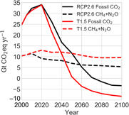
Figure 1. Annual global total fossil CO2 emission scenarios and main non-CO2-GHG emissions (GtCO2eq yr−1). Black continuous and dashed lines—as in RCP2.6 (CLE and MFR); red continuous and dashed lines—as in T1.5 (CLE and MFR) scenarios.
Download figure:
Standard image High-resolution imageHistorical—The historical simulation used the ACCMIP (Emissions for Atmospheric Chemistry and Climate Model Intercomparison Project) aerosol emissions data set for ECHAM runs [40, 41].
RCP2.6-CLE—This experiment uses GHG emissions from RCP2.6 [41], and anthropogenic aerosol (BC, OC and SO4) emissions following the current legislation scenario.
RCP2.6-MFR—As previous experiment, but anthropogenic aerosol emissions follow the maximum feasible reduction scenario.
T1.5-CLE—This experiment uses GHG concentrations from a scenario that was originally developed as one of the sensitivity cases for exploring the 1.5 °C question in Rogelj et al [42]. The scenario is the result of a fully coupled integrated assessment modeling run. The emission budget corresponding to a 50% chance of limiting warming to below 1.5 °C in 2100 in the modeling framework was determined in [42] by doing a few iterations with increasingly stringent emissions budgets. As figure 1 shows, the CO2 emissions in this scenario reach net zero by 2045, about 20 years earlier than in RCP2.6.
T1.5-MFR—As previous experiment, but anthropogenic aerosol emissions follow the maximum feasible reduction scenario.
RCP2.6-2015—This experiment has GHG concentrations as described in RCP2.6 and aerosol forcing frozen at the year-2015 level (from simulation RCP2.6-CLE). It is used as a control case to quantify how large a role the aerosol reductions play in the projected temperature evolution.
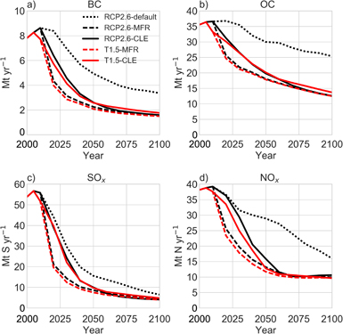
Figure 2. Annual global total anthropogenic aerosol or aerosol precursor emissions of (a) BC, (b) OC, (c) SOx and (d) NOx for the four scenarios. The RCP2.6 emissions (black dotted lines) are presented only for comparison.
Download figure:
Standard image High-resolution imageIn addition to the fossil CO2 emissions, figure 1 also includes the sum of the two main non-CO2-GHG contributors that notably affect climate change and have emissions differing between RCP2.6 and T1.5 scenarios, namely CH4 and N2O, expressed in CO2 equivalent. Although T1.5 scenarios have higher non-CO2-GHG emissions when compared to the RCP2.6 throughout the century, the total CO2 equivalent emissions in T1.5 remain below the level of RCP2.6, making CO2 the dominant driving force (not shown in the figure, for simplicity).
The above anthropogenic aerosol emissions were calculated using the lookup tool supplied by Rogelj et al [43] that provides global air pollution paths consistent with global CO2 emissions. The emissions of different aerosol types from the above listed scenarios are depicted in figure 2. Two distinct patterns in the aerosol emission trends are visible. Firstly, aerosol emissions decline sharply in all scenarios. As many of the anthropogenic aerosol species are to a large extent co-emitted with CO2, the fast reductions in CO2 emissions under both RCP2.6 and T1.5 also have a strong impact on aerosol emissions. In our scenarios, aerosol emissions depend only on the air quality policy chosen (CLE or MFR) and on CO2 emissions, not on the non-CO2-GHG emissions. This is a reasonable assumption as the link between aerosol and non-CO2-GHG emissions is much weaker than that between aerosol and CO2 emissions. Secondly, the chosen air pollution controls also have a significant effect: all aerosol species depicted in figure 2 clearly show lower emissions for the MFR scenarios than the corresponding CLE scenarios and more than twofold lower than the RCP2.6 default emissions. Thus, the impact of aerosol control policies can be expected to have an important role to play especially in the first half of the century before the net CO2 emissions (and hence co-emitted aerosol emissions) become very low.

Figure 3. Time evolution of the global mean temperature increase above pre-industrial levels as estimated by MAGICC (in standard mode) and ECHAM–UVic. The default RCP2.6 temperature evolution (dotted black line in (a) and (b)) is presented in (a) only for comparison.
Download figure:
Standard image High-resolution image3. Results
3.1. Standard temperature projection
Figure 3 compares the global mean surface temperature increase above pre-industrial levels (averaged over 1861–1880) as predicted by MAGICC (standard setup) and by ECHAM–UVic for the scenarios outlined above. In both models, and all scenarios, the temperature increase stays below the 2 °C threshold throughout the century (temperatures 'relative to pre-industrial' are calculated relative to the 1861–1880 base period). In the RCP2.6-CLE and RCP2.6-MFR scenarios, the peak temperature increase, of 1.7 °C and 1.8 °C, is reached in around 2070–2080 in MAGICC and ECHAM–UVic, respectively. In the RCP2.6-default, the temperature increase peaks at 1.6 °C around 2050, followed by a modest decline, never going below 1.5 °C within the present century. On the other hand, under the T1.5 scenarios the global temperature increase peaks around mid-century, and then declines to 1.5 °C in both models. Under both RCP2.6 and T1.5 scenarios the role of the aerosol reduction scenario is small towards the end of the century, which is expected considering that a large majority of the anthropogenic aerosols are co-emitted with CO2, which has net negative emissions by that time. However, the chosen aerosol scenario has a clear impact on the warming rate during the first half of the century. By 2020, in ECHAM–UVic, both the RCP2.6-MFR and T1.5-MFR scenarios lead to higher near-term warming rates, of about 0.35 °C decade−1 (about 0.13 °C decade−1 more than year-2015 aerosol forcing), while the CLE scenarios reach a maximum of 0.26 °C decade−1 by about the same time, showing that, regardless of the aerosol emission scenario applied, the warming is similar time-wise, and is well above the IPCC AR5 projected warming of about 0.2 °C decade−1. Figure 3 also shows that the peak temperature reached under T1.5 depends on the chosen aerosol mitigation scheme. In MAGICC, this peak temperature is 1.75 °C under T1.5-MFR and 1.71 °C under T1.5-CLE. These results highlight that the fast adaptation of very stringent air quality mitigation policies could make global warming in the first half of this century noticeably faster and stronger compared to currently agreed policies.
It is also interesting to note that the highest peak temperature is simulated under the T1.5-MFR scenario—despite the fact that CO2 is reduced much faster in this scenario than under the RCP2.6 scenarios. This somewhat surprising finding is due to a combination of two factors. Firstly, the aerosol forcing decreases rapidly in magnitude (figure 5(a)), because of the fast decline of aerosols co-emitted with CO2 and the stringent aerosol controls in the MFR scenario. Secondly, non-CO2-GHG forcing is higher in T1.5 than in RCP2.6 (figure 5(b)). Hence, the contribution of aerosol forcing reduction suggests that the balance between very ambitious simultaneous air quality and climate targets might need careful consideration.

Figure 4. Time evolution of the global temperature distribution (increase above pre-industrial levels) as estimated by MAGICC in probabilistic/historical constrained setup. The default RCP2.6 temperature evolution (dotted black line in (a) and (b)) is presented only for comparison. In the figures, the black and red lines represent the median, while the dark gray and light gray shadings refer to the 25th–75th percentile and the 17th–83rd percentile, respectively.
Download figure:
Standard image High-resolution image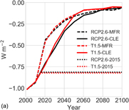
Download figure:
Standard image High-resolution image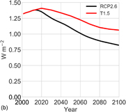
Figure 5. Global mean annual (a) aerosol effective radiative forcing as calculated by ECHAM-HAMMOZ and used in the UVic ESCM runs and (b) forcing by non-CO2 GHGs used in the UVic ESCM runs.
Download figure:
Standard image High-resolution imageFigure 3 also includes two simulations that have aerosol forcing fixed to year-2015 values (RCP2.6-2015 and T1.5-2015). The purpose of these runs is to quantify the role of aerosol reductions on the projected temperature evolution. The lower panel of figure 3 indicates that, according to ECHAM–UVic, total aerosol reductions account for 0.45 °C (the difference between RCP2.6-CLE and RCP2.6-2015) or 0.47 °C (comparison of T1.5-CLE and T1.5-2015) of warming at the end of the century. This is a very significant fraction of the simulated warming and, given the already-realized global warming of 1.03 °C as calculated for 2015, implies that the aerosol reduction alone under these scenarios is enough to push global warming to the 1.5 °C limit. On the other hand, if aerosol emissions could remain at the 2015 level (e.g. through climate engineering measures such as deliberate aerosol injections into the atmosphere) while drastic CO2 reductions are introduced, the 1.5 °C warming target outlined in the Paris agreement could most likely be met.
3.2. Probabilistic temperature projections
Different models can give different climate responses to the same forcings. Our use of two models alleviates this slightly, but it is important to interpret our results as a demonstration of the effects of different air-quality policies rather than exact predictions. However, to explore the uncertainty of the temperature response, we also computed probabilistic time-evolving temperature projections for all five scenarios with MAGICC. The median temperature estimates (lines in figure 4) are about 0.1 °C higher than the global mean temperature estimated with MAGICC in the standard setup (figure 3(a)). The resulting range (66%, that is, between the 17th and 83rd percentiles) of temperature estimates for the RCP2.6 default scenario spreads from 1.41 °C–2.06 °C by 2100, giving likelihoods of 81% and 28% for global temperature increase staying below 2 °C and below 1.5 °C, respectively. The significant aerosol emission reduction scenarios RCP2.6 CLE and RCP2.6 MFR yield temperature ranges of 1.47 °C–2.18 °C and 1.47 °C–2.20 °C, respectively. Both scenarios reduce the likelihood of remaining under 2 °C to 70%, and of under 1.5 °C to 23% in comparison to RCP2.6-default, confirming the warming effect of aerosol emission reduction discussed above. As mentioned above, the original T1.5 scenario, adopted from Rogelj et al [42], was constructed to correspond to a 50% chance of limiting warming to below 1.5 °C in 2100. The additional aerosol emission reduction considered here decreased this percentage to 40% (T1.5-CLE) and 37% (T1.5-MFR). In these scenarios the temperature ranges in 2100 are 1.29 °C–1.95 °C for CLE and 1.31 °C–1.99 °C for MFR, while the likelihood of remaining under 2 °C moved up to 87% and 84%, respectively, in comparison to RCP2.6-default. Based on the analysis of the MAGICC6 results, the RCP2.6 scenarios leading to concentrations of 450–515 ppm CO2eq by the end of the century have less than a 33% probability of maintaining the temperature under 1.5 °C. The T1.5 scenarios on the other hand, reaching levels of 430–465 ppm CO2eq by 2100, have a probability greater than 33% but smaller than 50% of staying below 1.5 °C. Our findings are consistent with the results of the mitigation scenarios presented in the Fifth Assessment Report of the IPCC [44]. A summary of the above key characteristics are presented in table 1.
Table 1. Temperature increase range, probabilities of not exceeding 1.5 °C and 2 °C, and CO2eq concentration range in 2100 as calculated by MAGICC6 with probabilistic setup, for the five scenarios.
| Temperature relative to 1861–1880 | 66% CO2eq concentration range in 2100 (ppm) | |||
|---|---|---|---|---|
| 66% temperature range in 2100 (°C) | Probability of not exceeding 1.5 °C in 2100 (%) | Probability of not exceeding 2 °C in 2100 (%) | ||
| RCP2.6 | 1.41–2.06 | 28.2 | 79.7 | 450–512 |
| RCP2.6-CLE | 1.47–2.18 | 23.2 | 70.7 | 450–515 |
| RCP2.6-MFR | 1.47–2.2 | 23.4 | 69.9 | 450–516 |
| T1.5-CLE | 1.29–1.95 | 39.5 | 87.1 | 430–460 |
| T1.5-MFR | 1.31–1.99 | 36.7 | 84.3 | 430–465 |
3.3. Aerosol radiative forcing
The decline in the magnitude of aerosol forcing from the beginning to the end of the century translates into a large positive forcing for all CLE and MFR scenarios relative to 2000 (figure 5). The globally averaged forcing difference between 2100 and 2000 is 0.96 W m−2 (around 0.75 W m−2 relative to 2015) for CLE and MFR scenarios as computed by the ECHAM–UVic combination. The positive forcing resulting from the decrease in aerosol emissions can have considerable climate implications as it is projected to be about 44% (for RCP2.6-CLE and -MFR) and 64% (for T1.5-CLE and -MFR) of the forcing of CO2 in 2100. Although the projected temperature response to identical decreasing aerosol emissions is similar in both models, MAGICC6 delivers a smaller globally averaged aerosol forcing difference of 0.76 W m−2 for CLE and MFR scenarios relative to year-2000, and 0.56 W m−2 relative to year-2015. This discrepancy, as discussed by Harmsen et al [45], comes from the fact that MAGICC6 shows a very large negative forcing effect, because of strong indirect forcing. It is not possible to have consistent comparisons of the present work with previous studies on the effects of diminishing emissions of aerosols on radiative forcing and climate. However, a qualitative comparison could be attempted as a useful framing exercise. There is a large spread of aerosol radiative forcing values in the literature, which depend on the model used and its settings. The following examples consider only those using the RCP2.6 projections for 2100 relative to 2000. At the lower end, Lamarque et al [46] found an increase in aerosol radiative forcing of 0.57 W m−2 using the CAM5 model, while at the upper end Takemura [47] calculated an increase of 1.96 W m−2 using SPRINTARS. Several other studies resulted in values between these extremes (Gillett and von Salzen [48] obtained 0.7 W m−2 with CanESM2, and Bellouin et al calculated approximately 1 W m−2 using HadGEM2-ES). This large variation indicates that additional multi-model work is needed in order to quantify and properly understand the connection between aerosol emission reduction and corresponding climate responses.

Figure 6. ECHAM–UVic computed spatial distribution of the difference between T1.5-MFR and T1.5-CLE in (a) aerosol radiative forcing and (b) surface temperature in 2021–2030, and in (c) aerosol radiative forcing and (d) surface temperature at the end of the 21st century.
Download figure:
Standard image High-resolution image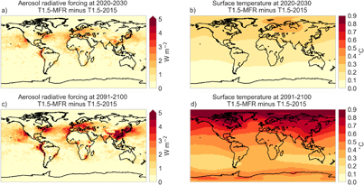
Figure 7. ECHAM–UVic computed spatial distribution of the difference between T1.5-MFR and T1.5-2015 in (a) aerosol radiative forcing and (b) surface temperature in 2021–2030, and in (c) aerosol radiative forcing and (d) surface temperature at the end of the 21st century.
Download figure:
Standard image High-resolution image
3.4. Temperature and aerosol forcing spatial distributions
The differences between the CLE and MFR are also reflected in the surface temperature and aerosol radiative forcing spatial distributions. As the regional pattern is similar in both GHG scenarios, figure 6(a) shows, for simplicity, only the differences between the MFR and CLE cases for the T1.5 scenario averaged over the 2021–2030 period. A decrease in aerosol emissions prescribed by the MFR scenario compared to the CLE scenario averaged over 2021–2030 results in higher temperatures everywhere in the world, predominantly in the Northern Hemisphere where the difference can locally reach 0.3 °C (figure 6(b)). As suggested in several previous studies [49, 50], the Arctic region is more affected than mid-latitudes, partly because of the temperature/albedo feedback and other feedbacks related to the cryosphere. The end of the century shows negligible discrepancy between CLE and MFR scenarios.
The difference between T1.5-MFR and T1.5-2015 climate simulations plotted in figure 7 indicates that the MFR aerosol emission reduction scenario causes a significant regional warming of about 0.2 °C–0.4 °C by 2021–2030 and 0.5 °C–0.9 °C by the end of the century in the Northern Hemisphere. As above, the largest changes occur in the polar regions in connection to changes in snow and ice cover, and are largest over land surfaces compared to ocean surfaces due to the larger thermal inertia of the oceans.
Aerosol forcing decreases in magnitude significantly by 2100, from −1.02 W m−2 in 2000 to −0.06 W m−2 in 2100 in the RCP2.6 scenarios and to −0.05 W m−2 in the T1.5 scenarios. The differences between the CLE and MFR scenarios are largest around year-2020 (0.27 W m−2 for both GHG scenarios). As expected from the aerosol emissions, the aerosol forcings in RCP2.6-MFR and T1.5-MFR are nearly the same, and those in RCP2.6-CLE and T1.5-CLE are also very similar.
The removal of aerosol forcing was most visible in the Northern Hemisphere (figure 7), both in the important emission regions of China, India, Europe, and North America and also in marine regions with significant shipping emissions. A large reduction of aerosol forcing was also simulated in the maritime region in the northwest of South America, a region with an abundance of low clouds susceptible to aerosol emissions. The differences between the MFR and CLE scenarios manifested in these same regions with either high aerosol emissions or high susceptibility to aerosol perturbations.
4. Conclusions
The expected decrease in aerosol emissions during this century in light of growing concerns over the health impacts of air quality ultimately complicates the efforts to moderate climate change. We have shown that reducing aerosol emissions results in a significant warming effect during the first half of the century, predominantly in the Northern Hemisphere. Given that in 2015 we had already experienced a warming of more than 1 °C above pre-industrial levels, the almost 0.5 °C warming from aerosol emission reductions (relative to 2015) would be sufficient to push us to the 1.5 °C limit, even without any additional contribution from GHG emissions. We have also shown that the RCP2.6 scenarios have less than a 33% probability of maintaining the temperature under 1.5 °C, while the same probability for the T1.5 scenarios lies between 33% and 50%. This means that ambitious aerosol mitigation leaves little room for CO2 emissions. Although the global mean temperature increase is held in this study below 2 °C with a probability of well above 66% in all scenarios, the differential warming of land and ocean will cause different regions to warm at higher rates, and the 2 °C threshold to be exceeded in the first half of the century.
When comparing ambitious aerosol emission reduction scenarios (which likely result from ambitious CO2 mitigation), the difference in long-term global mean temperature is negligible, but near-term warming is dependent on the pace of aerosol emission reductions. As such, although beneficial for air quality and human health, the MFR scenario poses a larger threat to climate mitigation than the CLE scenario does, as it could prompt more rapid and magnified warming in the coming years. Unless only the BC-rich emissions are targeted [22], which would lead to less aggravated global warming, the rapid warming due to ambitious aerosol emission reductions should be taken into account and should be treated with caution when creating GHG emission reduction plans to meet the 1.5 °C temperature target.
The results of this study show that moderate aerosol emissions (CLE) and very restrictive, almost unrealistic, GHG emission reductions (such as T1.5) that require a massive scaling up of CO2 removal [51] are needed (but are probably not sufficient) to reach the goal of 1.5 °C warming by 2100—albeit this entails overshooting the 1.5 °C limit (but still remaining under 2 °C) for most of the century. On a more positive, but less healthy, note, the aerosol emissions could be, theoretically, decreased only as would naturally follow from CO2 emission reductions, as they are co-emitted species. The impact of aerosol mitigation scenarios in the context of ambitious CO2 mitigations were found to have a negligible impact on global temperature, a result also supported by a previous study by Rogelj et al [18].
Acknowledgments
This work was supported by the Academy of Finland Center of Excellence program (grant no. 307331). Antti-Ilari Partanen was funded by the Fonds de Recherche du Québec - Nature et technologies (grant number: 200414), Concordia Institute for Water, Energy and Sustainable Systems (CIWESS) and the Academy of Finland (grant number: 308365). The ECHAM-HAMMOZ model was developed by a consortium composed of ETH Zurich, Max Planck Institut für Meteorologie, Forschungszentrum Jülich, the University of Oxford, and the Finnish Meteorological Institute, and managed by the Center for Climate Systems Modeling (C2SM) at ETH Zurich. The UVic ESCM was run through the Compute Canada network at supercomputer Guillimin of McGill University in Montreal, Canada. The authors thank Muzaffer Ege Alper for help with calculating the probabilities of not exceeding 1.5 °C and 2 °C temperature increase thresholds.