

Abstract
The grassland of the Tibetan Plateau forms a globally significant biome, which represents 6% of the world's grasslands and 44% of China's grasslands. However, large uncertainties remain concerning the vegetation carbon storage and turnover time in this biome. In this study, we quantified the pool size of both the aboveground and belowground biomass and turnover time of belowground biomass across the Tibetan Plateau by combining systematic measurements taken from a substantial number of surveys (i.e. 1689 sites for aboveground biomass, 174 sites for belowground biomass) with a machine learning technique (i.e. random forest, RF). Our study demonstrated that the RF model is effective tool for upscaling local biomass observations to the regional scale, and for producing continuous biomass estimates of the Tibetan Plateau. On average, the models estimated 46.57 Tg (1 Tg = 1012g) C of aboveground biomass and 363.71 Tg C of belowground biomass in the Tibetan grasslands covering an area of 1.32 × 10⁶ km2. The turnover time of belowground biomass demonstrated large spatial heterogeneity, with a median turnover time of 4.25 years. Our results also demonstrated large differences in the biomass simulations among the major ecosystem models used for the Tibetan Plateau, largely because of inadequate model parameterization and validation. This study provides a spatially continuous measure of vegetation carbon storage and turnover time, and provides useful information for advancing ecosystem models and improving their performance.
Export citation and abstract BibTeX RIS

Original content from this work may be used under the terms of the Creative Commons Attribution 3.0 licence.
Any further distribution of this work must maintain attribution to the author(s) and the title of the work, journal citation and DOI.
1. Introduction
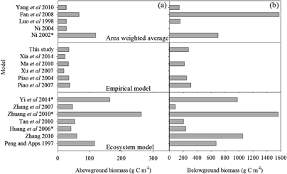
Figure 1. Estimated values of aboveground biomass (a) and belowground biomass (b) of the Qinghai–Tibet Plateau according to different models (Fan et al 2008, Huang et al 2006, Luo et al 1998, Ma et al 2010, Ni 2002, 2004, Peng and Apps 1997, Piao et al 2004, 2007, Tan et al 2010, Xia et al 2014, Xu et al 2007, Yang et al 2010, Yi et al 2014, Zhang 2010, Zhang et al 2007 and Zhuang et al 2010). ⁎ Indicate the studies that did not report belowground biomass, and a ratio between AGB to BGB (0.17) derived from other studies was used to calculate belowground biomass.
Download figure:
Standard image High-resolution imageThe Tibetan Plateau is the highest and largest plateau in the world, with an average elevation that exceeds 4000 m above sea level and covering an area of about 2.5 million km2. During the past several decades, the Tibetan Plateau has become one of the most sensitive regions to rapid climate warming, in that its mean annual temperature has increased by 0.26 °C per decade from 1961–2005, which is twice the global mean temperature change (Lu and Liu 2010, Xu et al 2017). Climate warming has the potential to substantially impact the structure and function of ecosystems, and especially alter the carbon cycle processes (Zhuang et al 2010). Biomass, a key component of the carbon cycle, strongly impacts both net ecosystem production and the carbon budget. Therefore, there is a considerable need to quantify the stocks of carbon that are held within plant communities, as well as the rates at which these stocks are cycled, to improve both predicting and modeling ecosystem carbon dynamics (Richardson et al 2010).
With regard to biomass, turnover time, which refers to the amount of time required for the replacement of biomass in the ecosystem, is a critical parameter in the global carbon cycle (Körner 2000, Saugier et al 2001) and it contributes to the feedback between the terrestrial carbon cycle and the climate (Friend et al 2014). In particular, the biomass turnover time substantially impacts the soil organic carbon on the Tibetan Plateau (Taghizadeh-Toosi et al 2016). This region contains a large amount of soil carbon due to low decomposition rates driven by low temperature (Ding et al 2017). However, the high carbon storage is sensitive to ongoing global warming (Ding et al 2016). Biomass turnover time is highly variable across space and time because it usually is determined jointly by climate, soil, vegetation type (Gill and Jackson 2000). Currently, patterns and determinants of the variability in the turnover time of biomass on the Tibetan Plateau remain poorly understood.
The natural vegetation on the plateau is dominated by alpine grasslands, which cover >60% of its area (Editorial Board of Vegetation Map of China Chinese Academy of Sciences (EBVMC) 2001). Many studies have conducted to evaluate the pool size and spatial variation of grassland biomass on the Tibetan Plateau, but to date, the different methods are inconclusive regarding the magnitude of biomass (figure 1). For example, Zhuang et al (2010) used a terrestrial ecosystem model (TEM) to estimate the aboveground biomass of the Tibetan Plateau at 262.51 g C m−2, which is 13.46 times the estimate of 19.5 g C m−2 reported by Xu et al (2007) (figure 1).
Viable alternative methods to estimate biomass are area-weighted average method, processes-based ecosystem model and empirical model. Area-weighted average method estimated the total biomass by multiplying its surveyed carbon density by the total area, for each grassland type (Ni 2004). This method could only provide the regionally averaged biomass—i.e. by county, province or ecosystem type—as it cannot provide detailed spatial patterns of biomass (Luo et al 2002). Conversely, processes-based ecosystem models are good tools to form mechanistic understandings, but there are still large uncertainties among the processes-based models. For example, the maximum and minimum model estimates of aboveground biomass of Tibetan Plateau ranged sixfold and those of belowground biomass 18-fold (figure 1). Empirical models are based on the relationship between biomass observations and meteorological or remote-sensing variables. These methods also strongly depend on the availability of robust observations.
Currently, as an advanced empirical model, machine learning methods have been increasingly developed for explicitly quantifying biomass regionally, especially through the relationships between remote-sensing variables and biomass (Xia et al 2014). Satellite data provides relatively frequent and spatially contiguous monitoring of surface biophysical variables affecting biomass. Several approaches including artificial neural networks, regression trees, support vector regression, and random forest (RF) have been widely employed to estimate regional biomass and other carbon cycle variables. Machine learning methods are independent on relationships between response variable and predictive variables, especially when compared with traditional empirical models like linear regression that have a requirement of Gaussian distribution for the input variables. In addition, machine learning methods can account for a nonlinear relationship between predictive and target variables and allow both continuous and discrete variables.
Compared to various machine learning methods, the RF algorithm developed by Leo Breiman and Cutler Adele has been regarded as one of the best methods, because it can simulate complex interactions of independent variables and is robust in regard to outliers (Breiman 2001). The RF runs efficiently on large datasets, and can handle thousands of input variables without variable deletion. The RF algorithm has been applied to monitor forest growth, estimate crop production, and classify vegetation type (Mutanga et al 2014, Puissant et al 2014, Wang et al 2016). Recently, several model comparisons showed that RF models produced more accurate estimates of biomass than other machine learning models (Gagliasso et al 2014). In addition, previous studies reported that quantity of observations highly restricted performance of RF model (Rödenbeck et al 2015).
Employing a substantial number of biomass observations offers the best opportunity for accurately estimating biomass and its turnover time on the Tibetan Plateau. More importantly, the increasing observations now available cover a wide range of geographic and climate regions, which is of clear value for upscaling the site-level observations to the region scale. The primary objectives of this paper were: (1) to develop the RF model for estimating aboveground and belowground biomass by using adequate observations, (2) to quantify the aboveground and belowground biomass based on the RF model, and (3) to estimate the turnover time of belowground biomass on the Tibetan Plateau.
2. Data and methods
2.1. Biomass datasets
In this study, we collected three datasets of biomass observations taken on the Tibetan Plateau. In total, in the present study, there were 1689 and 174 observations available for the estimates of aboveground and belowground biomass (figure 2), respectively. The first dataset was from Yang et al (2010), in which the aboveground biomass (AGB) available at stacks.iop.org/ERL/13/014020/mmedia and belowground biomass (BGB) were measured at 115 and 97 sites respectively on the Tibetan Plateau during July and August of 2001–2004. At each site (10 m × 10 m), the AGB was sampled in five plots (each 1 m × 1 m) and the BGB in three soil pits, each consisting of a block of 0.5 m × 0.5 m × actual root depth. Biomass samples were oven-dried at 65 °C to a constant weight.
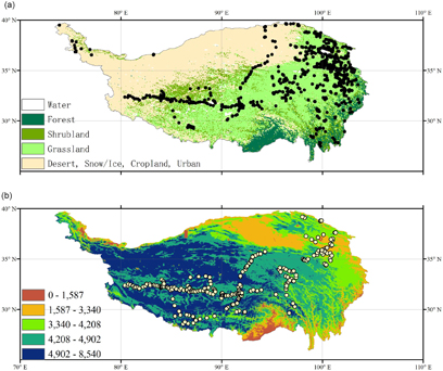
Figure 2. Sampling plots of aboveground biomass (a) and belowground biomass (b). Background maps of (a) and (b) show the land cover type and altitude (in meters above sea level).
Download figure:
Standard image High-resolution imageThe second dataset only included ABG observations taken at 1497 sites on the eastern Qinghai–Tibet Plateau during July and August of 2005–2006 (Feng et al 2011). Each site had a minimum area of 100 m × 100 m and the AGB was sampled in three to five plots (each 1 m × 1 m). All the biomass samples were air-dried, and they were assumed to have 15% water content, which was excluded when they were used for the model development and validation.
The third dataset was derived from a set of field surveys conducted during late July to early August in 2011 and 2012 (Zhu et al 2016). In total, 77 fenced sites were surveyed, and five 1 m × 1 m quadrats were laid out randomly within each 100 m × 100 m site. Both AGB and BGB were sampled and the soils weighed after removing any dead parts and being oven-dried at 65 °C for 72 hours to a constant weight.
2.2. Satellite and climate datasets
Normalized difference vegetation index (NDVI) data were used for two purposes in this study. First, a regional biomass model was developed based on the relationship between biomass measurements and their corresponding NDVI at the sites. Second, the geospatial NDVI data layers were used to calculate the spatial patterns of biomass using the biomass model developed in the present study. Specifically, we used the biweekly NDVI from the Global Inventory Monitoring and Modeling Studies (GIMMS) group as derived from the National Oceanic and Atmospheric Administration's Advanced Very High Resolution Radiometer (NOAA/AVHRR). The AVHRR is the non-stationary NDVI version 3 dataset made available by NASA's GIMMs-3g group (Pinzon and Tucker 2014). This dataset is more commonly referred to as NDVI3g, with the suffix '3g' referring to the third generation processing that was applied to correct for any orbital drift effects, calibration, viewing geometry, stratospheric volcanic aerosols, and other errors that are unrelated to vegetation change. Each 15 day data value is the result of a maximum value composite (Holben 1986), a process that aims to minimize the influence of atmospheric contamination from the aerosols and clouds.
A forcing dataset including the daily temperature, precipitation, relative humidity, daylight hours, and wind speed was used in the present study to develop the model and to estimate the regional biomass (Yuan et al 2014). The thin plate-smoothing splines method was used to generate the daily climate variables throughout all of China at a spatial resolution of 25 km of latitude and longitude (Yuan et al 2015). The fitted trivariate splines incorporated a spatially varying dependence on the ground elevation and were automatically adapted to the large variation in the station density throughout China. The gridded climate dataset was resampled to match the ∼8 km resolution of the NDVI dataset.
2.3. Random forest
RF is a machine learning method for classification and regression. It is a combination of tree predictors, such that each tree depends on the values of a random vector that is sampled independently, with the same distribution for all trees in the forest. Random forest operates by constructing a multitude of decision trees for a given training time and outputting the class that is the mode of the classes (classification) or the mean prediction (regression) of the individual trees. The generalization error for random forest converges to a limit as the number of trees in the forest becomes larger. The first algorithm for the random decision forests was created by Ho (1998) using the random subspace method, which is an extension of the algorithm developed by Breiman (2001). The R package of random forest was used in the present study (randomForest_4.6–12), as modified by Andy Liaw and Matthew Wiener from the original Fortran by Leo Breiman and Adele Cutler (https://cran.r-project.org/web/packages/randomForest).
Table 1. Comparison of the various models used for simulating aboveground and belowground biomass.
| Method | Pred. | R2 | RMSEa | PEb | RPEc |
|---|---|---|---|---|---|
| Aboveground biomass (39.09 g C−2 yr−1)d | |||||
| Random forest | 39.21 | 0.76 | 10.65 | 0.10 | 0.28% |
| NDVI-derived | 40.12 | 0.58 | 19.21 | 1.03 | 2.63% |
| Kriging interpolation | 30.21 | 0.23 | 21.92 | −8.88 | −22.71% |
| Natural neighbor interpolation | 25.98 | 0.19 | 24.32 | −13.11 | −33.54% |
| Thin-plate spline | 26.89 | 0.31 | 23.41 | −12.20 | −31.21% |
| Belowground biomass (243 g C m−2 yr−1)e | |||||
| Random forest | 239.53 | 0.64 | 98.42 | −3.50 | 1.44% |
| AGB-derived | 214.32 | 0.25 | 198.22 | −28.68 | −11.80% |
| Kriging interpolation | 192.39 | 0.15 | 201.25 | −50.61 | −20.82% |
| Natural neighbor interpolation | 182.31 | 0.06 | 212.37 | −60.69 | −24.97% |
| Thin-plate spline | 201.23 | 0.16 | 219.32 | −41.77 | −17.19% |
aRoot mean squared error. bAbsolute predictive error. cRelative predictive error. d,eIndicate observed mean values of aboveground and belowground biomass.
We developed a predictive AGB and BGB model using RF. The explanatory variables included mean air temperature, maximum air temperature, minimum air temperature, precipitation, relative humidity, solar radiation, standardised precipitation–evapotranspiration index (SPEI) and NDVI by year and by the four seasons (i.e. winter, spring, summer, and autumn)—for a total of 40 variables. For predicting BGB, the AGB also is used as an explanatory variable. In addition to the full model that included all 40 and 41 independent variables for AGB and BGB respectively, we also developed a subseries of models by dropping one or more variables at a time. To select the best model, we evaluated the performance of each model based on their root mean squared error (RMSE). For each model, 80% of the observations are selected randomly for training, leaving 20% for validation, and the model is run 1000 times or reaches all combinations of observations. A free R-package was used to calculate SPEI on the Tibetan Plateau (Vicente-Serrano et al 2010) (http://spei.csic.es/tools.html).
We also applied other common methods to estimate both the AGB and BGB and compared these with the RF-based model (table 1). The NDVI-derived exponential equations (NDVI-derived method) were used to estimate the aboveground biomass as follows:

where a and b are the coefficients. For belowground biomass, the approach of the aboveground vs belowground biomass relationship has been the most common way to estimate belowground biomass at different scales, from the local to the landscape, region, and biome (Mokany et al 2006). Piao et al (2007) used the fixed ratio between aboveground and belowground biomass as derived from the observations, while Ma et al (2010) used a linear relationship to estimate the belowground biomass. Our study uses the linear relationship between AGB and BGB (AGB-derived method) as follows:

where α and β were undetermined coefficients. Moreover, three spatial interpolation methods also were used: kriging, natural neighbor, and thin-plate spline. The former two were performed in ArcGIS v.9.3 (ERSI Inc.), while the latter was implemented using the ANUSPLIN package following Yuan et al (2015). As with the RF models, 80% of observations were selected randomly for calibration with the remainder used for validation, and the model was run 1000 times to complete the cross-validation.
2.4. Turnover time
The longevity of aboveground parts in grassland is 1 year; hence, this study only calculated the turnover time (TR) of belowground biomass. Because the biomass was measured during July and August, when the aboveground biomass is at its maximum over the entire year, we considered that the AGB was equal to aboveground net primary production (ANPP). Our study calculated belowground turnover time at given grid cell i as:

where the coefficient value of 0.5 was used to calculate the NPP from the gross primary production (GPP). In this study, we used the averaged GPP derived from EC-LUE model (Yuan et al 2007, Yuan et al 2010, Yuan et al 2014) and MODIS-GPP product (Running et al 2004).
3. Results
Based on the AGB and BGB observations, we tested the model's performance on all possible combinations of the explanatory variables (see above). Annual precipitation, summer NDVI, and summer relative humidity were found to be the best combinations for simulating AGB, while summer NDVI, annual air temperature, and summer SPEI were selected for simulating BGB. We then validated the model in the spatial domain using a cross-validation. The cross-validation showed that the models explained 76% and 64% of AGB and BGB over all measurements respectively (figure 3), and that the performance of AGB was better than that of BGB.

Figure 3. Observed and estimated aboveground biomass (a) and belowground biomass (b). The dashed lines indicate a 1:1 correspondence and the solid lines are the fitted linear regressions to the data.
Download figure:
Standard image High-resolution image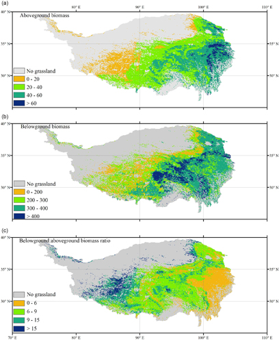
Figure 4. Regional patterns of aboveground biomass ((a), unit: g C m−2), belowground biomass ((b), unit: g C m−2) averaged from 1982–2010, and belowground:aboveground biomass ratio (c).
Download figure:
Standard image High-resolution image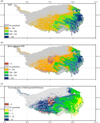
Figure 5. Spatial patterns of net primary production (NPP, unit: g C m−2 yr−1) (a), belowground NPP ((b), unit: g C m−2 yr−1), and the turnover time of belowground biomass ((c), unit: yr).
Download figure:
Standard image High-resolution image
Figure 6. Relationships between the turnover time of belowground biomass and annual precipitation (a), NDVI (b), and mean annual temperature (c). The data of turnover time > 50 years (12% of entire data) were not included in this figure. The color bar indicates the density of points in the scatter plot.
Download figure:
Standard image High-resolution image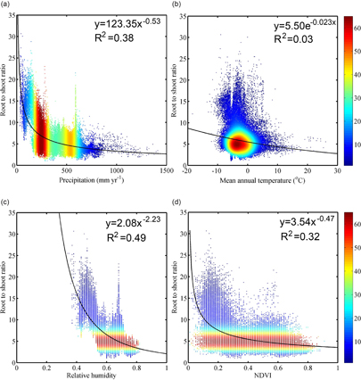
Figure 7. Relationships of the ratio of belowground biomass and aboveground biomass (%) with annual precipitation (a), mean annual temperature (b), relative humidity (c) and NDVI (d). The color bar indicates the density of points in the scatter plot.
Download figure:
Standard image High-resolution image
Figure 4 showed the spatial distribution of the average values of AGB and BGB as predicted by the random forest model in our study. The overall mean AGB and BGB on the Tibetan Plateau were 35.28 g C m−2 and 275.11 g C m−2, respectively. We then summed total biomass for the entire plateau and obtained the estimates of 46.57 Tg C and 363.71 Tg C for AGB and BGB, respectively. Both the AGB and BGB declined from the southeastern to the northwestern part of the plateau (figure 4), corresponding well to the precipitation gradient across the plateau.
The turnover time of belowground biomass showed substantial spatial heterogeneity on the Tibetan Plateau. The median turnover time was 4.25 years, and it ranged from 0.28–143.69 years. The longest turnover time occurred over the western part of the plateau characterized by low temperature and precipitation, and the turnover time decreases with temperature and precipitation (figure 5(c); figure 6).
4. Discussion
4.1. Estimates of aboveground and belowground biomass
This study combined three, large-scale comprehensive sets of observations of biomass on the Tibetan Plateau (1689 aboveground biomass and 174 belowground biomass observations). Based on a RF model, we upscaled these site-level measurements to arrive at estimates of regional-scale biomass. Our results demonstrated that in combination with other satellite-derived and climatic variables, the random forest displayed a good performance for predicting both the AGB and BGB, as confirmed by the cross-validation (figure 3). Often the performance of the data-driven method is highly restricted by the quantity of training datasets (Chen et al 2014). Our current estimates greatly benefited from the sufficient observations, especially for aboveground biomass, and these observations covered the major geographical and climate regions of the Tibetan Plateau.
Our study provides a new biomass estimate of Tibetan Plateau and offers an opportunity to bridge the gap between sparse data and correct parameterization of future ecosystem models. Figure 1 showed larger inter-model differences among process-based models relative to the area-weighted average methods and empirical models. These results were unexpected because the process-based models were developed by integrating mechanistic processes and have been evaluated by using the observations of Tibetan Plateau. Therefore, they were supposed to represent relatively similar and consistent regional biomass simulations. These results imply that model need be evaluated over the regional scales against defined references (i.e. benchmarks) that can be used to diagnose the model's strengths and deficiencies for future improvement. Undoubtedly, ecosystem models must attempt to better characterize the spatial and temporal heterogeneity of ecosystem processes and pursue further validation against observations (Baldocchi et al 1996, Friend et al 2007, Yuan et al 2010). To reliably simulate the dynamics of biomass, the models should accurately reproduce the relevant key ecosystem processes, namely vegetation primary production, carbon allocation, and turnover time. Based on the random forest model, our estimates will be useful for evaluating model as a benchmark.
Previous studies have used a satellite-based vegetation index to upscale the site observations to estimate levels of regional aboveground biomass using either linear or exponential equations (Piao et al 2004, 2007, Ma et al 2010, Xia et al 2014). The present study demonstrated that random forest showed better performance than the NDVI-derived approach that was frequently used for estimating regional carbon budgets (higher R2 and smaller RMSE, table 1). Basically, as a machine learning technique, random forest can develop multivariate models that indicate both linear and nonlinear relationships (Smirniotis 2013) that usually occur when simulating biomass based on biotic and climatic properties (Chapin et al 2001). By comparing all combinations of all variables, the best combinations of variables could thus be selected to estimate the biomass and not only include NDVI. Although our estimates were close to previous estimates regarding to averaged biomass over the entire Tibetan Plateau (figure 1), but there were large differences of spatial patterns (data not shown).
For the belowground biomass estimates, our results indicated the better performance of the random forest model (table 1). Notably, the three GIS interpolation methods showed the poorest performance due to a strong reliance on observations. However, due to the extensive labor and efforts to acquire them, there is large imbalance in the geographic distribution of belowground biomass observations (figure 2(b)). Previous studies have highlighted that statistical models are confined to the data dimensions (e.g. space, time, climate, environmental behavior) in which they are trained; thus, extrapolating outside those dimensions may not be robust and may lead to large uncertainties (Chen et al 2014). In addition, empirical models often used the relationship or ratio between AGB and BGB to estimate the latter (Piao et al 2007, Ma et al 2010). However, numerous studies have reported large heterogeneities of ratio between AGB and BGB over the precipitation and temperature gradients (Yang et al 2010).
It should be noticed that the performance of AGB model was much better than that for BGB (figure 3). Compared with the aboveground plant components, there are complex physiological processes that collectively determine root biomass in a given region and time (Chapin et al 2001). In general, the lifespan of a leaf is less than 1 year, but that of a root will often exceed 1 year (Gill and Jackson 2000). Therefore, various environmental variables and cumulative effects will substantially impact the belowground biomass. Moreover, a satellite-based vegetation index can directly indicate the condition of aboveground plants components, but to date, none of variables can directly characterize the belowground components, which substantially limits our ability to simulate belowground biomass dynamics. Because of the greater effort involved in measuring belowground biomass (Clark et al 2001), it is measured less extensively, and thus with greater error, than is aboveground biomass. In addition, it should be noticed that the belowground biomass was underestimated at the large belowground biomass regions. The uncertainty of belowground biomass measurement probably is one of the most causes for underestimations. It is challenged to distinguish the live and dead roots, therefore the belowground biomass probably was over measured.
Ratio between BGB and AGB (R:S) in terrestrial ecosystems is partly determined by climatic factors (Hui and Jackson 2005). Our results showed the significant decreased trends of R:S along the gradients of precipitation and relative humidity (figures 7(a) and (c)). These trends were consistent with those of other findings globally. At the global scale, Mokany et al (2006) demonstrated that R:S in grasslands significantly decreased with increases in annual precipitation. In this study, the weak correlation between mean annual temperature and R:S was observed (figure 7(b)), which implied the dominated role of precipitation on the Tibetan Plateau.
4.2. Spatial pattern of biomass turnover time and environmental regulations
Roots constitute a vital interface between plants and soils and thus play a crucial role in driving the carbon, nutrient, and water cycles of an ecosystem. Their continuous growth and dieback, often termed root turnover, may constitute a major carbon input to the soils and thus significantly contribute to the belowground carbon cycle. For this reason, it important to accurately estimate not only the standing biomass of roots but also their turnover time. A great deal of scientific effort has been made to quantify turnover times (Gill and Jackson 2000), and although the methods have gradually improved, it is still one of the most difficult ecosystem characteristics to accurately describe and quantify (Lukac 2012). Almost all of the ecosystem models assume that the turnover time of the root system is a constant; this implies that for all grasses the proportion of roots that die annually is invariant (De Kauwe et al 2014). However, numerous studies have shown the large spatial variation in the actual turnover times of roots (Carvalhais et al 2014). Our model estimates point to high spatial heterogeneity in root turnover time, which was supported in the previous conclusion (figure 6).
The results showed a shorter turnover time of the belowground biomass with greater precipitation and temperature (figure 6), which is consistent with previous studies (Gill and Jackson 2000, Carvalhais et al 2014). There are two plausible causes for the decreasing trend of turnover time with higher temperature and precipitation. First, the maintenance of respiration of the root increases with temperature, such that the optimal lifespan for a root decreases, thus requiring a lower root turnover time (i.e. higher turnover rate) in warmer climates (Gill and Jackson 2000). Second, nitrogen mineralization will increase as the temperature and precipitation increases, which should accelerate plant autotrophic respiration and thus lead to a shorter turnover time (Burton et al 2002). Moreover, new roots have a higher efficiency of absorbing nutrients and water; therefore, plants will accelerate the growth of their roots via a shorter turnover time (Johnson et al 2000, Majdi 2001).
To date, no direct and reliable method of measuring fine root turnover exists. The main reason for this is that the two component processes of root turnover—namely growth and dieback of roots—nearly always happen at the same place and at the same time (Joslin and Wolfe 1999, Gaudinski et al 2001). Further, the estimation of root turnover is complicated by the inaccessibility of the tree root systems and the intensive labour required to sample them, which is often further compounded by site-specific effects created by local soil disturbance (Lukac 2012). Nonetheless, the present study developed a modeling methodology that could be used in the future for the spatially-explicit estimation of root turnover time. Our results demonstrate that biomass measurements, when coupled with vegetation production simulations via machine learning techniques, yields an effective method to estimate the turnover time of roots in the grassland ecosystem. We propose that this approach could be applied to other regions around the world.
In this study, we estimated root turnover time by combining simulations of AGB, BGB, and GPP, and so the model errors will carry over into the turnover time estimates. Over the entire study region, the model estimated a negative BNPP (i.e. NPP (0.5 × GPP) minus AGB) for 7.9% of the sites, mostly distributed on the western plateau with low precipitation and temperature (figure 5(b)). These abnormal simulations occur at the small areas, but which suggest the need to improve our estimates in the future. Previous study also showed that the current satellite-based models tended to underestimate vegetation production (Yuan et al 2014). In addition, the spatial constant ratio of 0.5 was used to simulate NPP from GPP, assuming an invariable ratio of autotrophic respiration with GPP. However, previous studies have reported that the NPP/GPP ratio decreased with increased precipitation, yet it remains unchanged in areas where the water availability is in surplus (Zhang et al 2009). Our study used a constant NPP/GPP ratio to estimate NPP, and thus we likely underestimated NPP for sites with dry conditions.
Our estimates are useful for parameterization of ecosystem models on the Tibetan Plateau. Large uncertainties of biomass estimates were found among the major ecosystem models used before (figure 1). Biomass estimates strongly depend on other carbon cycle variables, such as vegetation production, carbon allocation, and turnover time (Ise et al 2010, McMurtrie and Dewar 2013, Xia et al 2015). Our prior studies revealed large differences in GPP simulations among the ecosystem models for the Tibetan Plateau (Yuan et al 2014), which can strongly impact the biomass estimates (Yuan et al 2010). Moreover, biomass also is important for simulating other carbon cycle variables (i.e. net ecosystem production, soil carbon content). Therefore, a robust estimate of biomass is an important reference point for examining the performance of any ecosystem model, and likewise provides a practical reference point for separating the model errors. Finally, the estimated turnover time of belowground biomass could be directly integrated into the ecosystem models to improve their performance.
5. Summary
The magnitude and turnover time of biomass are crucial estimates for projecting the terrestrial carbon budget. Based on a substantial number of field surveys, this study used a machine learning method (i.e, random forest, RF) to develop a data-derived model for predicting both aboveground and belowground biomass. The results show that the RF enables the adequate retrieval of the regional pattern of biomass on the Tibetan Plateau. Over the entire Tibetan Plateau, the estimated aboveground and belowground biomass were 46.57 Tg C and 363.71 Tg C. Moreover, by combining the vegetation production and carbon allocation coefficients with biomass estimates, the turnover time of belowground biomass was estimated for the Tibetan Plateau. The results show the belowground biomass turnover time is spatially heterogeneous, with a median turnover time of 4.25 years, and dominated by temperature and precipitation influences. Our study thus provides the new data for the biomass and its turnover time on the Tibetan Plateau, which should be useful for advancing ecosystem models and their parameterization and validation.
Acknowledgments
The research is supported by the National Key Project (2016YFA0602701), General Program of National Natural Science Foundation of China (31570468), One Hundred Person Project of Chinese Academy of Sciences (Y329k71002), Youth Changjiang Scholars Programme of China (Q2016161) and National Youth Top-notch Talent Support Program.