

Abstract
Climate change impacts on water availability and hydrological extremes are major concerns as regards the Sustainable Development Goals. Impacts on hydrology are normally investigated as part of a modelling chain, in which climate projections from multiple climate models are used as inputs to multiple impact models, under different greenhouse gas emissions scenarios, which result in different amounts of global temperature rise. While the goal is generally to investigate the relevance of changes in climate for the water cycle, water resources or hydrological extremes, it is often the case that variations in other components of the model chain obscure the effect of climate scenario variation. This is particularly important when assessing the impacts of relatively lower magnitudes of global warming, such as those associated with the aspirational goals of the Paris Agreement.
In our study, we use ANOVA (analyses of variance) to allocate and quantify the main sources of uncertainty in the hydrological impact modelling chain. In turn we determine the statistical significance of different sources of uncertainty. We achieve this by using a set of five climate models and up to 13 hydrological models, for nine large scale river basins across the globe, under four emissions scenarios. The impact variable we consider in our analysis is daily river discharge. We analyze overall water availability and flow regime, including seasonality, high flows and low flows. Scaling effects are investigated by separately looking at discharge generated by global and regional hydrological models respectively. Finally, we compare our results with other recently published studies.
We find that small differences in global temperature rise associated with some emissions scenarios have mostly significant impacts on river discharge—however, climate model related uncertainty is so large that it obscures the sensitivity of the hydrological system.
Export citation and abstract BibTeX RIS

Original content from this work may be used under the terms of the Creative Commons Attribution 3.0 licence.
Any further distribution of this work must maintain attribution to the author(s) and the title of the work, journal citation and DOI.
1. Introduction
The hydrological cycle is an essential part of the climate system and therefore very sensitive to climate variability and changes. Small, sometimes insignificant variations in climate often lead to significant changes in hydrological processes (Hattermann et al 2011). Generally, it is expected that an increase in temperature will intensify the hydrological cycle (Kundzewicz and Schellnhuber 2004), but the feedback is nonlinear because different climate variables may have opposing effects on specific components of the water cycle. Increases in temperature and radiation, for example, stimulate evapotranspiration and may lead to lower water availability in a certain region, while increases in precipitation without notable changes in evapotranspiration would increase water availability.
Important for the water cycle is how climate trends manifest in a certain region or river basin. Moreover, in large scale river basins, it might be that opposing trends in climate will develop in headwaters and lowlands, i.e. increases in precipitation in upstream parts may result in higher discharge while precipitation downstream may even decrease. The Nile basin shows such opposing trends, with increases in projected precipitation in the headwaters of the Blue and White Nile and decreases downstream (Teklesadik et al 2017, Liersch et al 2016). Mishra et al (2017) found that evapotranspiration will increase under scenario conditions in all seven large scale basins they investigated, among them the Blue Nile, but this increase is compensated by an increase in precipitation in five out of seven river basins.
The high sensitivity of hydrological processes to climate variability and change increases the demand for the accuracy of climate simulations at the regional scale. In an 'ideal model world', assessments of climate change impacts on natural resources and processes would be only determined by the scenario settings and not by climate and impact models which are needed to translate the scenarios into impacts. However, while there is not much disagreement in temperature increases simulated by different global climate models (GCMs) under specific scenario conditions, more variability and uncertainty exists in projected precipitation trends (IPCC 2013). When analyzing the most recent climate scenario data as delivered by the Coupled (climate) Model Intercomparison Project (CMIP5, Taylor et al 2012) for the Representative Concentration Pathway 8.5 (RCP8.5, van Vuuren et al 2011), the results show that only in 35.4% of the land surface area at least 80% of the precipitation projections agree in the trend direction (see figure 1). Many of the world's largest river basins are located in regions where the precipitation trends do not agree in general or show opposing trends in their total catchment area, for example the Nile, the Niger, the Mississippi or the Amazon.

Figure 1. Mean trend in annual precipitation until end of this century under RCP8.5 scenario conditions (2010–2099, using linear regression of the annual sums) of 18 global climate model results of the Coupled (climate) Model Intercomparison Project (CMIP5). Shaded areas indicate where at least 80% of the model ensemble agrees in the direction of the trend. The red polygons show the locations of the river basins considered in this study (1–Upper Mississippi, 2–Upper Amazon, 3–Rhine, 4–Upper Niger, 5–Blue Nile, 6–Ganges, 7–Upper Yangtze, 8–Upper Yellow, 9–Lena).
Download figure:
Standard image High-resolution imageIn this study, we make use of climate and impact data provided in the framework of the Inter-Sectoral Impact Model Intercomparison Project (ISIMIP, Schellnhuber et al 2014, Warszawski et al 2014). ISIMIP is a community-driven modelling effort bringing together impact modelers across sectors and scales to create consistent and comprehensive projections of the impacts at different levels of global warming, based on the RCPs and Shared Socio-Economic Pathways (SSPs) scenarios (IPCC 2013). The rationale behind ISIMIP is to use ensembles of impact models to find robust trends and to identify the demand for further impact model development. The ISIMIP initiative has boosted a series of publications dedicated to multi-model inter-comparison of climate change impacts. While a first set of hydrology-related publications described global scale impacts (Schewe et al 2014, Dankers et al 2014, Prudhomme et al 2014, Haddeland et al 2014, Davie et al 2013, Wada et al 2013 and Portmann et al 2014), a second set of studies focused on impacts on the hydrological cycle, water resources, seasonality and extremes at the regional scale (e.g. Eisner et al 2017, Vetter et al 2017, Samaniego et al 2017, Mishra et al 2017, Pechlivanidis et al 2017, Wang et al 2017, Gelfan et al 2017, Teklesadik et al 2017 and Su Buda et al 2017). Cross-scale studies using both, the outcomes of global and regional hydrological models, were published in Hattermann et al (2017) and Gosling et al (2017).
The total uncertainty in projected water availability has been investigated to some extent in most of these studies. Climate impacts on seasonal dynamics and quantification of uncertainties, for example, can be found in Eisner et al (2017). Pechlivanidis et al (2017) reported that results are generally more uncertain in dry basins than in wet ones. This finding is supported by Samaniego et al (2017), who also discovered generally a higher contribution of hydrological model uncertainty to total uncertainty in projected droughts (although still being lower than the share of climate model uncertainty). Vetter et al (2017) used ANOVA (analysis of variance) to allocate sources of uncertainty for trends in river discharge in 12 basins using regional scale hydrological data, finding that GCMs contribute the largest uncertainty, but the absolute contribution may vary over the year. Other applications of ANOVA in climate impact analysis can be found in Vidal et al 2016, Giuntoli et al 2015 and Bosshard et al 2013.
One main outcome of these studies is that GCMs contribute in most cases the highest share to the overall impact uncertainty. This is very crucial when looking at the Paris Agreement under the United Nations Framework Convention on Climate Change (hereinafter referred to as 'the Paris Agreement'), which demands for aggregated emission pathways consistent with keeping the increase in the global average temperature to well below 2 °C above pre-industrial levels and pursuing efforts to limit the temperature increase to 1.5 °C. While these seemingly small differences in temperature increase will definitely have a strong effect in specific regions and ecosystems (the most prominent ones possibly being small islands and coral reefs, Frieler et al 2013), many previous studies have shown that the impact of such small temperature differences is not so clear when looking at water resources and hydrological processes (Vetter et al 2015, Hattermann et al 2015, Donnelly et al 2017). As a result, one may ask whether we have the right tools to quantify impacts of such small differences in scenario projections. Therefore, the aim of this study is (a) to systematically allocate and quantify the main sources of uncertainty in the entire model and scenario chain comparing effects of scenarios with small temperature differences and effects of scenarios with strong temperature differences, (b) to analyze and quantify how significant variations in boundary conditions are, (c) to look at scale effects caused by the impact models and (d) to discuss the results in the light of other recent publications and the Paris Agreement.
2. Data and models
In total, daily outputs of up to nine regional and four global hydrological models driven by climate simulations from five GCMs and for four RCP scenarios, for nine large scale river basins have been used. The river basins are shown in figure 1. For some rivers we consider the upper parts only because these are less influenced by human regulation. Table 1 lists the main characteristics of the river basins considered and the hydrological models (HMs) applied (not all regional HMs have been applied to all river basins).
Table 1. Characteristics of the case study basins (drainage area, average air temperature and average annual precipitation for the period 1971–2000) and an overview of the regional and global HM applications in the study (X X indicates application of the same model by two different teams with different model parametrization).
| Basin | Rhine | Niger | Blue Nile | Ganges | Yellow | Yangtze | Lena | Mississippi | Amazon |
|---|---|---|---|---|---|---|---|---|---|
| Gauge | Lobith | Koulikoro | El Deim | Farakka | Tangnaiha | Cuntan | Stolb | Alton | SP Olivenca |
| Drainage area [km2] | 160 800 | 120 000 | 238 977 | 835 000 | 121 000 | 804 859 | 2 460 000 | 444 185 | 990 781 |
| Average T [°C] | 8.7 | 26.5 | 19.4 | 21.1 | −2 | 6.8 | −10.2 | 7.3 | 1.7 |
| Average P [mm yr−1] | 1 038 | 1 495 | 1 405 | 1 173 | 506 | 768 | 384 | 967 | 2 122 |
| Regional models | |||||||||
| ECOMAG | X | ||||||||
| HBV | X X | X | X | X | X | X | X | X | |
| HYMOD | X X | X | X X | X | X X | X | |||
| HYPE | X | X | X | ||||||
| mHM | X | X | X | X | X | X | X | ||
| SWAT | X | X | X | X | X | ||||
| SWIM | X | X | X | X | X | X | X | X | X |
| VIC | X | X | X | X | X | X | X | X | X |
| WaterGAP3 | X | X | X | X | X | X | X | X | |
| Global models | |||||||||
| H08 | X | X | X | X | X | X | X | X | X |
| MPI-HM | X | X | X | X | X | X | X | X | X |
| PCR-GLOBWB | X | X | X | X | X | X | X | X | X |
| WBM | X | X | X | X | X | X | X | X | X |
All models simulate the full water cycle (evapotranspiration, infiltration, generation of runoff and routing of the locally generated runoff along the river network to the outlet), using different spatial disaggregation schemes, with daily precipitation and temperature as main inputs. Global HMs, as defined in our study, operate at the global scale, using globally available input data and their parameters take single values with an assumption that they are applicable everywhere, i.e. they are spatially generalized. Regional HMs in our study are applied to river basins and there has been specific local tuning to get the predictive performance to a high level. While the global models consistently simulate hydrological processes and river routing with a spatial resolution of 0.5°, different approaches for spatial disaggregation are used by the regional models: regular grids (e.g. mHM, VIC and WaterGAP3) and disaggregation schemes with subbasins and hydrological response units (SWIM, HBV, HYPE and SWAT). More information on basic processes represented in the models and input data can be found in Hattermann et al (2017) and with a focus on the regional models in Krysanova and Hattermann (2017) and their calibration and validation in Huang et al (2017).
The river basins were chosen in such a way that they represent important climate regimes: two of them are located in temperate climates (Upper Mississippi and Rhine), one in a subarctic climate (Lena), four in monsoonal type of climates (Ganges, Upper Amazon, Upper Niger, Blue Nile) and two in a continental plateau climate (Upper Yellow and Upper Yangtze). Annual precipitation totals range from lower than 400 mm in the Lena to more than 2000 mm in the Upper Amazon, and mean annual temperature ranges from −10 °C in the Lena to more than 26 °C in the Upper Niger.
All hydrological models used in this study have been driven by the same CMIP5 climate scenario data as provided by ISIMIP. Results of 5 global climate models (HadGEM2-ES, IPSL-CM5A-LR, MIROC-ESM-CHEM, GFDL-ESM2M, NorESM1-M) have been bias corrected by Hempel et al (2013) against global WATCH Forcing Data (WFD, Weedon et al 2011) using a trend-preserving method. The resulting bias-corrected scenario data are daily, 0.5 by 0.5 degrees gridded meteorological forcing data covering the time period 1958–2099. For more information about the climate scenario simulations for the individual river basins including statistics about their projected climate, see Krysanova and Hattermann (2017). A comparison of the performance of the hydrological models from both scales under current climate conditions and impacts under climate scenarios is given in Hattermann et al (2017) and Gosling et al (2017).
3. Methodology
3.1. River discharge
We use river discharge at the outlet of the basins to investigate impact uncertainty. The locations are given in table 1. Considered are mean flows (Q50, the long-term mean daily flow), high flows (Q10, where 10% of the long-term mean daily flows are above this value) and low flows (Q90, 90% of the long-term mean daily flows are above this value). The changes in discharge analyzed in the ANOVA setting are the differences of the monthly or annual mean flows of the years 1971–2000 (reference period) and 2070–2099 (scenario period).
3.2. Total uncertainty of results
The coefficient of variation (cv) of the projected changes in river discharge, modelled by the hydrological models, at the basin outlet is applied as a measure to show the total uncertainty of impacts for each basin. When calculating how cv evolves with time, we apply a 30 year moving window in order to smooth the huge inter-annual variability. Thus, the number of input data to calculate it for each running year is the product of the number of GCMs and HMs applied for each basin multiplied by the 30 annual values.
3.3. ANOVA
We make use of ANOVA to allocate the main sources of uncertainty, because it allows in addition to quantify the significance of variations in the impact chain. ANOVA is a specific form of statistical hypothesis testing for more than two groups. The null hypothesis is that all groups are simply random samples of the same population. ANOVA can be applied to decompose the observed variance in a particular variable into components, which are attributable to different sources of variation (Von Storch and Zwiers 1999). Another main application field is comparing and testing whether or not the means of several groups are equal and thereby quantifying the significance of any source of variation. The sources of variation are blocked into three groups, which are the GCMs, HMs and RCPs (three-way ANOVA). These groups are called factors, and the members of each group are called different factor levels. By variation of the factors we get different responses (in our case river discharge) that we use to quantify sources of uncertainty and the significance of variation of the factors.
3.3.1. Quantification of sources of uncertainty
In ANOVA, the total sum of squares (SST, the squared terms being deviations of single values from the grand mean) is used to express the total variation that can be attributed to the various factors. The three factors used for variance decomposition are the GCMs, HMs and RCPs:
where Yijk is the specific value corresponding to the climate model i, hydrological model j and RCP k, respectively, and  is the overall mean. SST can be further split into three main effects (SSGCM, SSHM, and SSRCP, the squared deviations of single values from their appropriate factor mean), which are effects directly attributable to GCMs, HMs and RCPs, and into four interaction terms (SSGCM⁎HM, SSGCM⁎RCP, SSHM⁎RCP, and SSGCM⁎HM⁎RCP):
The latter are related to non-additive and/ or nonlinear effects (Vetter et al 2015). The equations to calculate main effects, first interaction and second order interaction are given exemplarily in equations (A1−A3) of the appendix.
3.3.2. Significance of variation
The F-test is used for determining the significance of any variation in the factors GCMs, HMs and RCPs. The null-hypothesis is that all variations in different factors have the same effect. The F-test is recommended as a practical test, because of its robustness against many alternative distributions. We have analyzed the distributions of the residuals in all cases and have found no notable deviations from the normal distribution.
In ANOVA, factors can be treated either as being fixed or random. A factor is fixed when the levels under study (the specific GCMs, HMs and RCPs) are the only ones of interest, and in this case any conclusion applies only to this specific setting and no general assumptions beyond this sample can be drawn. A factor can be treated as being random when the levels under study are considered as being random samples from a larger population (of GCMs etc.), and in this case, general conclusions about the larger population (e.g. of GCMs or HMs) are possible. However, because one concludes from a smaller selection to a larger population in the latter case, the discriminative power and thus the significance of the outcome is lower. In our study, we apply ANOVA in the fixed factor mode.
4. Results
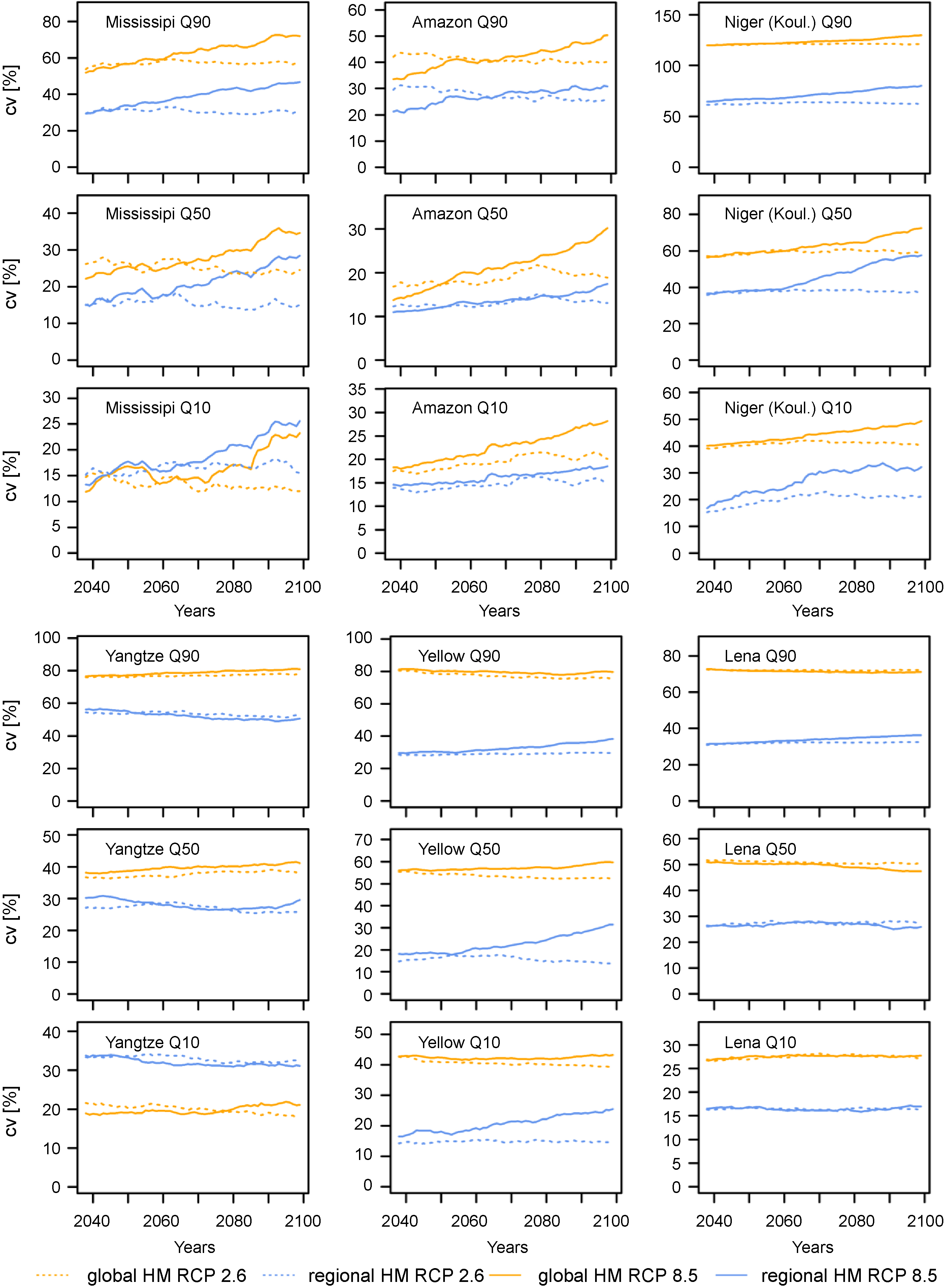
The projected total uncertainty in impacts (changes in river discharge) transient until the end of the century (2070–2099) compared to the reference period (1971–2000) is shown in figure 2 (for the rivers Rhine, Blue Nile and Ganges) and in figure A1 in the appendix (for the rest of the basins), using cv as a relative measure to investigate the development of total uncertainty over time for each river basin and separately for RCPs 2.6 and 8.5. The indicators considered are mean flows (Q50), high flows (Q10) and low flows (Q90) simulated by the global and regional HMs. The results illustrate that the total uncertainty in impacts is increasing under RCP8.5 scenario conditions in most cases until the end of this century. Under RCP2.6 scenario conditions, the uncertainty does not show such a trend in most cases. The strongest increase in impact uncertainty under RCP8.5 is visible in figure 2 for all flows in the Rhine and the Blue Nile with a notable exception, Q90 modelled by global HMs.
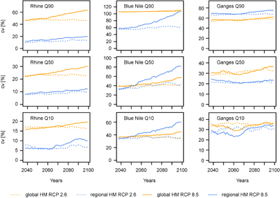
Figure 2. Variability in changes in Q50 (mean flow), Q90 (low flow) and Q10 (high flow) based on all simulation results for the scenarios RCPs 2.6 and 8.5, separately for the regional and global hydrological models (blue and orange curves) for the Lena, Blue Nile and Ganges in the period 2030–2099.
Download figure:
Standard image High-resolution image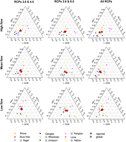
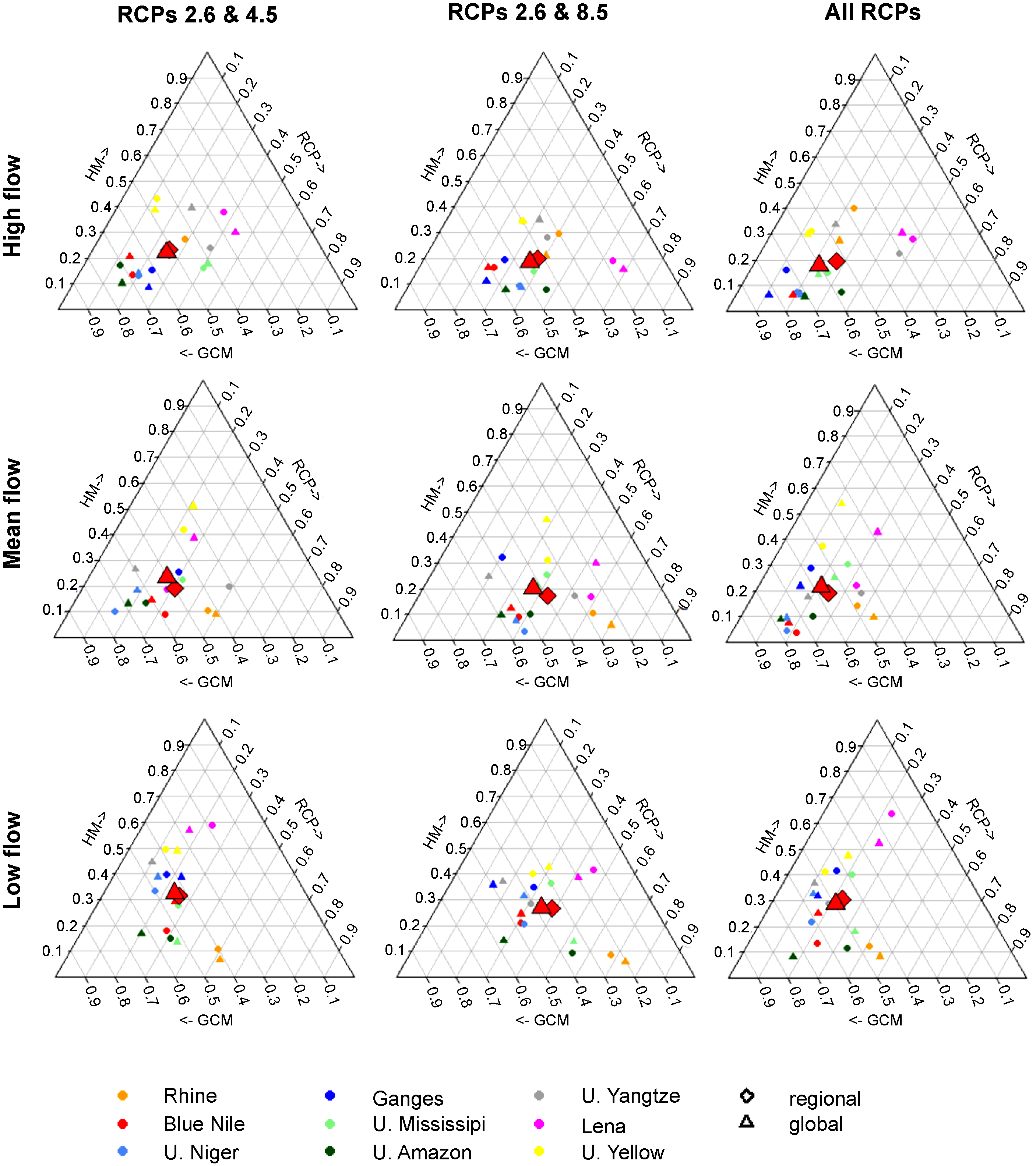
Figure 3. Uncertainty in changes in long-term average river discharge decomposed into its main sources (GCMs, HMs and RCPs) for the high flows (Q10, top), mean flows (Q50, middle) and low flows (Q90, bottom). The left triangle shows the results when considering only RCP2.6 and RCP4.5, the middle one when considering RCP2.6 and RCP8.5 and the right one when considering all RCPs. The smaller symbols indicate individual river basins separately for the global (triangles) and regional hydrological models (diamonds), the bigger icons the mean of the respective group.
Download figure:
Standard image High-resolution image
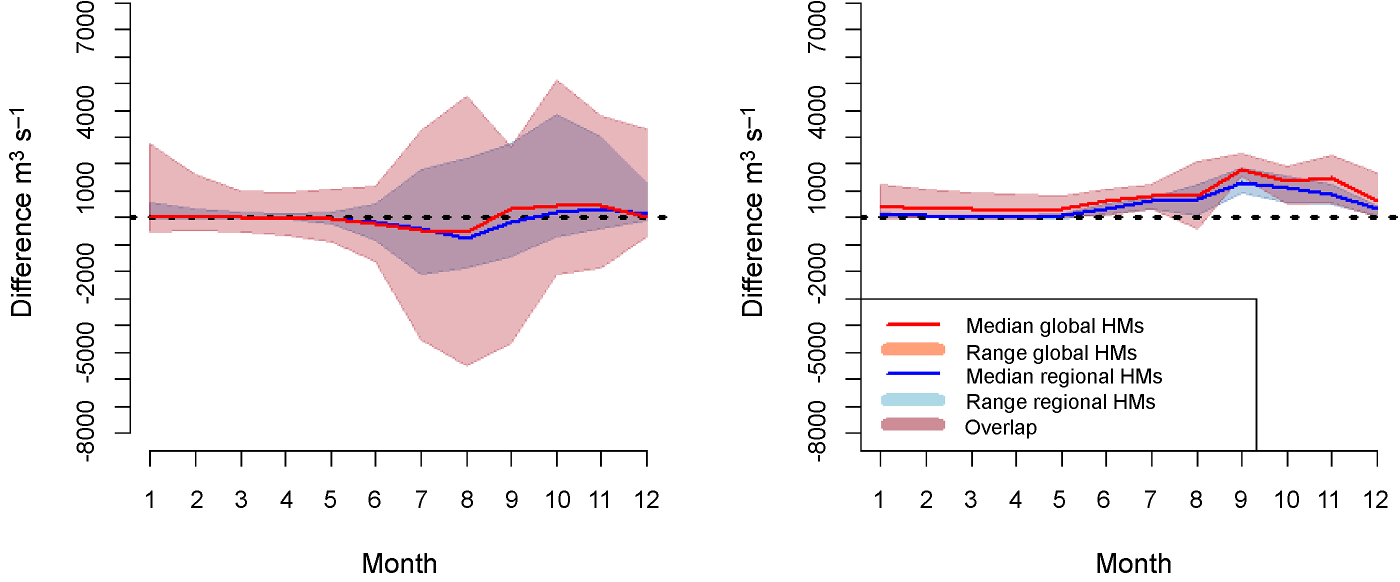
Figure 4. Range of impact uncertainty in the Niger basin (change in discharge at gauge Koulikoro comparing the long-term monthly values of the reference period 1971–2000 and the scenario period 2070–2099) using all GCMs to drive the global and regional HMs (left), and the range of impact uncertainty when the same models are only driven by one GCM (GFDL-ESM2M, right).
Download figure:
Standard image High-resolution image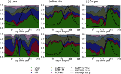
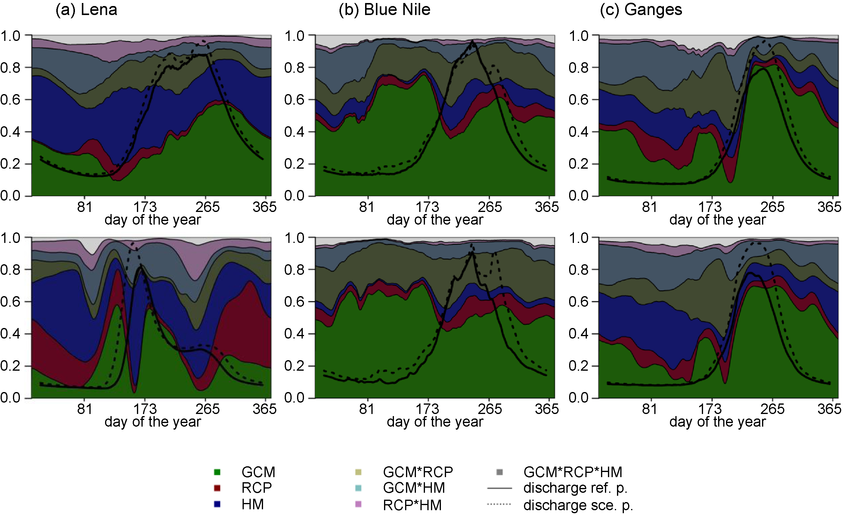
Figure 5. Sources of uncertainty in projected changes in runoff seasonality for the rivers Lena (gauge Stolb), Blue Nile (gauge El Diem) and Ganges (gauge Farakka). The lines give the long-term daily discharge in the reference (1971–2000) and scenario periods (2070–2099). Top: only global HMs considered. Bottom: only regional HMs considered.
Download figure:
Standard image High-resolution imageThere is a tendency that global HMs show higher uncertainty of outputs, but not for the low flows (Q90) in the Ganges and the mean (Q50) and high flows (Q10) in the Blue Nile. More exceptions are the high flow in the Yangtze (both RCPs) and the high flow (Q50) in the Mississippi (figure A1).
The uncertainty in projected river discharge decomposed into its main sources is shown in figure 3. We further distinguish uncertainty decomposition in the ANOVA setting when considering all RCPs (RCP2.6, RCP4.5, RCP6.0 and RCP8.5), when considering only the two moderate scenarios (RCP2.6 and RCP4.5) having only a small difference in global temperature increase, and when considering only the two extreme ones (low end RCP2.6 and high end RCP8.5). The latter one has the strongest difference in global temperature increase (for the individual values see tables A1a–c in the appendix).
Most values are located in the lower left corner when considering only differences in the moderate scenarios RCP2.6 and RCP4.5, but also when accounting for all four RCPs. This indicates the high share of GCM driven uncertainty to the entire uncertainty in river discharge when looking at small differences in temperature increase, where GCM driven uncertainty dominates over the other sources. However, low flows in general and especially in the Lena basin are more sensitive to variation in HMs, because low flows are dominated by hydrological processes such as evapotranspiration, groundwater discharge and in the case of the Lena also by snow thawing processes, which are in different ways implemented in the HMs. The lowest sensitivity to variations in HMs is visible in the Rhine basin, the mean and high flows in the Niger and the high flows in the Ganges and Amazon (figure 3 and tables A1a–c in the appendix). The middle column in figure 3 illustrates that only when looking at larger differences in temperature increases, considering solely the low- and high-end scenarios RCP2.6 and RCP8.5, the scenario (RCP) selection has a larger contribution to the entire uncertainty. It is in most cases higher than the HM related one and the highest in the Rhine basin for the low and mean flows and in the Lena for the high flows. The dominant role of GCMs is also illustrated in figure 4, where the impact uncertainty in the Niger basin is compared when only one GCM (GFDL-ESM2M) is used to drive the HMs and when the scenario results of all five GCMs are applied to drive the impact models: using output of only one GCM gives a clear trend to more discharge, while using output of all five GCMs results in a highly unclear trend with increases and decreases in discharge.
Figure A2 shows that only for low flows and small differences in global temperature increase, HMs contribute a higher share than RCPs. It is also interesting that global and regional HMs show a very similar behavior, despite the differences in impact uncertainty (figure 2), where the variation from global models was higher in most cases.
A deeper insight into seasonal pattern of uncertainty contribution is given in figure 5 considering all four RCPs in the ANOVA setting (for the Lena, Blue Nile and Ganges; for the rest of the basins see figure A3). The uncertainty in the changes in discharge, decomposed into main sources and for the long-term mean values, displays that the uncertainty contributed by the HMs can be considerable in times when the hydrological processes largely determine river discharge. This is the case during the dry season (months November to June in the Ganges) or when snow and soil freezing processes are important. The latter is the case for the Lena River, almost all over the year, but there is particularly high HM uncertainty for the spring flood because the HMs control the magnitude of the snowpack and the rate of melting (Gelfan et al 2017). In dry periods, evapotranspiration and groundwater processes dominate the river discharge pattern, and the different hydrological models use different formulations to reproduce them (see also Hagemann et al 2013). Also notable is the high share of the interaction terms to the total uncertainty in part of the seasonal results. It is the highest when GCMs are involved (GCM⁎RCP and GCM⁎HM in figures 5 and A3) and when, for example, GCM precipitation results are sensitive to scenario conditions (RCPs), but precipitation shows divers trends in different GCM simulations from RCP2.6 to RCP8.5 (positive and negative).
The number of river basins, in which variations in the GCM, RCP and HM settings have a significant effect on river discharge (p-value of the F-test < 0.01), relative to the total number, is given in table 2. The table further distinguishes such cases where the variation in specific boundary conditions is significant within the regional hydrological model ensemble (first number in parenthesis) and when it is significant within the global model ensemble. The fixed ANOVA model is used, meaning that the results of the statistical evaluation apply only to the specific model setting. Notable is that differences in GCM input have always a significant impact on all flow components. The second highest significance has variation in HMs, while the scenario setting (RCPs) has the smallest effect on overall variance in the hydrological impact assessment. When quantifying the influence of small differences in scenario settings (e.g. only small global temperature increase as in RCP2.6 and RCP4.5), this variation results only in two third of the basins in a significant impact on mean discharge. Basins without a significant effect of small temperature differences on mean river discharge are the monsoon driven Upper Niger, Upper Nile and Upper Amazon. Significance modeled by regional and global hydrological models shows no systematic difference.
5. Discussion and conclusions
Our results show that small increases in global temperature can have a statistically significant impact on river discharge for all flow components in almost all basins (table 2), but this effect is often obscured by GCM related uncertainty (figures 3 and 4). This is mostly due to the uncertainty in projected precipitation trends (figure 1). The contribution of GCM related uncertainty is highest in periods of the year, and in regions, where precipitation dominates the river flow regime (figure 5), such as in monsoon dominated basins like the Ganges and Blue Nile. HM related uncertainty is higher in periods of the year, and regions, where snow melt, soil freezing processes and evapotranspiration have a substantial influence on the river regime, for example in the sub-arctic climate of the Lena, mountainous basins or during the dry season in the Ganges and the Blue Nile. The latter is in line with the results of Samaniego et al (2017), who found that droughts will increase in magnitude and duration in most basins they investigated, with a higher share of HM uncertainty but still lower than GCM uncertainty. In addition, Pechlivanidis et al (2017) reported that GCM as well as HM related uncertainty is larger in dry regions. Hagemann et al (2013) pointed out the important role of evapotranspiration in HM related impact uncertainty using a global model ensemble.
Table 2. Results of the significance analysis (F-test). The first value gives the ratio of cases (relative to the total number), where a variation in the respective boundary condition (GCMs, RCPs, HMs) has a significant effect (p-value of the F-test < 0.01) on a flow component of river discharge in the nine river basins. In brackets are the number of cases with significant effect on river discharge in the nine basins modeled by regional hydrological models (first number in brackets) and by global hydrological models (second number in brackets). The fixed ANOVA model is used.
| RCP2.6 and 4.5 | |||
|---|---|---|---|
| Flow component | GCM | RCP | HM |
| low flow (Q90) | 100% (9,9) | 77.8% (6,8) | 100% (9,9) |
| mean flow (Q50) | 100% (9,9) | 66.7% (6,6) | 94.4% (9,8) |
| high flow (Q10) | 100% (9,9) | 72.2% (6,7) | 88.9% (7,9) |
| RCP2.6 and 8.5 | |||
| Flow component | GCM | RCP | HM |
| low flow (Q90) | 100% (9,9) | 83.3% (7,8) | 88.9% (8,8) |
| mean flow (Q50) | 100% (9,9) | 83.3% (8,7) | 88.9% (9,7) |
| high flow (Q10) | 100% (9,9) | 88.9% (7,9) | 88.9% (8,8) |
The dominating influence of GCM-driven uncertainty relative to the total uncertainty is also reported by e.g. Eisner et al (2017), Vetter et al (2017), and Buda et al (2017), all using regional hydrological models in their impact assessments, but using other methodologies or without a rigorous quantification of the statistical significance of the results. Hirabayashi et al (2013) showed, using a global hydrological model, that the uncertainty in global flood risk under climate change is mainly related to the spread of climate models. Results of nine global HMs are analyzed by Dankers et al (2014), who found that HM related uncertainty can predominate over GCM related uncertainty especially in areas with snow melt, while outside the tropics GCM related uncertainty is often not much larger than the HM related one.
We do not see any larger differences in HM related uncertainty in terms of relative changes in discharge when it is simulated by regional or global HMs (figure 3), and the same holds for the significance of variations in HMs (table 2). This supports the results reported in earlier cross-scale investigations. Hattermann et al (2017), for example, found that sensitivity of global and regional HMs to climate variability is comparable in most basins under study, but the analysis of differences in means, medians and spreads revealed many differences between the two HM ensembles and only in two cases of 11 results agreed in all three criteria. Gosling et al (2017) showed that the ensemble median values of changes in runoff with three different magnitudes of global warming (1, 2 and 3 °C above pre-industrial levels) are generally similar between the two ensembles (global and regional HMs), although the ensemble spread is often larger for the global HM ensemble. However, from the sample of HMs included in this study, some differences between the regional and global scale applications can be seen. Most prominently, global HMs in many cases tend to have a stronger increase in impact uncertainty with time than regional HMs (figure 2).
A limitation of our study is that we used only data of five GCMs to drive the HMs. Their simulation results have been compared against the output of the larger GCM ensemble, and in most cases constitute a representative subset (see also Krysanova and Hattermann 2017). Another limitation is that we did not consider model parameter related uncertainty, which can be considerable (Eckhardt et al 2003), but should in most cases not change the direction of the trend.
Summarizing, the results of our study agree with the outcome of previous publications mostly done using scenarios with high temperature increase. Moreover, we show that small increases in global temperature, such as those underlined in the Paris Agreement, have statistically significant impacts on hydrology. However, as GCM uncertainty is so large, a robust trend in water resources and extremes is often only visible when more extreme climate scenarios (and global temperature rises) are considered. The uncertain but nevertheless significant impacts on river discharge (high, low and average flow) demand for intelligent strategies to adapt water use and management in an uncertain future.
The high GCM-related uncertainty is a serious issue and further research is necessary to better understand whether (a) this is due to missing or too simplified processes in climate models, e.g. connected to precipitation processes (clouds, convective events etc), (b) the climate system is in part so complex and uncertainty bounds will remain large, or (c) a rigorous model selection process based on a list of agreed performance criteria should precede any impact study.
Acknowledgments
This work has been conducted under the framework of ISIMIP, funded by the German Federal Ministry of Education and Research (BMBF) with project funding reference number 01LS1201A. Responsibility for the content of this publication lies with the authors. We acknowledge the World Climate Research Programme's Working Group on Coupled Modeling, which is responsible for CMIP, and we thank the respective climate modelling groups for producing and making available their model output. We also acknowledge the support of the Global Runoff Data Centre and of the Environment Research and Technology Development Fund (S-10) of the Ministry of the Environment, Japan. LB would like thank the DFG for funding this work (BR 2238/5-2). The publication of this article was partially funded by the Open Access Fund of the Leibniz Association.
Appendix
Below we show exemplarily the equations to calculate one main effect (equation A1), one first order (equation A2) and one second order interaction term (equation A3):
While Yijk is the specific value corresponding to the climate model i, hydrological model j and RCP k (equation (1)), respectively,  gives the value when averaging over the indexes j and k (HMs and RCPs), and the same way
  when averaging over the indexes i and k (GCMs and RCPs).

Figure A1. Variability in changes in Q50 (mean flow), Q90 (low flow) and Q10 (high flow) based on all simulation results for the RCPs 2.6 and 8.5, separately for the regional and global models (blue and orange curves) for the Mississippi, Amazon, Upper Niger, Upper Yangtze, Upper Yellow and Lena in the period 2030−2100.
Download figure:
Standard image High-resolution image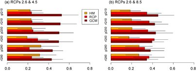
Figure A2. Uncertainty in river discharge decomposed into its main sources (GCMs, HMs and RCPs) for the mean flows (Q50), high flows (Q10) and low flows (Q90) (g–global, r–regional). (a) The results when considering only RCP2.6 and RCP4.5 and (b) when considering RCP2.6 and RCP8.5. The error bars give the standard deviation.
Download figure:
Standard image High-resolution image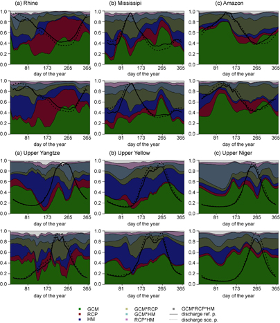
Figure A3. Sources of uncertainty in projected changes in runoff seasonality for the Rhine, Mississippi, Amazon, Upper Yangtze, Upper Yellow and Upper Niger. The lines give the long-term daily discharge in the reference (1971–2000) and scenario periods (2070–2099). Top: only global HMs considered. Bottom: only regional HMs considered.
Download figure:
Standard image High-resolution image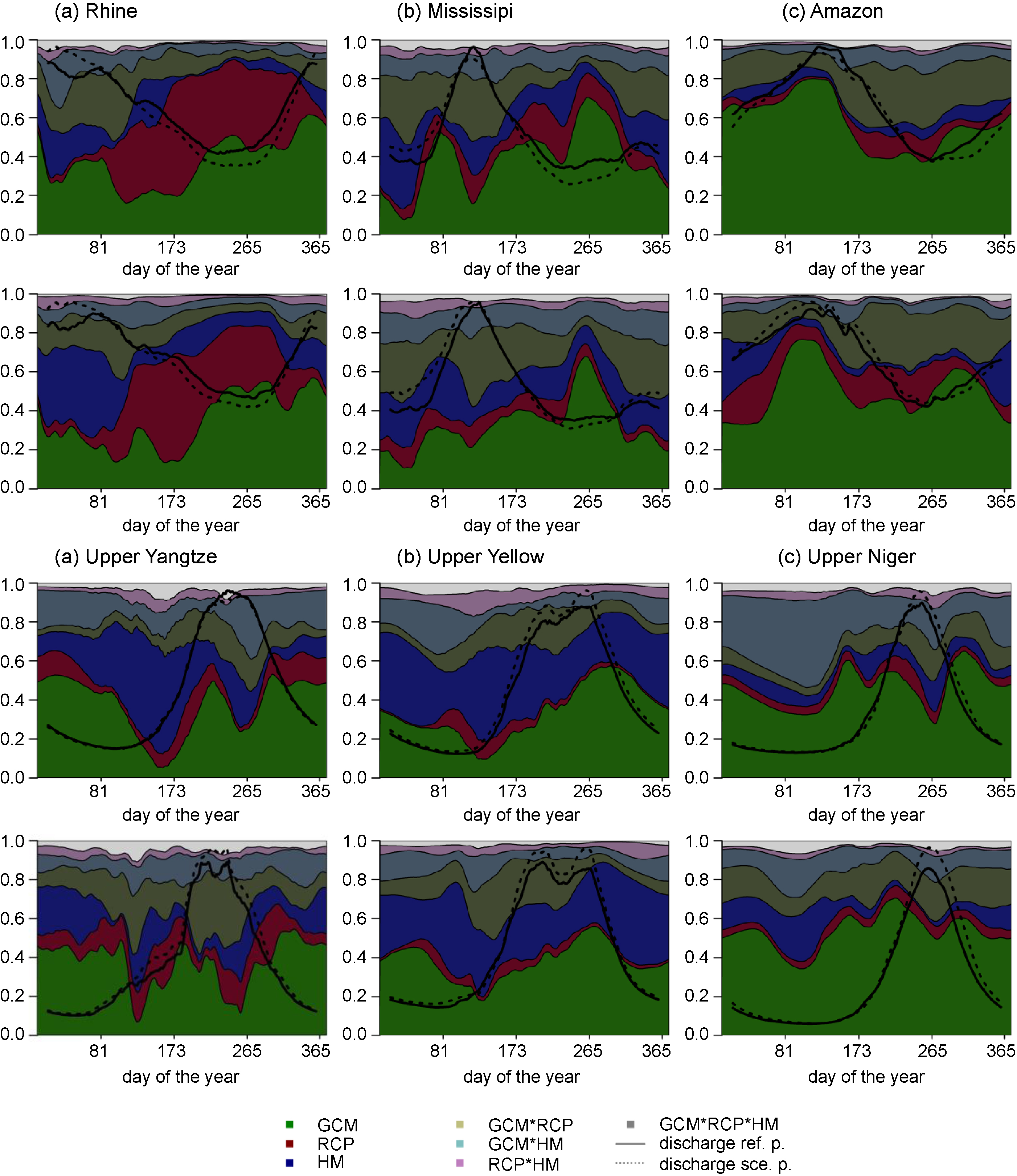
Table A1a. The individual values shown in figure 3 (considering RCPs 2.6 and 4.5).
| Global HM | Regional HM | ||||||
|---|---|---|---|---|---|---|---|
| River | Flow | GCM | RCP | HM | GCM | RCP | HM |
| Rhine | Q90 | 0.4 | 0.49 | 0.11 | 0.41 | 0.51 | 0.07 |
| Blue Nile | Q90 | 0.54 | 0.26 | 0.18 | 0.45 | 0.19 | 0.29 |
| Niger | Q90 | 0.5 | 0.14 | 0.33 | 0.46 | 0.13 | 0.39 |
| Ganges | Q90 | 0.43 | 0.14 | 0.4 | 0.38 | 0.2 | 0.39 |
| Mississippi | Q90 | 0.45 | 0.26 | 0.28 | 0.52 | 0.32 | 0.14 |
| Amazon | Q90 | 0.54 | 0.3 | 0.15 | 0.63 | 0.2 | 0.17 |
| Yangtze | Q90 | 0.44 | 0.22 | 0.29 | 0.45 | 0.08 | 0.44 |
| Lena | Q90 | 0.18 | 0.22 | 0.59 | 0.27 | 0.16 | 0.57 |
| Yellow | Q90 | 0.38 | 0.11 | 0.5 | 0.35 | 0.15 | 0.49 |
| Rhine | Q50 | 0.43 | 0.46 | 0.11 | 0.41 | 0.49 | 0.09 |
| Blue Nile | Q50 | 0.58 | 0.31 | 0.09 | 0.6 | 0.23 | 0.15 |
| Niger | Q50 | 0.75 | 0.14 | 0.1 | 0.63 | 0.18 | 0.18 |
| Ganges | Q50 | 0.45 | 0.28 | 0.26 | 0.49 | 0.3 | 0.19 |
| Mississippi | Q50 | 0.46 | 0.3 | 0.23 | 0.49 | 0.28 | 0.22 |
| Amazon | Q50 | 0.63 | 0.23 | 0.14 | 0.69 | 0.18 | 0.13 |
| Yangtze | Q50 | 0.31 | 0.45 | 0.2 | 0.6 | 0.12 | 0.26 |
| Lena | Q50 | 0.53 | 0.28 | 0.19 | 0.34 | 0.27 | 0.39 |
| Yellow | Q50 | 0.36 | 0.2 | 0.42 | 0.28 | 0.21 | 0.51 |
| Rhine | Q10 | 0.44 | 0.28 | 0.27 | 0.52 | 0.26 | 0.21 |
| Blue Nile | Q10 | 0.69 | 0.17 | 0.13 | 0.66 | 0.13 | 0.2 |
| Niger | Q10 | 0.67 | 0.18 | 0.13 | 0.66 | 0.18 | 0.14 |
| Ganges | Q10 | 0.61 | 0.24 | 0.15 | 0.65 | 0.25 | 0.09 |
| Mississippi | Q10 | 0.43 | 0.39 | 0.16 | 0.41 | 0.4 | 0.18 |
| Amazon | Q10 | 0.71 | 0.1 | 0.17 | 0.74 | 0.12 | 0.1 |
| Yangtze | Q10 | 0.37 | 0.36 | 0.24 | 0.36 | 0.22 | 0.39 |
| Lena | Q10 | 0.26 | 0.35 | 0.38 | 0.26 | 0.43 | 0.3 |
| Yellow | Q10 | 0.45 | 0.11 | 0.43 | 0.48 | 0.12 | 0.39 |
Table A1b. The individual values shown in figure 3 (considering RCPs 2.6 and 8.5).
| Global HM | Regional HM | ||||||
|---|---|---|---|---|---|---|---|
| River | Flow | GCM | RCP | HM | GCM | RCP | HM |
| Rhine | Q90 | 0.24 | 0.67 | 0.09 | 0.2 | 0.73 | 0.06 |
| Blue Nile | Q90 | 0.48 | 0.27 | 0.21 | 0.46 | 0.24 | 0.24 |
| Niger | Q90 | 0.47 | 0.29 | 0.21 | 0.42 | 0.23 | 0.31 |
| Ganges | Q90 | 0.37 | 0.25 | 0.35 | 0.5 | 0.12 | 0.36 |
| Mississippi | Q90 | 0.3 | 0.31 | 0.36 | 0.34 | 0.5 | 0.14 |
| Amazon | Q90 | 0.36 | 0.53 | 0.09 | 0.57 | 0.27 | 0.14 |
| Yangtze | Q90 | 0.41 | 0.28 | 0.28 | 0.46 | 0.16 | 0.37 |
| Lena | Q90 | 0.13 | 0.44 | 0.42 | 0.2 | 0.41 | 0.38 |
| Yellow | Q90 | 0.34 | 0.24 | 0.4 | 0.28 | 0.27 | 0.43 |
| Rhine | Q50 | 0.28 | 0.61 | 0.1 | 0.24 | 0.7 | 0.06 |
| Blue Nile | Q50 | 0.53 | 0.36 | 0.09 | 0.54 | 0.31 | 0.12 |
| Niger | Q50 | 0.54 | 0.41 | 0.04 | 0.55 | 0.37 | 0.08 |
| Ganges | Q50 | 0.47 | 0.18 | 0.32 | 0.56 | 0.17 | 0.25 |
| Mississippi | Q50 | 0.36 | 0.37 | 0.25 | 0.41 | 0.35 | 0.21 |
| Amazon | Q50 | 0.49 | 0.4 | 0.1 | 0.59 | 0.31 | 0.1 |
| Yangtze | Q50 | 0.31 | 0.51 | 0.17 | 0.56 | 0.18 | 0.25 |
| Lena | Q50 | 0.25 | 0.57 | 0.17 | 0.17 | 0.53 | 0.3 |
| Yellow | Q50 | 0.33 | 0.35 | 0.31 | 0.25 | 0.27 | 0.47 |
| Rhine | Q10 | 0.3 | 0.39 | 0.3 | 0.39 | 0.39 | 0.21 |
| Blue Nile | Q10 | 0.58 | 0.23 | 0.17 | 0.61 | 0.21 | 0.16 |
| Niger | Q10 | 0.54 | 0.35 | 0.09 | 0.53 | 0.35 | 0.09 |
| Ganges | Q10 | 0.54 | 0.26 | 0.19 | 0.64 | 0.25 | 0.11 |
| Mississippi | Q10 | 0.46 | 0.38 | 0.15 | 0.44 | 0.36 | 0.17 |
| Amazon | Q10 | 0.45 | 0.46 | 0.08 | 0.59 | 0.32 | 0.08 |
| Yangtze | Q10 | 0.35 | 0.36 | 0.28 | 0.34 | 0.3 | 0.35 |
| Lena | Q10 | 0.17 | 0.62 | 0.19 | 0.15 | 0.68 | 0.16 |
| Yellow | Q10 | 0.4 | 0.25 | 0.35 | 0.4 | 0.25 | 0.34 |
Table A1c. The individual values shown in figure 3 (considering all RCPs).
| Global HM | Regional HM | ||||||
|---|---|---|---|---|---|---|---|
| River | Flow | GCM | RCP | HM | GCM | RCP | HM |
| Rhine | Q90 | 0.47 | 0.4 | 0.12 | 0.45 | 0.46 | 0.08 |
| Blue Nile | Q90 | 0.64 | 0.17 | 0.14 | 0.57 | 0.09 | 0.25 |
| Niger | Q90 | 0.61 | 0.11 | 0.22 | 0.55 | 0.08 | 0.33 |
| Ganges | Q90 | 0.43 | 0.12 | 0.42 | 0.54 | 0.1 | 0.32 |
| Mississippi | Q90 | 0.39 | 0.18 | 0.4 | 0.49 | 0.29 | 0.18 |
| Amazon | Q90 | 0.54 | 0.32 | 0.12 | 0.74 | 0.16 | 0.08 |
| Yangtze | Q90 | 0.52 | 0.15 | 0.29 | 0.53 | 0.08 | 0.37 |
| Lena | Q90 | 0.14 | 0.22 | 0.64 | 0.24 | 0.22 | 0.52 |
| Yellow | Q90 | 0.47 | 0.09 | 0.41 | 0.36 | 0.12 | 0.47 |
| Rhine | Q50 | 0.49 | 0.36 | 0.14 | 0.46 | 0.44 | 0.1 |
| Blue Nile | Q50 | 0.74 | 0.19 | 0.04 | 0.75 | 0.15 | 0.07 |
| Niger | Q50 | 0.77 | 0.16 | 0.05 | 0.75 | 0.14 | 0.09 |
| Ganges | Q50 | 0.57 | 0.12 | 0.29 | 0.64 | 0.12 | 0.22 |
| Mississippi | Q50 | 0.44 | 0.22 | 0.3 | 0.51 | 0.21 | 0.25 |
| Amazon | Q50 | 0.66 | 0.23 | 0.1 | 0.77 | 0.13 | 0.09 |
| Yangtze | Q50 | 0.45 | 0.33 | 0.19 | 0.64 | 0.15 | 0.18 |
| Lena | Q50 | 0.45 | 0.31 | 0.22 | 0.28 | 0.28 | 0.43 |
| Yellow | Q50 | 0.49 | 0.12 | 0.38 | 0.34 | 0.11 | 0.54 |
| Rhine | Q10 | 0.37 | 0.21 | 0.4 | 0.48 | 0.22 | 0.27 |
| Blue Nile | Q10 | 0.72 | 0.19 | 0.07 | 0.75 | 0.18 | 0.06 |
| Niger | Q10 | 0.73 | 0.16 | 0.08 | 0.72 | 0.19 | 0.06 |
| Ganges | Q10 | 0.72 | 0.11 | 0.16 | 0.83 | 0.1 | 0.06 |
| Mississippi | Q10 | 0.59 | 0.24 | 0.15 | 0.62 | 0.21 | 0.14 |
| Amazon | Q10 | 0.58 | 0.34 | 0.07 | 0.71 | 0.21 | 0.06 |
| Yangtze | Q10 | 0.31 | 0.41 | 0.23 | 0.47 | 0.17 | 0.34 |
| Lena | Q10 | 0.23 | 0.45 | 0.28 | 0.26 | 0.43 | 0.3 |
| Yellow | Q10 | 0.56 | 0.12 | 0.31 | 0.58 | 0.11 | 0.3 |