

Abstract
Seasonal climate forecasts could be an important planning tool for farmers, government and insurance companies that can lead to better and timely management of seasonal climate risks. However, climate seasonal forecasts are often under-used, because potential users are not well aware of the capabilities and limitations of these products. This study aims at assessing the merits and caveats of a statistical empirical method, the ensemble streamflow prediction system (ESP, an ensemble based on reordering historical data) and an operational dynamical forecast system, the European Centre for Medium-Range Weather Forecasts—System 4 (S4) in predicting summer drought in Europe. Droughts are defined using the Standardized Precipitation Evapotranspiration Index for the month of August integrated over 6 months. Both systems show useful and mostly comparable deterministic skill. We argue that this source of predictability is mostly attributable to the observed initial conditions. S4 shows only higher skill in terms of ability to probabilistically identify drought occurrence. Thus, currently, both approaches provide useful information and ESP represents a computationally fast alternative to dynamical prediction applications for drought prediction.
Export citation and abstract BibTeX RIS

Original content from this work may be used under the terms of the Creative Commons Attribution 3.0 licence.
Any further distribution of this work must maintain attribution to the author(s) and the title of the work, journal citation and DOI.
1. Introduction
Ecosystems and human societies are strongly impacted by weather driven natural hazards, such as droughts [1, 2], expected to become more frequent and of larger amplitude under climate change [3–6]. Seasonal climate forecasts of droughts can enable a more effective adaptation to climate variability and change, offering an under-exploited opportunity to minimise the impacts of adverse climate conditions. Consequently, developing skilful drought seasonal forecasts has become a strategic challenge in national and international climate programs (see e.g. [7]).
The feasibility of seasonal prediction by mean of numerical models largely rests on the existence of slow, and predictable, variations in soil moisture, snow cover, sea-ice, and ocean surface temperature, and how the atmosphere interacts and is affected by these boundary conditions [8]. Seasonal predictability of weather events is spatially as well as seasonally highly variable. Generally, the skill is high over the tropics while over the extra-tropics it is very limited. Over Europe, the achieved forecast skill is low, especially regarding seasonal rainfall forecasts [8, 9]. However, recent investigations have shown some improvements with the initialization of soil moisture [10], increased resolution [11] and some systems have demonstrated skill in prediction of the large scale circulation over Europe up to a year in advance [12].
Meteorological drought predictions, defined using the standardized precipitation index aggregated over several months (such as SPI–6, that is, aggregated over 6 months; [13]), generated with dynamical models combined with monitored data indicate significant skill (see [14] for a global assessment using ECMWF-System 4 data (S4) and [15, 16] using the North-American Multi-Model Ensemble).
Thus, it is essential to compare dynamical climate predictions with simple empirical methods to assess the overall added value of the former [17]. For instance, [14] found that it is difficult for dynamical systems to add value with respect to forecasts based on climatology. Instead, [15] found some added value of dynamical forecasting relative to a baseline empirical method when predicting the drought onsets. They consider as a benchmark forecast an ensemble streamflow prediction (ESP; [18]) system. The ESP method relies on resampled historical data to generate an ensemble of possible future climate outlooks. [19] have achieved skillful predictions of several drought indicators at global scale with this method, showing the value of purely statistical based systems.
Skill of both empirical and dynamical methods largely relies on the persistence properties of droughts. Long observational datasets that are continuously updated are thus of paramount need to monitor current conditions and to generate drought indicator forecasts [20]. However, a number of constraints (such as data unavailability and poor data coverage) may limit such analysis. This is particularly challenging when observations need to be available in near-real time (so less time is available to retrieve and control the observations) and especially over data-poor regions (e.g. Africa and South America [16]).
Previous drought forecast studies (see e.g. [14–16, 19]) are based on the Standardised Precipitation Index (SPI). Recently, many other works have used the Standardized Precipitation Evapotranspiration Index (SPEI) [21]. As the SPI, the SPEI has the advantage of allowing the analysis of different temporal scales. However, the SPEI also includes the effects of temperature on drought assessment [21]. Importantly, summer SPEI has been shown to capture better than other indices (such as SPI or the Palmer drought severity index) the drought impacts on hydrological, agricultural, and ecological variables (e.g. [22–26]).
The aim of this study is to explore the drought seasonal predictability by combining observed climate conditions (with near-real time datasets) with forecasts of the current-summer precipitation and temperature variables based on the ECMWF System-4 and the ESP method. The final goal is to assess the skill achieved by these approaches and drawing some general conclusions about their respective drawbacks and the advantages when applied to the region under investigation. Here we extend previous studies on drought seasonal prediction by (i) analysing the SPEI, (ii) focussing on Europe (between 36.25° to 71.25° N and −16.25° to 41.25° E), a challenging domain for the currently available global dynamical climate models but with good monitoring products (see e.g. [16]) and (iii) evaluating forecasts valid during the boreal summer for the 6-month (relative to the period March to August), when the high heat and associated evaporation are intensifying potential water deficits and shaping drought events with large negative impacts (e.g. on public water supply [27], agriculture [28] and forest fires [29, 30]).
2. Data and methods
2.1. Data
As reference data we used two long term and continuously updated databases: GHCN-CAMS for two-meter air temperature [31] and CPC Merged Analysis of Precipitation (CMAP; [32]). CMAP is a monthly precipitation database from 1979 to near the present and it combines observations and satellite precipitation data into 2.5° × 2.5° global grids. These datasets are consistent with other observational data sets over Europe [31, 32]. Supplementary S1 shows the high consistency between SPEI calculated with these data against SPEI calculated with ECMWF re-analysis data (ERA-Interim) for two-meter temperature [33] and GPCP Version 2.2 Combined Precipitation dataset [34].
Here, we use seasonal forecasts from ECMWF System 4, a leading operational seasonal prediction system based on a fully coupled general circulation model [35]. To evaluate the S4 prediction quality we use a set of retrospective forecasts (re-forecasts) emulating real predictions for a 30-year period (1981–2010) joined with the operational S4 forecast for the period 2011–2015. S4 probabilistic predictions consist in an ensemble of integrations [35] of the model that uses slightly different initial conditions: for the atmosphere the ERA-Interim re-analysis [33] is perturbed using single vector perturbations [36] and for the ocean the 5 members of the ORAS4 reanalysis are used [37].
Temperature and precipitation S4 predictions are bias corrected by means of simple linear scaling performed by using a leave-one-out cross-validation, i.e. excluding the forecasted year when computing the scaling parameters. Figures S2-S9 show the remaining bias (generally negligible), correlation for raw data and for detrended data for monthly temperature and precipitation forecasts from ECMWF System 4 considering the start dates of April, May, June and July. These analyses indicate that the dynamical seasonal forecasts show good performance for the first month, while afterwards their quality declines markedly with remaining correlation skill only locally for temperature at lead time of 2 months or more.
To compare the various data sets, their values are remapped (bilinear interpolation for temperature and conservative remapping for precipitation) from their original resolution to the coarsest grid, defined by CMAP (2.5° × 2.5°). More details on the remapping procedure are provided in the supplementary material available at stacks.iop.org/ERL/12/084006/mmedia.
2.2. Observed SPEI
We calculate the standardized precipitation evapotranspiration index (SPEI) for the 6 month period from March to August. The SPEI considers the monthly climatic balance as precipitation (PRE) minus potential evapotranspiration (PET) and it is obtained through a standardization of the 6-month climatic balance values. The standardization step is based on a nonparametric approach in which the probability distributions (p) of the water balance data samples are empirically estimated [38].
2.3. Predicted SPEI
In this study we assess the skill of forecasts initialized in April, May, June and July for the two prediction systems, S4 and ESP. In both cases, to calculate the predicted SPEI6 for August, we combine the seasonal forecasts of precipitation and temperature with the antecedent series of observed records. For instance, when we forecast SPEI6 with prediction initialized in April (thus performing a 5-month ahead prediction), we aggregate the observed precipitation and temperatures in March with the forecasted values for April to August.
When considering the S4 predictions, we join each individual member prediction of PRE and PET with antecedent observations to obtain an ensemble prediction.
ESP consists in replacing monthly forecasts by resampled historical observations of PRE and PET. Thus, it provides a probabilistic prediction in which each member of the ensemble corresponds to one resampled year, thus preserving the observed sequence in that year. A detailed description of the ESP is provided in [19] and our specific implementation is reported in the supplementary material. All the forecasts are done by using cross-validation in order to evaluate the predictions as if they were done operationally.
2.4. Verification metrics
First, we compute the Pearson correlation coefficient among forecasts and observations on a grid point by grid point basis. We estimate the grid point p-values using a one-sided Student's t test and we correct individual significance tests for multiple hypotheses testing using the False Discovery Rate (FDR) method [39]. We apply the test on the p-values and conservatively set a false rejection rate of q = 0.05. Also, we estimate the significance of the difference between two correlations using the method described in [40], which considers the dependence from sharing the same observations in both correlation values.
Then we compute the reliability diagrams, a common diagnostic of probabilistic forecasts that shows for a specific event (e.g. moderate drought) the correspondance of the predicted probabilities with the observed frequency of occurrence of that event [41]. We also include the weighted linear regression through the points in our diagrams (following [9]).
Also we consider the ROC area skill score (ROCSS) based on the relative operating characteristic (ROC) diagram. ROC shows the hit rate (i.e. the relative number of times a forecast event actually occurred) against the false alarm rate (i.e. the relative number of times an event had been forecast but did not actually happen) for different potential decision thresholds [42].
In order to have a large sample of probability forecast, the reliability diagrams and the ROCSS are computed by aggregating the grid point forecasts within the domain of study following the procedure recommended by the WMO [43]. Thus, for each drought event (e.g. moderate drought, table 1) and grid point, we calculate the forecast probabilities of that event occurring using the ensemble members distribution. Then, we group the probability forecasts into bins (here five of width 0.2) and count the observed occurrences/non-occurrences. Finally we sum these counts for all area-weighted grid points in the studied domain.
We estimate the uncertainties in the reliability slopes and the ROCSS score using bootstrap resampling, where the prediction and observation pairs are drawn randomly with replacement 1000 times. The confidence interval is defined by the 2.5th and the 97.5th percentiles of the ensemble of the 1000 bootstrap replications. To account for the spatial dependence structure of the data, we use the same resampling sequence for all grid points within each bootstrap iteration.
More details on data and methods are provided in the supplementary material.
3. Results
In order to evaluate the deterministic performance of the systems, figure 1 shows the correlation of the S4 predictions (left panels) and the difference between the S4 and the ESP correlations (right panels). Significant S4 correlations exist for all the forecast times, with the highest values for the forecasts initialized in July, as one may expect (figure 1 left panels). Generally S4 and the ESP show similar correlations (figure 1 right panels) with higher scores in the southern and in the eastern sectors of the domain for the S4 predictions initialized in April and May, with few grid points with a p-value <0.05 (not collectively significant considering the FDR test). Looking more in detail, although correlation values give an idea of the overall performance and its evolution with the lead-time, the correlation results for individual grid points should be considered with caution as we are dealing with gridded monthly data, i.e. data showing a strong spatial correlation. This strongly reduces the effective number of independent data and suggest interpreting with care the local results.
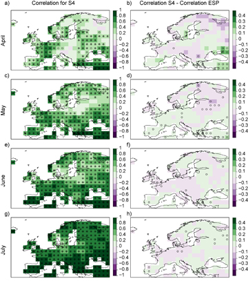
Figure 1 Correlation maps of S4 forecasts of summer SPEI against observed SPEI over the period 1981–2015 (panels (a), (c), (e) and (g), for forecasts are initialized in April, May, June and July, respectively) and difference in correlation between S4 and ESP predictions (panels (b), (d), (f) and (h)). Open circles indicate local significant (i.e. without the FDR correction) correlations (p-values < 0.05); filled points indicate global significant (i.e. after the FDR correction) correlations.
Download figure:
Standard image High-resolution imageIn order to summarize the results and to assess the contribution of the trend to the skill, figure 2 displays the distribution of the correlation values of the pairs (S4 predictions, observations) and (ESP predictions, observations) computed across the studied area for all the different predictions, calculated on both original (figure 2(a)) and linearly detrended data (figure 2(b)). To avoid artificial skill, the data were de-trended in each step of the cross-validation (as recommended by the WMO, [43]).
Three main conclusions can be drawn from this analysis. First, the skill increases with the month of initialisation, as expected. That is, the correlation values in longer leads (i.e. the 5-month ahead prediction issued in April or the 4-month ahead prediction issued in May) are generally lower than those of shorter (2 and 3 months) lead forecast. Second, similar results are obtained considering raw and detrended data, with slightly lower correlation values in the latter case. Third, figure 2 confirms that S4 and ESP perform quite similarly, although usually S4 predictions issued in April and May show slightly better results than ESP ones. Additionally, as expected, the interquartile range of spatial correlation distribution decreases as the starting date approaches July. This indicates that spatial homogeneity of the drought forecast skill is increasing with longer observational precipitation period included in the drought index calculation.
Figures S10 and S11 show the correlation for all the predictions and confirm the above described results. Calculating the Spearman correlation in addition to the Pearson correlation, or quadratic detrending instead of linear detrending, led to similar results (figure S12). It is worth to mention that trends and their significance have been estimated by using the original series, i.e. without applying any pre-whitening procedure. Autocorrelation and trend influence each other and affect the assessment of the associated statistical significance; however, reducing the potential effects of autocorrelation by pre-whitening has in some cases serious drawbacks (see e.g. [44]). To assess the effect of temporal autocorrelation of the data on the significance of our results, we calculate the annual lag-1 autocorrelation coefficients of the observed SPEI series on a grid point by grid point basis and found them to be significant in around 5% of the studied domain (see figure S13). Thus, errors due to serial correlation could be considered negligible. Nevertheless, we also repeat the correlation analysis estimating the significance level of correlation using the Student distribution with N degrees of freedom, N being the effective number of independent data calculated following the method described in [45, 46], obtaining very similar results (figure S14).
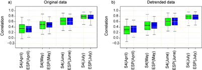
Figure 2 Boxplots of the distribution of the correlation values of the pairs (S4 predictions, Observations) and (ESP predictions, Observations) computed across the studied area for different start dates based on (a) original data and (b) detrended data. The median is shown as a solid line, the boxes indicate the 25–75 percentile range while the whiskers show the 2.5–97.5 percentile range.
Download figure:
Standard image High-resolution imageTable 1. Drought severity classification based on the SPEI values.
| Standardized index | Description |
|---|---|
| −0.50 to −0.79 | Abnormally dry |
| −0.80 to −1.29 | Moderate drought |
| −1.30 to −1.59 | Severe drought |
| −1.60 to −1.99 | Extreme drought |
| −2.0 or less | Exceptional drought |
Figure 3(a) shows the reliability diagram for the studied domain for moderate drought events (SPEI < − 0.8; see table 1 and [47]). It compares the observed relative frequency against the predicted probability, providing a quick visual assessment of the reliability of the probabilistic forecasts. A perfectly reliable system should draw a line as closely as possible to the diagonal (slope equal to 1). Both prediction systems (ESP and S4 initialized in April) show that the uncertainty range of the reliability line does not include the perfect reliability line, however they are inside the skilful BSS area (Brier Skill Score > 0 and slope > 0), that is, they are still very useful for decision-making [9]. In order to summarise the results for all the start dates and drought thresholds, we calculate the slopes (and associated uncertainties) of both predictions (see boxplots of figure 3). Generally the S4 slopes are positives but less than the diagonal, indicating that the forecasts have reliability although tend to be underconfident (a systematic error). On the other hand, generally the ESP slopes are larger than S4 slopes resulting in higher reliability except for the highest drought threshold (although results for the highest drought threshold should be treated with caution since the reduced data sample sizes). Most probable reasons for these results are: (i) ESP resamples the observations (equally well for the whole sample distribution), which allows it to have an adequate spread by definition as it does not have systematic errors associated with the ensemble generation as dynamical models have and (ii) for more extreme events, ESP cannot simulate those cases because they have not been recorded in observational data.
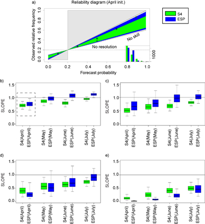
Figure 3 (a) Reliability diagrams for moderate drought predictions (as defined in table 1) for S4 and ESP systems (start date of April). The shaded lines show a linear weighted regression with its 2.5–97.5% confidence level in agreement with [9]. The number of samples for each bin is shown in the lower right sharpness diagram; (b) boxplots of the reliability measured as the slope of the regression line of the reliability diagrams as a function of the start date of the predictions. The median is shown as a solid line, the boxes indicate the 25–75 percentile range while the whiskers show the 2.5–97.5 percentile range. The black horizontal line shows the perfect reliability line (slope = 1). Square with dashed lines indicate the example of figure 3(a). (c), (d) and (e) as (b) but for the severe, extreme and exceptional drought thresholds (according to table 1), respectively.
Download figure:
Standard image High-resolution imageThe reliability diagram measures the performance of the predictions conditioned on the forecasts (i.e. considering the relative number of times an event was observed when it had been forecasted). Complementary information is given by the ROC diagram, which is conditioned on the observations. Figure 4(a) shows an example of the ROC diagram for the prediction initialized in April. It indicates that both the systems have high skill since their curves are both above the identity line H = F (when a forecast is indistinguishable from a completely random prediction). Figures 4(b), (c), (d) and (e) summarize the ROCSS for all the drought thresholds and start dates. At a first glance, it is clear that the skill improves as a function of the start date, although it is worth noting that all the forecasts have some level of skill (ROCSS > 0), except for the ESP prediction issued in April for more severe droughts (figures 4(d) and (e)). Of the predictions, generally S4 shows higher skill compared to that one of the ESP forecasts, especially for the start dates of April and May and for the most severe drought events.
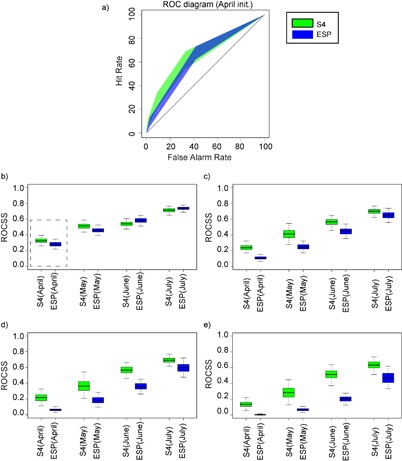
Figure 4 (a) ROC diagrams for moderate drought predictions for S4 and ESP systems (start date of April). The shaded regions indicate the 2.5 and 97.5 confidence intervals calculated through 1000 bootstrap replications. The hit rate and false alarm rate values are considering a set of probability forecasts by stepping a decision threshold with 20% probability through the forecasts. (b) boxplot distribution of the ROCSS values of all the prediction in the south-west region. The median is shown as a solid line, the boxes indicate the 25–75 percentile range while the whiskers show the 2.5–97.5 percentile range. Square with dashed lines indicate the example of figure 4(a). (c), (d) and (e) as (b) but for the severe, extreme and exceptional drought thresholds (according to table 1), respectively.
Download figure:
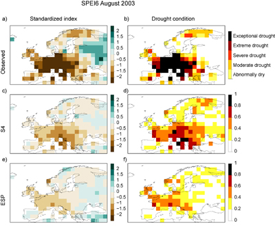
Standard image High-resolution imageThe skill estimates based on the performance of the system in the past may guide end-users on the expected performance of the future forecasts. As an illustrative application, we compare the ability of the drought prediction based on climatological values (ESP) with the dynamical forecasts merged to observations (S4) in forecasting the 2003 drought. This event has been shown to be predictable four months ahead [48, 49]). The observed SPEI (figures 5(a) and (b)) indicates that most of Europe experienced drought conditions, with central Europe reaching SPEI value less than −2, i.e. exceptional drought conditions. Figures 5(c) and (d) show the SPEI6 forecasted for August 2003 using the S4 forecasts initialized in May. Both predictions correctly indicate negative SPEI values over extended regions in Europe, although with milder drought conditions with respect to the observed ones. In addition to the ensemble-mean forecast, we also show the probability for moderate drought occurrence (SPEI < − 0.8). Indeed, having an ensemble of predictions (one SPEI6 prediction for each ensemble member of the S4 system) enables us to provide the probability of drought occurrence for any given drought threshold. This 4-month lead time forecast captures reasonably well the observed drought conditions. Also the ESP prediction issued in May (figures 5(e) and (f)) shows a relatively high agreement with the observations, although both the ensemble mean and the probabilities seem to underestimate the observed ones, more than the S4 predictions.
4. Conclusions and discussion
In this study we have explored the summer drought predictability in Europe through the SPEI indicator aggregated over the months March–August. We have compared two different seasonal forecasting systems: (i) a dynamical prediction system based on the ECMWF System-4 and (ii) the ensemble streamflow prediction system ESP based on reordering historical data. Both systems merge observations with forecasts. Results show that both systems are skilful already a few months ahead suggesting a window of opportunity.
Figure 5 Observed 6-month SPEI for August 2003: (a) SPEI6 values and (b) observed drought conditions (based on table 1). Predicted SPEI6 for August 2003 with the start date of May: (c) S4 ensemble mean; (d) S4 probability for moderate drought occurrence (SPEI < 0.8); (e) ESP ensemble mean and (f) ESP probability for moderate drought occurrence.
Download figure:
Standard image High-resolution image
Moreover, the two systems achieve comparable skill in predicting drought at seasonal time scales. Since the ESP predictability comes from the observed initial drought conditions, we conclude that predictability found here largely relies on the persistence of drought events. We also confirm the main results of previous studies [14, 15, 50] indicating the need of improved dynamical forecasts in the mid-latitude regions in order to add value with respect to a baseline empirical method. Only locally in southern/western Europe and for April and May initializations, we found generally slightly higher performance of S4 in term of correlation values. Some level of reliability of probabilistic forecasts is also shown while the ROC diagram shows generally higher S4 skill compared to the ESP in discriminating drought events.This may be explained by the overall good performance of dynamical seasonal forecasts for the first month of prediction and residual skill afterwards for temperature over this area. Thus, at the moment, ESP represents a computationally faster and cheaper alternative to dynamical prediction applications for drought, and it could be used to benchmark other models.
Nevertheless, our results demonstrate the feasibility of the development of an operational early warning system in Europe. Due to inherent and large uncertainties in seasonal forecasts (both empirically or dynamically based), predictions need to be expressed probabilistically. Our probabilistic verification results suggest that operational forecasts of summer drought in Europe can be attempted, but users need to be well trained on how to best interpret and use these forecasts, given the not-optimal reliability here shown. For instance, from the users perspective, it is important to assess whether these forecasts can predict the occurrence of drought events and it is important to know if the predicted probabilities correspond to the observed probability of the events. A calibration of probability forecasts might be necessary in the opposite case to make the forecasts reliable (e.g. by using the variance inflation technique as applied in [51]). Although these kind of predictions (S4 or ESP) are fine when there is an already established drought, additional studies are needed to forecast the onset and the end of these events [15], for which other systems, based on shorter accumulation scales, have been already evaluated [52].
This work has provided the first assessment of meteorological drought seasonal prediction in Europe, and can also serve as a baseline study for future analyses including other dynamical forecast systems, more sophisticated empirical methods [53], more complex estimation of the PET [54, 55], other hydrological variables (e.g. [56, 57]), and higher resolution.
The results described here are obtained by following a solid, relatively simple and transparent statistical methodology that can also be applied to other areas. In order to ease the reproducibility of the methods and results, and to facilitate the applicability of these predictions, all the scripts used for this study and the SPEI data (observed and predicted) are freely available for research purposes by contacting the corresponding author. In this context, it is worth noting that the ability to generalize the methods themselves is technically straightforward, but the development of a prototype of an operational forecast system is feasible only where/when reliable observed climate variables are available in near-real time. Indeed, a large obstacle to apply these methods in other areas may be in the uncertainties of the observed near-real time data used for drought monitoring and to develop and evaluate the predictions [16, 58]. Thus, it is recommended that, before implementing our approach in other regions, a careful assessment of the available data sets (update in near-real time) should be performed.
Acknowledgments
We acknowledge the NOAA/OAR/ESRL PSD, Boulder, Colorado, USA, for making the data available on their website http://www.esrl.noaa.gov/psd/. This work was partially funded by the Projects IMPREX (EU–H2020 PE024400) and SPECS (FP7-ENV-2012-308378). Marco Turco was supported by the Spanish Juan de la Cierva Programme (IJCI-2015-26953).