

Abstract
Globally emitted contaminants accumulate in the Arctic and are stored in the frozen environments of the cryosphere. Climate change influences the release of these contaminants through elevated melt rates, resulting in increased contamination locally. Our understanding of how biological processes interact with contamination in the Arctic is limited. Through shotgun metagenomic data and binned genomes from metagenomes we show that microbial communities, sampled from multiple surface ice locations on the Greenland ice sheet, have the potential for resistance to and degradation of contaminants. The microbial potential to degrade anthropogenic contaminants, such as toxic and persistent polychlorinated biphenyls, was found to be spatially variable and not limited to regions close to human activities. Binned genomes showed close resemblance to microorganisms isolated from contaminated habitats. These results indicate that, from a microbiological perspective, the Greenland ice sheet cannot be seen as a pristine environment.
Export citation and abstract BibTeX RIS

Original content from this work may be used under the terms of the Creative Commons Attribution 3.0 licence.
Any further distribution of this work must maintain attribution to the author(s) and the title of the work, journal citation and DOI.
Introduction
Greenland ecosystems are influenced by anthropogenic contaminants [1], mostly brought by long-range atmospheric transport [2]. Industrial emissions have resulted in the deposition of contaminants on the Greenland ice sheet (GrIS) since the 1850s [3]. Heavy metals mercury and lead, and persistent toxic compounds such as dichloro-diphenyl-trichloroethan (DDT) and polychlorinated biphenyls (PCB) are well-known contaminants in Greenland and have been found to bio-accumulate in the food chain [1]. Polycyclic aromatic hydrocarbons (PAHs) have been found on the GrIS [4]. As contaminants become trapped within the snow and ice of the cryosphere, these habitats can be considered as reservoirs of toxic chemicals [2].
Climate warming and the resulting increased melting of the cryosphere is causing increased release of contaminants in the polar regions [2, 5]. Melting glaciers are becoming secondary sources of contaminants, including persistent organic pollutants (POPs) such as polychlorinated biphenyls (PCBs) [2, 6]. Dynamic interconnections exist between historic and current emissions for POPs, the cryosphere and climate change, as manifested by the increased release of POPs from Alpine glaciers since the 1990s [5].
The knowledge of the role of microbial communities in the fate of Arctic contamination has been identified as a knowledge-gap [2]. Cultured isolates from cryoconite (glacier surface debris) communities are known to be able to degrade xenobiotics including PCBs [7]. Cryoconite microbial communities from the GrIS incubated under in situ conditions have been shown to degrade pesticides [8] and recently metabolomic data has indicated in situ catabolism of 2,4-dichlorophenoxyacetic acid by cryoconite microbiota from the GrIS [9]. Microbial communities sampled from cryoconite holes (glacier surface melt features containing mineral-microbe aggregates) have also been shown to harbor genes associated with heavy metal resistance [10]. It has been suggested that bacteria in snow might lower the risk of bio-available mercury being incorporated into Arctic food chains [11]. The potential for mercury reduction among microbes in Arctic coastal waters has been found to be able to account for most of the Hg(0) that is produced in high Arctic waters [12]. In the culturable fraction of Bacteria in snow from the high Arctic, 31% of the community were shown to be mercury-resistant, compared to less than 2% in proximate environments of freshwater and brine [11]. Mercury concentrations in snow have been found to correlate with mercury resistance gene copy numbers of snow microbiota [13]. These results suggest that cryospheric microbial communities interact with anthropogenic contaminants and might be able to remove a fraction of the contaminants deposited to this environment before they are released to downstream ecosystems [8].
In this study we demonstrate the potential for resistance to and degradation of anthropogenic contamination by microbial communities sampled from cryoconite around the GrIS. We assessed the genetic potential to resist and utilize contaminants including PCBs, polycyclic aromatic hydrocarbons (PAHs), and heavy metals mercury and lead via shotgun metagenomic sequencing and binning of bacterial genomes. To the best of our knowledge this is the largest shotgun metagenomic dataset of cryoconite to date, and the first investigation that puts focus on the Greenland ice sheet surface as a contaminated habitat.
Materials and methods
Sampling
Sampling has been described previously [14, 15]. In short, 34 cryoconite samples were collected from the GrIS in five different locations between May and September 2013. Sampling sites included Tasiilaq (TAS) in Southeast Greenland, Qassimiut (QAS) in Southwest Greenland, Kangerlussuaq (KAN) in West Greenland, Dark Site (DS) in West Greenland, inland from the Disko Bay area, and Thule (THU) in Northwest Greenland (figure 1).
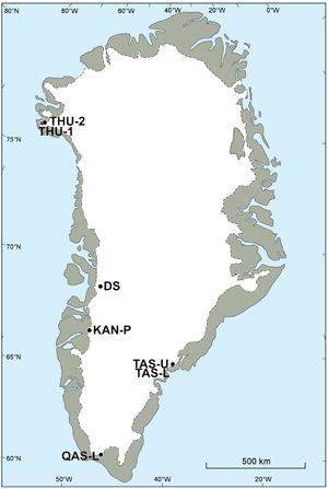
Figure 1 Map of sampling sites. TAS = Tasiilaq, THU = Thule, DS = Dark Site (one of the darkest 5 km pixels in optical satellite imagery [15]), KAN = Kangerlussuaq, QAS = Qassimiut. Sample details have been described previously [14,15].
Download figure:
Standard image High-resolution imageLibrary preparation and sequencing
DNA extraction was performed as described previously [14]. DNA shearing and library preparations were performed according to the
NEXTflex Rapid DNA-Seq Kit, V13.08 (Bioo Scientific, Austin, TX, USA).
Briefly, 250 ng genomic DNA was sheared by Covaris E210 System using 10% duty cycle, intensity of 5 cycles per burst of 200 for 300 seconds to create 200 bp fragments. The samples were end-repaired and adenylated to produce an A-overhang. Adapters containing unique barcodes were ligated on to the DNA. Samples were then purified using bead size selection to select for 300–400 bp fragments using the Agercount AMPure XP beads (Beckman Culter, Beverly, MA, USA).
The purified DNA libraries were amplified with a denaturation time of 2 min at 98 °C, followed by 12 cycles of denaturation at 98 °C for 30 seconds, annealing at 65 °C for 30 seconds and extension at 72 °C for 1 minute according to the protocol. The final extension was performed at 72 °C for 4 min. DNA quantification was performed using a NanoDrop ND-1000 UV-VIS Spectrophotometer (Thermo Fisher Scientific, Waltham, MA, USA) and the quality was checked on an agilent 2100 Bioanalyzer using the Bioanalyser DNA High sensitivity kit (Agilent Technologies, Santa Clara, CA, USA). Library preparation was performed by in-house facilities (DTU Multi-Assay Core (DMAC), Technical University of Denmark). DNA libraries were mixed into 9 pools in equimolar ratios, resulting in 5 samples per sequencing lane. Sequencing was performed as a 100 bp paired-end run on a HiSeq 2000 (Illumina Int., San Diego, CA, USA) following the manufacturer's recommendations. The metagenomic data is available on the NCBI Sequence Read Archive through accession number PRJNA360211.
Demultiplexing and data quality check
The number of different barcodes in raw sequencing files was counted prior to demultiplexing into individual sample files. This was done in order to confirm that all barcodes were represented in roughly equal numbers in the sequencing output, and to check for contamination. Demultiplexed files for each of the samples from nine lanes of Illumina HiSeq sequencing were concatenated to obtain one complete sample file in fastq format [16]. Data quality was assessed using FastQC version 0.11.2 [17] and reads were trimmed for bad quality bases and Illumina adaptors using Cutadapt [18] through MGmapper version 2.5 [19]. Cutadapt settings were used with a minimum phred score for base quality of 30, and minimum read length of 30 bp.
Scaffold assembly and gene calling
Quality trimmed fastq files were assembled using idba_ud assembler version 1.1.1. with pre-correction [20]. Prokaryotic open reading frames were called using Prodigal version 2.6.2 [21].
Binning of genomes
Files with genes called by Prodigal for each sample were concatenated into a gene catalogue and each entry was given a unique header. The gene catalogue was clustered to reduce homology at 95% identity using USEARCH package cluster_fast version 8.1.1861 [22]. Centroids from the clustering were used in downstream analyses. For each sample, raw reads were mapped against the indexed gene catalogue using bwa mem version 0.7.12 [23]. Samtools version 0.1.18 [24] was used to sort and convert sam format files from mapping to bam format files. An in house python script was used to count the number of reads mapping to genes in the gene catalogue. Read counts were assembled into a count matrix with a perl script (Script 1 supplementary material). The count matrix was rarefied to the depth of the shallowest sample with a depth of 49 671 209 read counts per sample. This was done using the Vegan package rrarefy [25] in R Studio version 0.99.903 [26]. Genome bins were clustered based on gene co-abundance with the Canopy Clustering method with a maximum canopy distance of 0.1 and a maximum merge distance of 0.05 [27]. A total of 29 bins with correlation to profile > 0.95 and between 3000 and 8000 genes were assembled from contigs to which binned genes belonged. The quality of the binned genomes was tested with Checkm [28]. The genomes were annotated and further assessed in RAST [29]. Putative genomes are accessible through RAST guest user, username 'guest' and password 'guest', genome IDs are listed in supplementary table 2 available at stacks.iop.org/ERL/12/074019/mmedia. When comparing binned genomes with control genomes in RAST the control genomes used were Escherichia coli 536 publicly available in RAST (control 1), Lactobacillus casei ATCC 334 also publicly available in RAST (control 2) as well as Belliella baltica DSM 15883 [30] (control 3).
Taxonomic composition
MGmapper version 2.5 [31] was used to remove PhiX and map reads from each sample against genome databases of Bacteria and Bacteria draft genomes. Results from mapping to the bacterial databases were used for making stacked barplot of taxonomic composition. Quality filters for mapped reads to be included in taxonomic composition were; properly paired reads with alignment scores of >30, minimum coverage of 80% resulting in minimum identity of 86% and a minimum of 10 reads to be mapped to a strain for it to be evaluated as true.
Differential potential for degradation of xenobiotics and heavy metal resistance
Genes in the rarefied count matrix were annotated by blasting against the KEGG database [32] using Diamond blastx version 0.7.9 [33], resulting in BLAST tabular m8 format sequence IDs. Only genes from the original gene catalogue with blast hits E-value < 1e-50 were included in counts. There were several genes in the count matrix with identical sequence IDs although the count matrix is based on homology-reduced genes. This can be explained by the fact that homology reduction is sequence based and entries in the count matrix from different parts of a gene would have the same annotation but would not be combined in the homology reduction step (USEARCH cluster_fast). The counts of identical sequence IDs were combined (Script 2 supplementary material) and information on gene names and EC-numbers were added to each entry in the annotated and combined count matrix (Script 3 supplementary material). Entries in the count matrix with identical gene names and EC-numbers were combined (Script 4 supplementary material).
The contaminants for which the genetic potential for degradation or resistance was assessed were selected based on known contaminants in the Arctic food chain [1].
Based on KEGG [32] K0 numbers or gene names the number of reads mapping to responsible genes was extracted from the rarefied count matrix.
For PCB degradation K08689, K08690, K00462 and K10222 were found in the count matrix [32]. For PAH degradation EC-numbers 1.1.1.256, 1.13.11.3, 1.13.11.38, 1.13.11.8, 1.14.12.12, 1.14.12.15, 1.14.12.7, 1.14.13.1, 1.14.13.23, 1.2.1.78, 1.3.1.19, 1.3.1.29, 1.3.1.49, 1.3.1.53, 1.3.1.64, 3.1.1.35, 4.1.1.55, 4.1.1.69, 4.1.2.34 were searched for [32]. For heavy metal resistance genes czc, chr, ncc and mer [34] as well as Pbr [35] genes were extracted from the count matrix.
Of the other contaminants listed as important for the Arctic food chain [1] PFOS were not assessed as evidence suggests that these are not degraded by bacteria [36]. PBDEs were also not assessed as it is still unknown which genes are responsible for degradation [37].
For plotting the number of reads mapped to degradation and resistance genes and for comparison between samples, the total number of reads mapped to target genes were divided by the total number of reads mapped to the 14 genes that have been found to be present in most bacterial genomes [38]. This was used as a measure of an internal constant, since the number of these genes could be expected not to differ between organisms. In this way, we obtained an approximation of the fraction of degradation and resistance genes per sample.
Two metagenomic samples of healthy human gut were run through the same pipeline as described above. These samples were used as negative controls, and in particular, to confirm that genes detected for contaminant degradation and resistance were not background artifacts. Human gut metagenomes were downloaded from the European Nucleotide Archive study PRJEB1220 [27]. We assumed that the healthy human guts were non-contaminated. None of the contaminant related genes were found in the negative controls.
Results and discussion
Metagenomic samples were binned into 29 genomes through de novo clustering by co-abundance genes (supplementary figure 1). Of the 29 genome bins, 24 were successfully annotated in RAST (table 1), and 13 bins were complete genomes based on the content of their marker genes (table 1; supplementary figure 1). The strain heterogeneity of detected marker genes was above 90% for 11 of the 13 bins that were 100% complete (table 1). GC content ranged between 35.4% and 66.2% (mean = 57.7 ± 9.8).
Table 1. Genome bin overview. Closest neighbors are automatically assigned in RAST with the use of a neighbor score. The neighbor score is the number of times that the 'neighbor' genome is the top BLAST hit against a candidate gene from the set of 'unique' genes within the query genome. The closest neighbor does not necessarily indicate the taxonomy of the query genome but indicates similarity in assigned functions between the query genome and the closest neighbor.
| Bin ID | Complete-ness | Contamina-tion | Strain heterogeneity | Size (bp) | GC content (%) | Closest neighbor in RAST (score) | Phylum | Family |
|---|---|---|---|---|---|---|---|---|
| 81 | 100 | 548,45 | 99,52 | 23062772 | 64.5 | Acidiphilium cryptum JF-5 (501) | Proteobacteria | Acetobacteraceae |
| 59 | 100 | 384,08 | 95,25 | 15614510 | 58.8 | Acidobacterium sp. MP5ACTX9 (516) | Acidobacteria | Acidobacteriaceae |
| 58 | 100 | 910,4 | 99,08 | 34698014 | 66 | Frankia sp. EuI1c (532) | Actinobacteria | Frankiaceae |
| 51 | 100 | 116,65 | 79,66 | 8649830 | 44.5 | Chitinophaga pinensis DSM 2588 (581) | Bacteriodetes | Chitinophagaceae |
| 50 | 100 | 707,64 | 97,73 | 26578570 | 35.4 | Chitinophaga pinensis DSM 2588 (542) | Bacteriodetes | Chitinophagaceae |
| 47 | 100 | 1305,01 | 95,36 | 38823998 | 65.4 | Caulobacter sp. K31 (513) | Proteobacteria | Caulobacteraceae |
| 45 | 100 | 571,82 | 91,33 | 26076195 | 58.7 | Acidiphilium cryptum JF-5 (525) | Proteobacteria | Acetobacteraceae |
| 41 | 100 | 782,94 | 98,52 | 33343276 | 57.9 | Acidobacterium sp. MP5ACTX9 (511) | Acidobacteria | Acidobacteriaceae |
| 35 | 100 | 1051,64 | 99,63 | 38873183 | 65.2 | Chloroflexus aggregans DSM 9485 (393) | Chloroflexi | Chloroflexaceae |
| 34 | 100 | 728,28 | 97,53 | 31824964 | 36.8 | Chitinophaga pinensis DSM 2588 (613) | Bacteriodetes | Chitinophagaceae |
| 28 | 100 | 767,26 | 52,11 | 27944005 | 64.8 | Clavibacter michiganensis subsp. michiganensis NCPPB 382 (526) | Actinobacteria | Microbacteriaceae |
| 22 | 100 | 651,67 | 98,87 | 37385964 | 49.2 | Nostoc sp. PCC 7120 (648) | Cyanobacteria | Nostocaceae |
| 21 | 100 | 1117,12 | 94,33 | 48259586 | 63.3 | Streptosporangium roseum DSM 43021 (503) | Actinobacteria | Streptosporangiaceae |
| 77 | 98,28 | 300,52 | 80,03 | 9563229 | 63.4 | Mucilaginibacter paludis DSM 18603 (838) | Bacteriodetes | Sphingobacteriacea |
| 18 | 98,09 | 376,32 | 93,83 | 23602306 | 56.8 | Ktedonobacter racemifer DSM 44963 (549) | Chloroflexi | Ktedonobacteraceae |
| 63 | 96,55 | 164,54 | 90,64 | 9599541 | 64.7 | Acidiphilium cryptum JF-5 (522) | Proteobacteria | Acetobacteraceae |
| 73 | 95,83 | 463,02 | 98,19 | 18407868 | 66.2 | Acidiphilium cryptum JF-5 (514) | Proteobacteria | Acetobacteraceae |
| 48 | 95,83 | 348,87 | 98,45 | 17680617 | 65.4 | Gluconacetobacter diazotrophicus PAl 5 (522) | Proteobacteria | Acetobacteraceae |
| 29 | 95,83 | 668,8 | 99,58 | 26933316 | 63.3 | Solibacter usitatus Ellin6076 (501) | Acidobacteria | Solibacteraceae |
| 09 | 95,83 | 432,39 | 64,45 | 36290647 | 62.4 | Leptothrix cholodnii SP-6 (507) | Proteobacteria | Unclassified |
| 84 | 95,61 | 107,35 | 80,77 | 5422601 | 60.7 | marine actinobacterium PHSC20C1 (537) | Actinobacteria | Unclassified |
| 30 | 92,11 | 75,41 | 93,02 | 10047939 | 47.3 | Desulfuromonas acetoxidans (501) | Proteobacteria | Desulforomonadaceae |
| 40 | 88,95 | 95,22 | 6,67 | 8729345 | 40.7 | Pedobacter heparinus DSM 2366 (583) | Bacteriodetes | Sphingobacteriacea |
| 69 | 67,46 | 43,03 | 9,09 | 3811046 | 62.9 | Leifsonia xyli subsp. xyli str. CTCB07 (517) | Actinobacteria | Microbacteriaceae |
The closest neighbors of resulting putative genomes were one Cyanobacterium (Nostoc sp. PCC 7120), five Proteobacteria, five Actinobacteria, three Bacteroidetes, two Acidobacteria and two Chloroflexi (table 1). The taxonomy of the closest neighbor is not necessarily the taxonomy of the query genome but rather an indication that the genomes share functions. The phyla of the closest neighbors were among the most abundant (>1%) in the metagenomic samples (figure 2). Half of the genome bins belong to families shown to represent >1% of OTUs in the sampled sites according to a previous study based on 16S rRNA gene amplicon sequencing [14]. These were Acetobacteraceae, Acidobacteriaceae, Solibacteraceae, Microbacteriaceae, Chitinophagaceae, Sphingobacteriaceae, and Nostocaceae (table 1). 16S SSU rRNA genes were located in the binned genomes and nucleotide sequences were blasted against the NCBI nr/nt database. Top matches are listed in supplementary table 2. Due to either incompleteness or contamination of the binned genomes as shown in table 1 and supplementary figure 1 some genomes had 0 or several 16S SSU rRNA genes, which may not be from the same actual genomes. Additionally, the extracted 16S SSU rRNA genes are not full length and span different regions of the gene, which adds some uncertainty compared to targeted amplicon sequencing of 16S SSU rRNA genes. Therefore the taxonomic indications of the putative genomes should be regarded with caution.
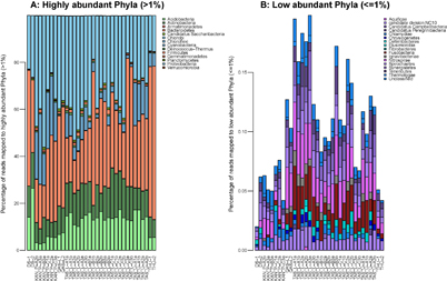
Figure 2 Taxonomic composition across samples of (a) most abundant Phyla (>1%) and (b) low abundant Phyla (≤1%).
Download figure:
Standard image High-resolution imageMean richness, calculated as CatchAll alpha diversity of samples grouped by area, was previously estimated to be between 31 and 116 species per group based on 16S rRNA gene sequencing [14]. The 18 species found among the binned genomes potentially made up between 15.5% and 58% of the community.
Organisms isolated from contaminated habitats or known to be resistant to contaminants were among the closest neighbors to the binned genomes. The closest neighbor of bin 9, Leptothrix cholodnii SP-6, has received interest as a potential bioremediation organism due to its ability to oxidize iron and manganese, and its potential ability to sequester heavy metals [39]. Frankia sp. strain EuI1c, the closest neighbor of bin 58, belongs to a group of organisms known to be less sensitive to heavy metals such as lead and arsenic [40]. This strain in particular has been shown to have cellular mechanisms for increased copper tolerance [41]. The closest neighbor of bin 47, Caulobacter sp. K31, was isolated from chlorophenol-contaminated groundwater and has the ability to tolerate copper and chlorophenols [42]. Four of the bin genomes (bins 81, 45, 73 and 63) were closest neighbors to Acidiphilium cryptum JF-5, which was isolated from acidic coal mine lake in eastern Germany and was shown to be able to reduce Fe(III) [43]. These binned putative genomes indicate that cryoconite holes on the GrIS contain organisms with the ability to survive and utilize the presence of long-distance transported contaminants.
The percentages of genes in pathways (RAST active subsystems) related to resistance to and degradation of contaminants were compared among the genome bins listed above, and with the genomes of known organisms that are not from cryoconite, namely Escherichia coli, Lactobaccillus casei, and Belliella baltica, an isolate from the Baltic Sea [30], as controls.
There were a number of active subsystems associated with contaminants, for which some binned genomes had a comparably high percentage of genes (figure 3). Bin 9 (nearest neighbor Leptothrix cholodnii SP-6) had a notably high percentage of genes for zinc resistance (figure 3(a)). Bin 73 (nearest neighbor Acidiphilium cryptum JF-5) had high percentages of genes in mercuric reductase, copper tolerance, and resistance to chromium compounds as well as metabolism of aromatic compounds (figure 3(b)–(e)). In general, the binned genomes had higher percentages of genes in metabolism of aromatic compounds when compared to the controls (figure 3(e)).
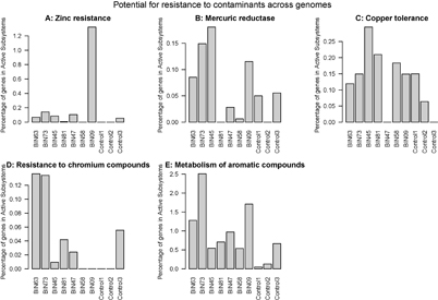
Figure 3 Percentage of genes in contamination-associated active subsystems of the total number of genes in active subsystems within each genome (count data from RAST). Control genomes were organisms known from other habitats: Escherichia coli 536 (control 1), Lactobacillus casei ATCC (control 2) as well as Belliella baltica DSM 15883 (control 3).
Download figure:
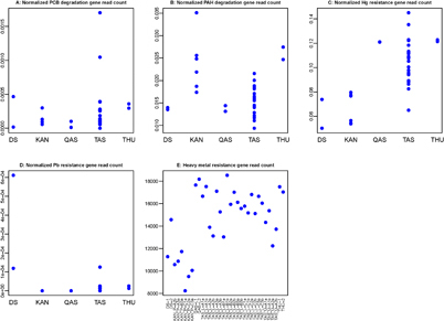
Standard image High-resolution imageSamples from all the sites had reads that mapped to PCB degradation genes (figure 4(a)). Counts of reads mapped to PCB degradation genes were variable between samples taken from each region. The highest number of reads that mapped to PCB degradation genes were found among the TAS samples from Tasiilaq in Southeast Greenland, ranging from 0 (TAS-U-A1b) to 145 (TAS-L-C3b) reads per sample (normalized counts 2.8 × 10⁻⁴ ± 3.8 × 10⁻⁴) (figure 4(a), supplementary table 1). Two TAS samples had more than twice as high counts of PCB degradation genes compared to all of the other samples (1.70 × 10⁻³ and 1.05 × 10⁻³ PCB degradation reads/housekeeping reads).
Figure 4 Read counts normalized to counts of reads mapped to housekeeping genes for reads mapped to (a) PCB degradation genes, (b) PAH degradation genes (c) Mercury resistance genes, (d) Lead resistance genes and (e) general heavy metal resistance genes. Note that counts in panel E have not been normalized to housekeeping genes.
Download figure:
Standard image High-resolution image
For PAH degradation genes, the KAN samples from Kangerlussuaq had the most reads mapped to these genes followed by the THU (Thule) samples (figure 4(b)). The relatively high abundance of PAH degradation genes in the KAN samples contrasts the observations from the other contaminant degradation genes, which were found to be in relatively low abundances at KAN (figures 4(a), (c)–(e)). PAHs are generated primarily through the incomplete combustion of organic materials such as oil, petrol and wood [44]. The PAH content in snow from the Kangerlussuaq region was assessed previously under the hypothesis that the proximity of the site to the largest airport of Greenland would result in a PAH contamination [4]. While PAH contamination was found to be below detection limit in the study, the results were inconsistent with previous results and well below the concentrations found in near-by cryosphere environments [4, 45, 46]. The relatively high abundance of reads mapping to PAH degradation genes in Kangerlussuaq and Thule samples might be explained by the proximity of both of these sites to large aviation centers (Kangerlussuaq International Airport, and Thule Air Base respectively).
The number of reads that mapped to mercury resistance genes ranged from 4644 (KAN-P-A2b) to 10283 (TAS-L-B1b) (unnormalized counts 7671 ± 1586.5). The highest normalized read count of mercury resistance genes was found in the TAS samples (figure 4(c)). The two QAS and the two THU samples had similar counts, which were intermediate between the high TAS samples and the lower counts in the DS and KAN samples (figure 4(c), supplementary table 1). Mercury concentrations have been measured in the KAN, QAS, TAS and THU regions [4]. Concentrations were lower in snow from Kangerlussuaq (KAN) and higher in the South (QAS) and Southeast (TAS) (supplementary figure 2(a)), which parallels with read count data (figure 4(c)). Inuit from Tasiilaq in Southeast Greenland have also been shown to have higher contamination with PCBs and mercury in recent years [1]. In contrast, reads for DDT degradation were not found in any of the samples.
Lead resistance read counts were found to have very high numbers in one of the DS samples in West Greenland and no reads in KAN and QAS samples in Southwest and South, respectively. The number of reads that mapped to lead resistance genes ranged between 0 to 71 (unnormalized counts 3.18 ± 12.32). The DS-1 sample had almost six times as many reads mapped to lead resistance genes as the other samples (figure 4(d)). In general, the KAN samples had lower numbers of reads mapped to the combined set of heavy metal resistance genes (figure 4(e)). Lead concentrations on the GrIS have been measured to be slightly higher in the Thule (THU) region (supplementary figure 2(b)) [4]. Read counts of lead resistance genes (figure 4(d)) do not seem to follow previously measured lead concentrations (supplementary figure 2(b)).
Inuit lead contamination has been shown to be similar across Greenland with slightly lower contamination in Tasiilaq in Southeast Greenland [1], in contrast to other contaminants (figures 4(a)–(c), (e)), and in resemblance to the observations for reads mapped to lead resistance genes in cryoconite (figure 4(d)).
Further research is needed to clarify whether GrIS supraglacial microbial communities may serve as indicators for first entry of contaminants into the Arctic food chain, which would have implications for the release of contaminants into the food chain as a result of climate warming. This notion is not unlikely knowing that the copy number of resistance genes correlates with contaminant concentrations in snow [13], and melting of the cryosphere has been shown to release contaminants into the downstream ecosystems [2, 5, 6].
Our results show that microbial communities on the GrIS have the potential for resistance to and degradation of contaminants known to be transported to the Arctic.
The potential for resistance and degradation was found to be spatially variable, yet present at all sites around the GrIS and not limited to single sample sites or samples in close proximity to human activity. While the potential was present at all sites this study is geographically limited to the GrIS. Decreasing costs of metagenomic analyses and the expected increase in the availability of metagenomic datasets from supraglacial habitats will allow the comparison across the terrestrial cryosphere. Future research might reveal whether there is a broader trend in the degradation of xenobiotics within the terrestrial cryosphere.
As a negative control the same assessment was carried out in two metagenomes from healthy human gut samples. The human gut metagenomes had no reads that could be mapped to any of the genes included in the cryoconite assessment above. These results suggest that the deposition of contaminants onto the GrIS may influence the supraglacial microbial community composition and function. Consequently, the GrIS should not be considered a pristine environment.
Previous work has shown that gene copy numbers of resistance genes correlate with contaminant concentrations in snow [13], which suggests that the presence of contaminant-related genes in microbial communities on the GrIS are a response to the presence of the relevant contaminants. Metabolomic data from the GrIS indicate in situ catabolism of 2,4-dichlorophenoxyacetic acid by cryoconite microbiota [9]. However, no measurements of the contaminants tested in the current study exist from the sampled sites, and it is not clear whether or not the genes are expressed. Results from the binned genomes are based on active subsystems only, which does indicate that the genes are parts of functional systems in the organisms. Further research is needed to establish the link between contaminant deposition on the GrIS and the functional diversity of the present microbes.
Contamination of supraglacial environments is constantly occurring and contaminants from past depositions are locked into the ice at certain depths [47]. Concentrations of bioavailable contaminants in cryoconite holes may be dependent on the historic deposition events of the exposed ice surfaces. In this respect, thousands of years old contamination might become available to current cryosphere communities. It has been established that current contaminations in higher trophic levels are largely caused by past events [48]. This might also hold true for microbial communities, particularly in supraglacial habitats, where contaminants are locked in the ice.
Conclusions
The metagenome of microbial communities in cryoconite collected on the Greenland ice sheet shows the potential for resistance to and degradation of contaminants, including polychlorinated biphenyls (PCB), polycyclic aromatic hydrocarbons (PAHs), and the heavy metals mercury and lead. The presence of genes for contaminant resistance and degradation was spatially variable but present in all samples across the ice sheet. Binned genomes showed close resemblance to the genomes isolated from contaminated habitats. Since the genetic potential of contaminant resistance and degradation usually indicates the presence of the relevant contaminants, the Greenland ice sheet should not be considered a pristine environment, and more attention should be paid to the potential release of anthropogenic contaminants from this fast-changing environment.
Acknowledgments
This work was partly supported by the Novo Nordisk Foundation Center for Biosustainability, the Center for Permafrost (CENPERM) Center no 100 from the Danish National Research Foundation (DNRF100) as well as Dudo and Povl Brandt's Foundation. This work was also supported by a Villum Young Investigator Programme grant VKR 023121 to MS. KC is a Sêr CYMRU II COFUND fellow who is also supported by the Sêr Cymru National Research Network for Low Carbon, Energy and Environment.