

Abstract
Wind power generation in Great Britain has increased markedly in recent years. However due to its intermittency its ability to provide power during periods of high electricity demand has been questioned. Here we characterise the winter relationship between electricity demand and the availability of wind power. Although a wide range of wind power capacity factors is seen for a given demand, the average capacity factor reduces by a third between low and high demand. However, during the highest demand average wind power increases again, due to strengthening easterly winds. The nature of the weather patterns affecting Great Britain are responsible for this relationship. High demand is driven by a range of high pressure weather types, each giving cold conditions, but variable wind power availability. Offshore wind power is sustained at higher levels and offers a more secure supply compared to that onshore. However, during high demand periods in Great Britain neighbouring countries may struggle to provide additional capacity due to concurrent low temperatures and low wind power availability.
Export citation and abstract BibTeX RIS

Original content from this work may be used under the terms of the Creative Commons Attribution 3.0 licence.
Any further distribution of this work must maintain attribution to the author(s) and the title of the work, journal citation and DOI.
Corrections were applied to this article on 4 October 2017. The affiliations for David J Brayshaw were amended.
1. Introduction
The British Government is committed to reducing greenhouse gas emissions whilst maintaining a resilient and affordable energy supply. Britain has an ambitious target to achieve 15% of its energy consumption (electricity, heat and transport) from renewable sources by 2020 [1]. Policy measures have led to an increase in the percentage of energy consumption generated from renewables, from 3% in 2009 to 8% in 2015. Wind power accounted for approximately half of the renewable electricity generated in 2015 and it is therefore already playing an important role in the British energy system [2]. Offshore wind capacity is expected to grow significantly over the next decades [2, 3], in part to help meet the increase in electricity demand expected with the electrification of heating and transportation.
Operational managers ensure electricity supply and demand are balanced second by second. To achieve this, forecasts of demand and supply are made in the months, days and hours prior to real time. Peak demand is a primary concern, and the grid operator must ensure ahead of each winter that sufficient supply is available. This is of growing importance due to an increased security of supply risk in Britain in recent years, associated with closing of older coal and gas plants [4, 5]. The intermittent nature of wind power means that estimating its availability in advance is challenging. A better knowledge of the relationship between electricity demand and wind power supply is therefore advantageous, especially during peak demand. The availability of interconnection supply from neighbouring countries during peak British demand is also of growing interest, due to increasing interconnector capacity and the participation of interconnectors in the Capacity Market (a system developed to ensure security of supply) [6].
The influence of weather on the demand–supply balance is increasing, due to the high temperature sensitivity of demand [7, 8] and increasing renewable generation. Consequently, interest in this issue is growing [9–15]. A weak positive relationship is found between electricity demand and wind power supply across the year in Britain [9], with the reverse found in winter [13, 15]. However during very high demand conditions, some studies suggest the risk of lower wind power supply [10, 13, 15], whilst others suggest more moderate or higher supply [9, 11, 16]. They all emphasize the uncertainty in the relationship due to the short data lengths considered (often less than 10 years). Large scale weather patterns have been shown to influence electricity demand and renewable supply over Northern Europe, including the North Atlantic Oscillation [12, 14] (NAO, a measure of the large scale north–south atmospheric pressure difference), and high pressure systems. The influence of high pressure on wind power supply and demand is however under debate [10, 16, 17].
The aim of the paper is to quantify the winter relationship between daily electricity demand and wind power supply across Great Britain (GB) over an extended period (34 years). The role of weather patterns on this relationship is explored, with a particular focus on high demand conditions. The wider European context is then considered, by assessing temperature and wind power conditions across Europe during periods of high GB demand.
2. Data and methodology
2.1. Electricity demand data
An observed electricity demand dataset was provided by National Grid, the grid operator, for the period January 1975 to March 2013. This dataset gives the total electricity demand across GB for each day in giga watt hours (GWh). Annual electricity demand is shown to steadily increase from 1975 until 2006 and then reduce [8]. The magnitude of the annual cycle in demand is also found to reduce over the whole period. These long term changes in demand cannot be explained by temperature changes, rather are thought to be predominantly driven by socio-economic factors [8].
To better quantify the relationship between weather driven electricity demand and wind power, these long term changes in demand are firstly removed. This is achieved by representing the evolution of the annual mean demand and annual cycle by a slowly evolving second order Fourier expansion. This slowly evolving background is then removed from the full demand time-series and is replaced by a repeating long term mean annual demand cycle [8]. This process effectively retains the demand variability on a daily, seasonal and interannual timescale, whilst removing variability on timescales greater than 5 years. Full details of the detrending methodology are given in sections 3 and 4 of Thornton et al [8], where the original and detrended electricity demand time-series are shown (figure 1 and supplementary figure 7 respectively).
2.2. Wind power model
Wind power availability is modelled using reanalysis wind speeds and an idealised wind power model. In the latter, a uniform distribution of turbines across GB is assumed, including both onshore and coastal offshore regions (see figure 7 in supplementary material available at stacks.iop.org/ERL/12/064017/mmedia). Regions under consideration for siting of future offshore turbines have also been included, for example in the North Sea. The uniform distribution approach does not attempt to accurately represent current-day generation, but rather it aims to capture the general variation in available wind power across GB and through time. This approach has the additional benefit of giving information on possible future generation sites.
A daily wind power estimate is calculated using 6-hourly, 60 m height wind speeds and air density from the ERA-Interim dataset. ERA-Interim is a gridded global reanalysis dataset, with a resolution of approximately 80 km by 80 km and is available from January 1979 to the present. A reanalysis dataset is created by rerunning a global weather model over a long period, whilst ingesting all available observations. It provides a multivariate, spatially complete and coherent record of atmospheric circulation [18].
The wind speed at each ERA-Interim grid-point is fed through a typical power curve, the Vestas V90 1.8–2 MW turbine6 is chosen with a cut in, cut out and rated wind speed (Ur) of 4 m s−1, 25 m s−1 and 12 m s−1 respectively. A wind power capacity factor is then calculated as follows:

where U represents the wind speed after it has been modified by the power curve characteristics, ρ is the air density and ρc = 1.225 kg m−3, a typical density. The capacity factor therefore takes both wind speed and air density changes into account.
The wind power capacity factor is calculated at each grid point, every 6 hours and then averaged to give a daily mean, for all days between 1979 and 2013. In addition a regional mean capacity factor is calculated for each day, from the daily mean values. The resultant wind power capacity factors should be considered as indicative, rather than numerically exact, given the idealised wind power model used. Even with these simplifications, the modelled GB average capacity factor in winter (∼0.5) is found to compare favourably with a study where the wind farm distribution and capacity are more realistically represented [15]. Given the idealised wind power model used, we consider the electricity demand and wind power separately, rather than combining to give a proportion of demand met by wind power.
3. Electricity demand, wind power relationship
The electricity demand–wind power relationship is calculated over the period for which both datasets are available (January 1979 to March 2013). The relationship is only calculated over week days (Monday–Friday) during non–holiday periods. Weekends, bank holidays and 3 days either side of bank holidays are excluded from the analysis due to the different demand profiles seen over these non-working days [8]. The data considered therefore represents 62% of the full data set and consists of 7804 days.
To put the winter relationship between electricity demand and wind power in context, we start by showing the relationship across the year and in each season. A clear seasonal cycle in demand is seen, with lowest demand in summer and highest demand in winter (figure 1, upper left). A wide range of wind power conditions exist for a given electricity demand, and the range is smallest in summer and largest in winter.

Figure 1 Upper left: Scatter plot of daily GB electricity demand and GB mean wind power capacity factor in winter (blue), spring (green), summer (orange) and autumn (brown). Density contour interval is 0.02%. Pink lines show the median demand and capacity factor across all days. Upper middle: Variation in GB average wind power capacity factor with percentile of electricity demand, averaged over a 5% demand bin, for each season (colours) and all days in year (black). A minimum of 18 values (1% of that seasons' days) are required to make a mean capacity factor. Upper right: For a given level of demand, the percentage of days in each season. Lower: Scatter plot of winter daily electricity demand and wind power when averaged across GB (left), offshore region (middle) and onshore region (right).
Download figure:
Standard image High-resolution imageDuring the lower three-quarters of demand days, there is the seemingly helpful relationship that as demand increases so does average wind power [9] (black line figure 1, upper middle). This reflects the variation in temperatures and wind speeds with season, with calmer, warmer conditions in summer and cooler, windier conditions in late autumn and early spring. However above the 75th percentile of demand, average wind power reduces, which occurs predominantly in winter and autumn. Understanding this downturn in wind power provides the motivation for this paper. Given our interest in high demand days, which predominantly occur in winter (figure 1, upper right), only winter days are considered.
4. Winter relationship
The tendency for lower wind power during higher winter demand is shown by the tilt of the density contours of the daily distribution (figure 1, lower left). It is also clearly seen when averaged across days of similar demand (figure 2, left). Average wind power reduces by a third between lower and higher winter demand, from approximately 60% to 40% of rated power. Around the 85th percentile of winter demand, average wind power is at a minimum, however above this, wind power begins to increase again. Although this upturn appears small, in percentage terms it is larger than the respective increase in demand (figure 2, right). On average, therefore, wind power can satisfy a larger proportion of the highest demand than it can at the 85th percentile of demand. For comparison with previous studies, the relationship between wind power and demand is also shown with respect to the average cold spell demand (see section 9.1 in supplementary material).
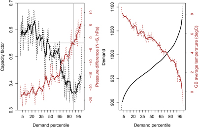
Figure 2 Left: Variation in GB average wind power capacity factor (black) and meridional pressure difference between two regions north and south of GB (hPa, red) with winter percentile of GB electricity demand, averaging over 1% bins (dashed) and 5% bins (solid). The pressure difference during the minimum wind power is highlighted by the grey lines. This pressure difference is used as a proxy to represent the larger scale pressure field over the North Atlantic (see section 4.1 for details). Right: Variation in electricity demand (GWh, black) and GB average temperature (∘C, red) with percentile of winter electricity demand.
Download figure:
Standard image High-resolution imageThe same relationship is seen when wind power is averaged across both onshore and offshore regions separately, across different regions of GB (North-west, North-east, South-west and South-east) and when calculating wind power using observed rather than reanalysis wind speeds (figure 3, and figures 8 and figure 10 in supplementary material). The demand–wind power relationship is therefore largely insensitive to the spatial distribution of turbines across GB. Across all demand conditions, average offshore wind has a capacity factor 15–25 percentage points higher than onshore wind, because of higher wind speeds offshore [19] (figure 3). Although the reduction in capacity factor with increasing demand is similar for onshore and offshore regions (reducing by ∼0.2), the percentage decline is smaller offshore than onshore, due to the greater magnitude of offshore wind power. For example, onshore wind power nearly halves whilst offshore wind power reduces by less than a third. In addition to wind power being lower onshore, during higher demand conditions, it is more frequently lower (figure 1, lower row).

Figure 3 Variation in average GB onshore (brown) and offshore (blue) wind power capacity factor with winter percentile of GB electricity demand. Capacity factors are presented as rolling 5% demand bin means. The 10th and 90th percentile capacity factors for each demand bin and each region are given (dashed).
Download figure:
Standard image High-resolution image4.1. The role of weather patterns
In the extra-tropics, large scale weather patterns in the lower atmosphere play a dominant role in shaping the weather experienced at the surface. The important weather features, such as low and high pressure systems, can be identified from a surface pressure field adjusted for the height of any topography. This is referred to as mean sea level pressure (MSLP). We therefore compare the average MSLP field during different demand conditions. Two demand categories are defined: low and high demand, representing the lower and upper 5% of winter demand days respectively, each containing 90 days. On average, a low or high demand day would be expected to occur two to three times per winter (only considering work days).
During low demand in winter, high pressure is centred over France and Spain, with low pressure centred over Iceland on average (figure 4). This stronger than average pressure difference across the North Atlantic, resembles the positive phase of the NAO. Associated with this pattern are generally stronger westerly winds (winds from west to east) and higher temperatures [20]. The air temperature across GB is over 3 ∘C higher than normal and wind power is often >20% above normal, with capacity factors ∼0.5 onshore, and >0.7 in many offshore regions.
In contrast, during high electricity demand, high pressure extends from Russia and Scandinavia across GB on average, with anomalously high pressure in northern Europe and anomalously low pressure in southern Europe (figure 4). These negative NAO type conditions typically produce colder, calmer conditions in northern Europe [20]. Cold easterly winds (winds from east to west) cause GB temperatures to fall below freezing and wind power is lower than average across all of GB (onshore capacity factors are typically <0.4, whilst offshore >0.5). Greatest reductions in wind power are seen over Scotland (>30% lower than average). The third column in figure 4 will be discussed in section 7.
The reduction in wind power with increasing demand in winter can therefore be explained by variations in the atmospheric pressure pattern over north-western Europe. A proxy for this field is the north-south (meridional) pressure difference over GB (red line, figure 2 left). This is calculated by averaging the mean sea level pressure over the two regions shown in figure 4, upper left (northern region: 27∘W–21∘E, 57∘N–70∘N, southern region: same longitudes, 38∘N–51∘N) and then subtracting the southern pressure from the northern pressure. A positive difference implies generally easterly winds, and a negative difference westerly winds. The greater the magnitude of the pressure difference, the stronger the resultant winds. The reduction in wind power with increasing winter demand seen in figure 2 is consequently associated with a weakening of both the meridional pressure difference and the westerly winds. Minimum average wind power occurs when there is little pressure difference (grey lines, figure 2), associated with high pressure sat directly over GB [16]. The upturn in wind power during higher demand is associated with a reversed and strengthening meridional pressure difference, and strengthening easterly winds.
Average air density over GB increases as demand in winter increases, due to a reduction in temperature and an increase in pressure. However the impact of density changes on the wind power–demand relationship is minimal. Using constant density would only over-estimate the reduction in wind power between higher and lower demand in winter by approximately 3%.
5. High electricity demand
To better understand the spatial and temporal variation of wind power during high demand days, we determine the dominant weather patterns during high demand and their respective wind power availability. K-means clustering [21] is applied to the mean sea level pressure fields of all high demand days. This is repeated 100 times to ensure that the cluster number chosen and the resulting cluster centroids are robust (see section 9.3 in the online supplementary material for further details). Four clusters are found to adequately represent the variability in pressure seen and are shown in figure 5.

Figure 4 Mean of MSLP, (mb, top), 2 m temperature (∘C, 2nd row), temperature anomaly (∘C, 3rd row), wind power capacity factor (%, fourth row) and wind power capacity factor anomaly (% difference from climatology, bottom) during low (left column), high (middle column) and peak (right column) GB electricity demand, between 01/01/1979 and 31/03/2013. ERA-Interim pressure and temperature data are used [18]. Anomalies are relative to the winter climatology (the long term average). The gray boxes in the upper left panel show the regions over which the surface pressure is averaged prior to calculating the meridional pressure difference.
Download figure:
Standard image High-resolution image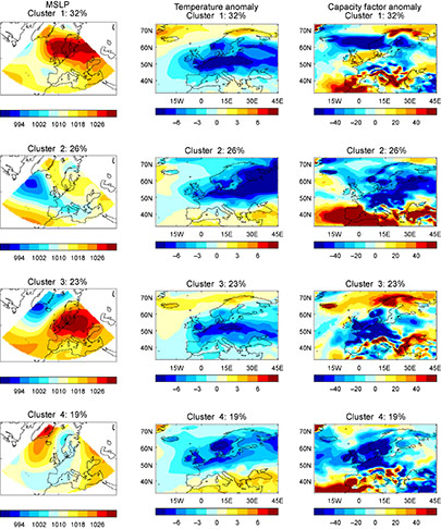
Figure 5 The cluster centroids over high demand days (MSLP, hPa, left column). The average 2 m temperature anomaly (∘C, middle column) and wind power capacity factor anomaly (% difference from climatology, right column) when averaged across all days in each cluster. Anomalies are relative to the winter climatology from 01/01/1979–31/03/2013. This cluster set is the set most representative of the bootstrap, see section 9.3 in the online supplementary material for details.
Download figure:
Standard image High-resolution imageAlthough individually distinct, the four weather patterns show that high pressure in the region plays an important role in generating high electricity demand in GB, as seen previously [16]. Each cluster has a similar occurrence frequency (ranging from 19%–32% of high demand days). High pressure is found over Scandinavia/Scotland (clusters 1 and 2), over central and northern Europe (cluster 3) and over Greenland and the North Atlantic (cluster 4), causing the advection of cold air over GB by easterly, south-easterly or northerly winds respectively.
During each high demand weather type, anomalously low temperatures are found across GB, with daily average temperatures often below freezing (figure 5, and figure 13 in the online supplementary material). This is expected, given the strong anti–correlation between electricity demand and temperature in winter [8]. However, spatial wind power availability differs across the weather types. For example, the strong north-south pressure difference over GB in cluster 1, gives wind power 20% higher than normal over most of England and Wales (capacity factor >0.4 onshore and >0.7 offshore). In contrast, a high pressure over Greenland and weak pressure over GB (cluster 4), gives wind power at least 40% below normal (capacity factors of <0.3 on land and <0.5 offshore).
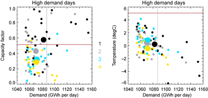
GB average wind power can vary across days with the same weather type (figure 6, left), reflecting the daily variation in both the pattern and its magnitude. Even with this variation it is clear that high demand days with wind power above the winter average are predominantly generated by the Scandinavian high and Atlantic low pressure patterns (clusters 1 and 2 respectively, see points above the red line). In contrast, the central European and Greenland high pressure patterns predominantly give daily capacity factors below the winter average (clusters 3 and 4 respectively).
Figure 6 Daily electricity demand and GB mean wind power capacity factor (left) and mean 2 m temperature (right) during high demand days. Each day is coloured by its MSLP cluster number (see figure 5). The mean properties for each cluster are indicated by a large circle. The vertical grey line defines the lower boundary of the peak demand days and the horizontal red lines mark the winter average wind power capacity factor (left) and temperature (right).
Download figure:
Standard image High-resolution image
6. The wider European picture
The weather patterns that bring low temperatures and high demand to GB, also cause anomalously low temperatures across many parts of Europe, both on average, and during individual types (figures 4 and 5 respectively). This is particularly true for the northern half of Europe where temperatures can be 6 ∘C below the winter average. Given the strong relationship between electricity demand and temperature in many European countries [7], high energy demand is therefore likely in neighbouring countries during high GB demand.
The majority of Europe also experiences below average wind power during high GB demand on average (figure 4, middle column, bottom row). Many countries have onshore wind power capacity factors <0.2, 20% or more lower than normal. Spain and Portugal are the exception, with much higher wind power than normal (>40% higher), although capacity factors are still only ∼0.2 onshore and ∼0.4 offshore. The anti-correlation between the wind field of GB and Iberia [22] is explained by the dipole response of the wind field to the NAO [14, 23].
Considering individual weather types, during windy, high demand days in GB, the North Sea, northern Germany and Denmark also have above average wind power, as these regions also sit between the two pressure centres (cluster 1, figure 5). However when GB has below average wind power (clusters 2–4), the majority of mainland Europe also has below average wind power (capacity factors <0.2). The main exception is the Iberian Peninsula during cluster 2, where capacity factors >0.3 (figure 13 in the online supplementary material).
7. Peak electricity demand
Peak demand days are of great interest to the energy industry. By their nature they are rare. Here we define peak demand as the top 1% of winter GB demand days, representing 18 days over the 34 year period. With this definition, a peak demand day would be expected to occur on average once every other winter (only considering work days). It is recognised that the sample size is small, but it is worthy of consideration for analysis because of the importance of days with the very highest demand.
The average MSLP pattern associated with peak electricity demand in GB is similar to that during high demand, but more intense (figure 4, right column). The reversed pressure difference is stronger (figure 2), resulting from higher pressure over Scandinavia and deeper pressure over south-western Europe. Strengthened easterly winds give rise to temperatures below −3 ∘C across GB and near average wind power.
The full range of high demand weather types are also seen during peak demand (figure 6, see points to right of grey vertical line), giving a wide range of average GB wind power, from very low (cluster 4, capacity factor of ∼0.1) to very high (cluster 1, capacity factor of ∼0.8). In this limited sample, half of the peak demand days have wind power above the winter average. The spike in wind power during peak demand seen in figure 2, is therefore explained by the higher percentage of cluster 1 type days. Interestingly, over this period the very highest demand appears to occur when temperatures are very low and wind power is very high, associated with strong easterly winds (cluster 1, figure 6). This suggests that either the higher wind speed directly increases demand, or the higher wind speeds are needed to bring larger quantities of cold air over GB, causing the very low temperatures and consequent very high demand. The former would support the use of a wind chill factor in peak electricity demand estimation, as used by National Grid [24].
Of particular concern is low wind power availability during peak demand. Cluster 4 is therefore of interest as the Arctic air flow can generate very low temperatures and very low wind power. During the 18 peak demand events investigated here, only 3 days have this weather type, all of which occurred during December 2010 (three yellow points, figure 6). During these days, wind power availability was very low both onshore and offshore (capacity factors <0.2). The relatively small number of years considered here limits our estimation of the likelihood of such peak demand events. An improved estimation could be made by assessing the likelihood of such weather types in a longer historical record or using large ensembles of model simulations.
8. Discussion
The availability of wind power during different electricity demand conditions in Britain is analysed between 1979 and 2013. We use daily observations of total GB demand and estimate wind power availability using reanalysis wind speeds and an idealised wind power model.
For the majority of the year, as demand increases, average available wind power also increases. However in winter, average wind power reduces by a third between lower and higher demand. This winter relationship is shown to be driven by the large scale weather patterns affecting Northern Europe. The change from predominantly strong, warm, westerly winds, to colder, calmer, easterly winds explains the reduction in wind power supply as demand increases. However, contrary to what is often believed, during high demand we find a modest recovery in average wind power, which is associated with a reversed north-south pressure gradient and the building of high pressure to the north of GB.
These average relationships hide considerable daily variability, where for a given demand, a wide range of wind power availability is possible. We find that during high and peak demand, a range of high pressure weather types generate similarly cold conditions over GB, but varying wind power supply. Approximately one-third of high demand days have wind power above the winter average, and two-thirds below. However, in our limited sample of peak demand days, although days do exist with very little onshore and offshore wind power, half of days have above average wind power, due to more days with strong easterly winds.
The characterisation of the relationship between electricity demand and wind power supply in Britain, should help both in the short term management of the energy system and in longer term planning. Wind power and demand are currently estimated using short term weather forecasts and demand and supply models. Uncertainty in the forecast of the proportion of demand met by wind power relates to both the accuracy of the weather forecast and the validity of the demand and generation models. Our analysis helps to explain the varying contribution of wind power and should help operational managers better interpret forecast information. For example, the range in possible wind power availability for a given demand can be reduced if the weather type is known.
Here we show that wind power can contribute to the supply mix during high and peak demand. The relationship is complex such that certain weather types provide good wind power, whilst others limit availability. The spatial distribution of wind power availability varies across these weather types, indicating that a spread of wind turbines across GB would maximise the average availability of wind power during high demand. In addition, the percentage reduction in wind power supply with increasing demand is lower offshore than onshore, suggesting offshore wind power is better placed to aid security of supply. This analysis highlights the risk of wide-scale high electricity demand and low wind power days across many parts of Europe, associated with large scale high pressure systems. Neighbouring countries may therefore struggle to provide additional capacity to GB when its demand is high and its wind power low.
Having identified the weather types important for the security of electricity supply in GB, such a classification will allow an assessment of their predictability on a range of timescales and also of possible changes in a changing climate.
Acknowledgments
This work was supported by the Joint UK DECC/Defra Met Office Hadley Centre Climate Programme (GA01101) and the European Climatic Energy Mixes (ECEM) project. ECEM is part of the Copernicus Climate Change Service and is being implemented by the European Centre for Medium-Range Weather Forecasts (ECMWF) on behalf of the European Commission (2015/C3S_441_Lot2_UEA). We thank National Grid for providing their demand data and the following people for useful discussions: David Lenaghan and Jeremy Caplin (National Grid), Robert Sanford (BEIS) and Doug Smith, Philip Bett, Julia Roberts, Nicky Stringer and Robin Clark (Met Office). We thank both reviewers for their helpful comments. Reproduced with the permission of the Controller of Her Majesty's Stationery Office.