


Abstract
Recent studies indicate that the glaciers and ice caps in Queen Elizabeth Islands (QEI), Canada have experienced an increase in ice mass loss during the last two decades, but the contribution of ice dynamics to this loss is not well known. We present a comprehensive mapping of ice velocity using a suite of satellite data from year 1991 to 2015, combined with ice thickness data from NASA Operation IceBridge, to calculate ice discharge. We find that ice discharge increased significantly after 2011 in Prince of Wales Icefield, maintained or decreased in other sectors, whereas glacier surges have little impact on long-term trends in ice discharge. During 1991–2005, the QEI mass loss averaged 6.3 ± 1.1 Gt yr−1, 52% from ice discharge and the rest from surface mass balance (SMB). During 2005–2014, the mass loss from ice discharge averaged 3.5 ± 0.2 Gt yr−1 (10%) versus 29.6 ± 3.0 Gt yr−1 (90%) from SMB. SMB processes therefore dominate the QEI mass balance, with ice dynamics playing a significant role only in a few basins.
Export citation and abstract BibTeX RIS

Original content from this work may be used under the terms of the Creative Commons Attribution 3.0 licence. Any further distribution of this work must maintain attribution to the author(s) and the title of the work, journal citation and DOI.
1. Introduction
The glaciers and ice caps of the Queen Elizabeth Islands (QEI), Canada cover an area of 105 000 km2, which represents 25% of the Arctic land ice outside Greenland (Lenaerts et al 2013, Van Wychen et al 2014). This region is divided into eight major ice caps and ice fields: 1) Northern Ellsmere Icefield (NEI), 2) Agassiz Ice Cap, 3) Prince of Wales Icefield (POW), 4) Devon Ice Cap (DIC), 5) Müller Ice Cap, 6) Steacie Ice Cap, 7) Sydkap Ice cap, and 8) Manson Icefield (figure 1). Time series of time-variable gravity and altimetry data indicate that the mass loss from QEI increased significantly to an average of 39 ± 9 Gt yr−1 for the time period 2004–2009, mostly the result of ice melt by warmer surface air temperature (Gardner et al 2011). A combination of surface mass balance (SMB) output products from the Regional Atmospheric Climate Model Version 2 (RACMO-2) and in-situ observations suggest that the QEI was close to a state of mass balance before year 2000 and started to lose mass from enhanced runoff after 2005 at an average rate of 35 ± 18 Gt yr−1 for the time period 2005–2011 (Lenaerts et al 2013).
Complete mapping of 2012 ice velocity (Van Wychen et al 2014) suggested that the loss from ice discharge is small compared to enhanced runoff and less than 10% of the total mass balance (Gardner et al 2011, Van Wychen et al 2014, Short and Gray 2005, Van Wychen et al 2016). The Randolph Glacier Inventory (RGI 3.2) (Arendt et al 2012), however, indicates that about half of the QEI is drained by marine-terminating glaciers: 254 marine terminating glaciers drain an ice area of 48 360 km2 versus 4 284 land-terminating glaciers draining an area of 56 513 km2. Changes in ice dynamics of tide-water glaciers may play a strong role in the mass balance of the QEI. In Greenland, for instance, 40%–50% of the mass loss is driven by the flow of marine-terminating glaciers, with the rest of the mass loss being controlled by an increase in runoff (e.g Rignot et al 2008). It is therefore of interest to investigate the partitioning of the mass balance of the QEI glaciers and extend the current time series over several decades to understand how it has been evolving with time and identify the physical processes behind those changes.
Here, we present a comprehensive analysis of the tidewater glaciers in the QEI between 1991 and 2015, including Devon Ice Cap, one of the largest contributors to ice discharge in this region, hence significantly expanding upon recent time series (Van Wychen et al 2016). We combine ice velocity from satellite data with ice thickness data from NASA's Operation IceBridge (OIB) from year 2012 and 2014 and surface mass balance (SMB) output products from RACMO-2.3 to determine the mass balance of the QEI, its temporal evolution over the last 25 years, and the exact partitioning of the mass loss between ice dynamics and surface mass balance processes, which has never been directly measured before on such time period. We conclude on the relative importance of ice dynamics in the overall mass budget of the QEI over the last 25 years.
2. Data and Methods
2.1. Ice discharge
We use Synthetic Aperture Radar (SAR) and optical data from the Japanese L-band sensor ALOS/PALSAR radar satellite (23.6 cm radar wavelength) collected between 2006 and 2011, the Canadian RADARSAT-1 data acquired in C-band (5.6 cm radar wavelength) between 2000 and 2004, the European ERS-1 C-band from 1991 (9 and 12 days repeat cycles), Sentinel 1-a C-band for winter 2015–2016, and the US Landsat 7/8 satellites from 2000 to present (satellite tracks are shown figure S17). A speckle tracking algorithm (Michel and Rignot 1999) for ALOS, ERS-1, RADARSAT-1, Sentinel 1-a and feature tracking for Landsat are used to calculate ice velocity. To enhance the surface features in the Landsat images, we use a 3 × 3 Sobel filter (Dehecq et al 2015). Cross-correlation is performed on image patches that are 350 m × 350 m in size on a regular grid with a spacing of 100 m for both SAR and optical images (Mouginot et al 2012).
We detect azimuth offsets in the SAR data caused by ionosphere perturbation (Gray and Mattar 2000). To remove these offsets we mask out the glacier areas and exploit the strong directionality of the streaks to form a 'streak model' (figure S1), which is calculated using a linear fit for each line of the azimuth offset map. This model is then removed from the data in the azimuth direction (see figure S2 for example). The global range and azimuth image offsets are calibrated using areas of presumed zero velocity (mountain outcrops, ice divides). We calculate a quadratic baseline to fit the data in the least square sense (Mouginot et al 2012). We mask out sea-ice areas using the SAR amplitude and Landsat images of the same time period. For rectification and geocoding, we employ the 1:250 000 version of the Canadian Digital Elevation Dataset (CDED), Level 1. Tracks are geocoded onto a polar stereographic grid with a central meridian at 45 °W and a secant plane at 70 °N at 100 m spacing. Velocity profiles are extracted along center lines of all major tidewater glaciers to assess changes in ice dynamics since 1991 (see Supplementary Online Material available at stacks.iop.org/ERL/12/024016/mmedia). We assemble yearly mosaic of ice velocity (figure S10 to S16) centered on winter and used later for ice discharge calculation (for example year 1991 corresponds to velocity from July 1991 to July 1992).
We estimate the error in ice speed by calculating the standard deviation of the signal in ice-free areas where ice motion should be zero. The RGI version 3.2 is used to delineate ice field and glacier boundaries (Arendt et al 2012). Errors are sensor dependent and vary from 3.6 m yr−1 for ALOS/PALSAR, 7.6 m yr−1 for RADARSAT-1, 20 m yr−1 for ERS1, 21 m yr−1 for Landsat-7 to 25 m yr−1 for Landsat-8 and 9 m yr−1 for Sentinel-1a. ERS1, RADARSAT-1 and Sentinel 1-a SAR data have larger errors due to lower image resolution and the stronger ionospheric perturbations.
Where ice thickness is available from OIB data along a glacier cross-section (e.g. Devon Ice Cap, Prince of Wales Icefield, Mittie glacier), we combine surface velocity with ice thickness to calculate ice discharge, D. The ice thickness was collected between 2012 and 2014 and has a nominal error of 20 m (Gogineni 2012). We calculate D as the mass flux passing through a flux gate close to the terminus of the glacier, converted into water equivalent using an ice density of 917 kg m−3. We combine the errors in velocity and thickness using the root of the sum of square to calculate the error in D. For glaciers with no thickness cross-section (ie 44%), we use OIB ice thickness at the centerline and interpolate across the glacier assuming a U shape-valley as in Van Wychen et al (2014). In this case, the error in ice discharge is calculated assuming that ice thickness is affected by a 12% error as in Van Wychen et al (2014).
Yearly D is obtained for 1991 through 2015. We fill data gaps using a linear temporal regression in D. These data gaps may include surge events, and so it is possible that we are underestimating the long-term ice discharge from the region. In total, we survey 80% of the marine terminating glaciers. When there is not enough data to calculate this regression, we extrapolate D using the closest non-surging value in time. We use the area of non-surveyed glaciers to calculate their ice discharge by scaling the median of the total D between 1991 and 2015 for each ice caps individually. We assume a conservative error of 100% for the scaled discharge. Table S1 summarizes the ice discharge for each glacier, the method employed, and the ice area of land-terminating and marine-terminating glaciers.
Additionally, we used Landsat images between 1970 and 2016 and amplitude images between 1991 and 2016 to determine the ice front position for Otto, Trinity, Wykeham and Belcher glaciers. The ice front was digitized manually using the Quantum GIS software.
2.2. Surface Mass Balance
We used the Regional Atmospheric Climate Model version 2.3 at 11 km spatial resolution (Ettema et al 2009) to quantify SMB over the past 25 years. Because RACMO overestimates ice areas under 1 000 m a.s.l (Lenaerts et al 2013), we use an hypsometry correction from a high-resolution DEM to correct SMB, runoff and precipitation. This DEM was obtain from the combination of 149 individual CDED DEMs derived from 1:60 000 aerial photographs acquired during the period 1950–1960 (Gardner et al 2011). The average value of SMB, runoff and precipitation for each DEM class is multiplied by the area at the corresponding elevation interval. The total SMB is then obtained by adding all the different classes together. The change in SMB due to the hypsometry correction averages 25% between 1958 and 2014. The uncertainty in SMB is calculated to be 30% in the QEI, with 10% from precipitation and 28% from runoff as it was determined by Lenaerts et al (2013). The average SMB for the period 1960–1990 is 1.2 ± 0.4 Gt yr−1 and the rate of mass loss for the period 2005–2011 is 32 ± 9 Gt yr−1, which is consistent with Lenaerts et al (2013). The total mass balance is calculated as the difference between SMB and D for individual glaciers and summed up over the entire icefields.
3. Results
The velocity maps clearly separate marine-terminating glaciers where ice speed increases continuously up to the ice front, from land-terminating glaciers where ice speed is maximal near the equilibrium line elevation and then decreases to zero at the ice front (figure 1). The mapping extends from the ice divides to the ice fronts, i.e. covers the entire ice masses. We observe significant fluctuations in glacier speed over time.
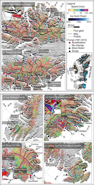
Figure 1 Flow speed of the QEI glaciers averaged between 1991 and 2015, color coded on a logarithmic scale, and overlaid on the CDED DEM in shaded relief. The survey domain is divided into 6 regions: (a) Northern Ellesmere Icefield, (b) Agassiz Ice Cap, (c) Axel Heiberg Islands, (d) Prince of Wales Icefield, (e) Devon Ice Cap, and (f) Sydkap Ice Cap and Manson Icefield. A full map of the QEI with CDED DEM in shaded relief is shown with the position of Nares Strait. Blue basins represent the drainage basins of marine-terminating glaciers and brown basins represent the drainage basins of land-terminating glaciers. Operation IceBridge (OIB) flight tracks are yellow, center flow lines are dash white, flux gates are yellow, and Randolph Glacier Inventory basin boundaries are black. Insets in (a), (d) and (e) show ice front positions of marine-terminating glaciers color coded from black, to blue and white from 1970 to 2015 for (a) Otto Glacier, (d) Trinity and Wykeham glaciers, and (e) Belcher Glacier. Glacier names are provided for major outlet glaciers. Red circles denote glacier acceleration. White circles denote no change in speed. Blue circles denote a slow down in speed during the period 1991 to 2015. Surging glaciers during the 1991–2015 time period are denoted with a black triangle.
Download figure:
Standard image High-resolution imageThe Northern Ellesmere Icefield (NEI) includes large-size marine-terminating glaciers on its western and northern flanks (Otto, Milne, Yelverton, M'Clintock and Disraeli) and land-terminating glaciers along its southern and eastern flanks that represent more than 60% of the ice area (16 871 km2, figure 1(a) and table S1). The ice discharge from NEI averaged 0.48 ± 0.08 Gt yr−1 between 1991 and 2000 (table S1). The discharge increased after 2001 to peak at 0.53 ± 0.12 Gt yr−1 in 2006 during the surge of Otto Glacier (table S1 and figure S5). Ice discharge then dropped to 0.31 ± 0.1 Gt yr−1 in 2015 due to a decrease in speed of most glaciers. Otto Glacier experienced a significant slow down between 1991 and 2015 with a frontal speed dropping from > 800 m yr−1 in 1991 to <50 m yr−1 in 2013–2015 (figure S5). After 2010, more than half of the ice discharge of NEI was driven by Yelverton and Milne glaciers with an average total of 0.15 ± 0.06 Gt yr−1 between 1991 and 2015 (table S1).
The Agassiz Ice Cap, between the POW and NEI, comprises a large number of marine-terminating glaciers that represents 8 844 km2 (40% of the ice area, figure 1(b) and table S1). The ice discharge was nearly constant between 1991 and 2000 with an average of 0.28 ± 0.05 Gt yr−1. An average mass flux of 0.5 ± 0.04 Gt yr−1 is calculated between 2005 and 2007 due to the combined surge of Parrish Glacier and Glacier 5 (figure S3 and table S1). The mass flux of 60% of the glaciers decreased during 2010–2015 compared to 1991–2010 (figure 3, figure S3, table S1). Cañon, Glacier 4, Dobbin and Tuborg Glaciers are the only ones that maintain a steady state regime during 2000–2015.
The POW is located in the central part of Ellesmere Island between 76 °N and 78 °N (figure 1(d)). The western part only includes land-terminating glaciers whereas the eastern part is drained by large marine-terminating glaciers that drain >60% of the total area (table S1). The ice discharge of POW averaged 1.6 ± 0.1 Gt yr−1 between 1991 and 2008 and increased by a factor of 1.5 since then. During the time period 2009–2015, D increased to 2.46 ± 0.4 Gt yr−1 (figure 3 and table S1). 83% of the glaciers slowed down or maintain a steady regime, however, so the increase in D was only due to the acceleration of two glaciers: Trinity and Wykeham (figure 2, figure 3 and table S1). Draining from a common basin, these glaciers flow several times faster than any other glacier in the QEI (figure 1). Their ice speed (figure 2) was stable in 1991–2009, accelerated by a factor of two to 1 200 m yr−1 for Trinity and 650 m yr−1 for Wykeham in 2015. Examination of the position of the ice fronts reveals a continuous retreat of Trinity Glacier since 1991 by 5 km (figure 2). The retreat amounts to 7.7 km since 1976 (figure 1(d)). Wykeham Glacier retreated 1.8 km between 1991 and 2015 and 4.2 km between 1976 and 2015. At present, the northern part of Wykeham ice front is no longer retreating (figure 2).
South of POW, on Sydkap Ice Cap and Manson Icefield (figure 1(f)), Sydkap Glacier ice discharge dropped from 0.04 ± 0.001 Gt yr−1 in 1991 to 0.02 ± 0.002 Gt yr−1 in 2010 and slightly increased to 0.05 ± 0.001 Gt yr−1 in 2015 (table S1). In contrast, we calculate a mass flux in 2000 of 0.9 ± 0.01 Gt yr−1 for Mittie Glacier, followed by a decrease to an average 0.02 ± 0.002 Gt yr−1 for 2003–2015. Similar abrupt changes in ice discharge are detected for Iceberg and Good Friday Bay glaciers on Axel Heiberg Islands in 1991 (figure 1(c) and S7).
Finally, the DIC is characterized by a dominance of marine-terminating glaciers (10 275 km2 vs. 4 722 km2 for land-terminating glaciers) (figure 1(e), 2). The discharge of the entire ice cap increased from 0.46 ± 0.1 Gt yr−1 to 0.53 ± 0.1 Gt yr−1 between 1991 and 2015. However the increase in D is within the uncertainty, so we cannot draw solid conclusions on the evolution of this sector. Belcher, South Croker Bay and Fitzroy are the fastest moving glaciers, with speeds of 300 m yr−1 at their calving fronts. Most glaciers have maintained a steady flow regime since 1991 and the increase in ice discharge is mainly due to the 50% acceleration of Belcher during this period (table S1, figure S6). North Croker Bay displays a significant slow down to zero frontal speed in 2015, which suggests that the glacier may have detached from the ocean or have become analogous to a land terminating glacier.
Overall, more than 60% of the ice discharge was measured for 9 years (outside interpolations and extrapolations) compared to the 5 years of recent studies (Van Wychen et al 2016), with crucial new data between 2004 and 2010. Importantly, our discharge results extend these studies further back in time from 2000–2015 to measurements between 1991 and 2016, which is important to draw conclusions about long term changes in ice dynamics. Differences in total surveyed ice discharge for common years results from the addition of Devon Ice Cap in our study, which is the second highest contributor to the total ice discharge and from differences in survey area. We estimate that Devon Ice Cap contributes an average 0.46 ± 0.01 Gt yr−1 discharge over 1991–2015, in agreement with Van Wychen et al (2012) for year 2009. The total ice discharge is on average 1.4 ± 0.5 Gt yr−1 higher than in Van Wychen et al (2016) for complete years (i.e. 2000, 2011, 2013, 2014 and 2015).
4. Discussion
The difference between surge and pulse type glaciers is defined by the velocity structure, and particularly in the region of initiation and propagation (Van Wychen et al 2016). As the definition of pulse-type glacier vary from study to study (e.g. Mayo (1978), Raymond (1987), Turrin et al (2014), Van Wychen et al (2016)) and because the difference between these two behaviors is not crucial in the calculation of the mass balance, surge and pulse type glaciers are both referenced as 'surge type' glaciers hereafter.
Among the 43 major glaciers surveyed in this study, 65% did not change speed or even slowed down. We detect 6 major surging glaciers: Mittie, Parrish, Dobbin, Good Friday Bay, Middle and Iceberg glaciers that were also documented in Copland et al (2003) and Van Wychen et al (2016). However, we report here new informations on the important increase in speed of d'Iberville, Glacier 9 and Glacier 11. The 300 m yr−1 speed of d'Iberville glacier in 1991 was three times higher than for the period 2000–2015. In 2007, Glacier 11 quadrupled its ice discharge from 0.01 ± 0.01 Gt yr−1 to 0.04 ± 0.01 Gt yr−1. Similarly, Glacier 9 increased its ice discharge to 0.2 ± 0.06 Gt yr−1 in 2006, which is 8 times higher than in 2000 and for the period 2010–2015. Evidence of surge features such as loop moraines, intensive crevassing or dramatic terminus position are lacking at this time for d'Iberville glacier in 1992. No such features were found on Glacier 11 and Glacier 9. Analysis of the thinning pattern would be necessary to draw conclusions on the changes in dynamics of these glaciers and to determine if it can be attributed to surge episodes. In total, however, the ice discharge from all these glaciers remains low, even after accounting for the surges and short term peak in D. The average D for D'Iberville, Dobbin, Parrish, Otto, Good Friday Bay, Iceberg, Mittie, Glacier 11 and Glacier 9 are, respectively, 0.02, 0.04, 0.04, 0.1, 0.1, 0.04, 0.1, 0.01 and 0.07 Gt yr−1 (average of errors across all surging glaciers is below 0.005 Gt yr−1). As a result of the surges that took place during the period 1991–2015, we estimate that D increased by 0.2 Gt/yr or 6%. The effect of surges and peak in ice discharge on the decadal mass balance of the glaciers is therefore small.

Figure 2 Ice dynamics of Trinity and Wykeham glaciers: (a) Ice velocity on a logarithmic color scale with Operation IceBridge (OIB) flux gate in green, Randolph Glacier Inventory basin outline in black, center flow line profiles in dotted white, and ice front positions from 1970 to 2015 color coded on a linear scale from black, to blue, and white; (b) ice discharge of Trinity and Wykeham glaciers colored by year from blue to green and red, with SMB (not corrected from hypsometry) in blue and reference SMB for the years 1960–1990 as an horizontal blue line. Speed changes between 1991 and 2015 along (c) and (d) center flow lines A-A' and B-B' and (e, f) across the flux gates C-C' and C'-C'' with (g, h) corresponding OIB ice thickness. Flow speed in (c–f) are also coded from blue, to green and red for the years 1992 to 2015.
Download figure:
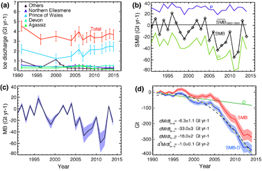
Standard image High-resolution imageIn total for QEI, we find that D decreased from 4.5 ± 0.5 Gt yr−1 in 1991 to 3.5 ± 0.5 Gt yr−1 in 2000 due to a decrease in flow speed of several glaciers (figure 3 and table S1). Between 2000 and 2015, D remained constant because the slow down of most glaciers was compensated by the speed up of Trinity and Wykeham glaciers. At the local scale, however, D is a significant component of the mass balance for Trinity and Wykeham glaciers. Both glaciers experienced the largest increase in ice speed of the entire archipelago. Analysis of the SMB record (figure 2) reveals that these glaciers were in balance between 1991 and 2008 with an ice discharge of 0.6 ± 0.02 Gt yr−1 (figure 2) versus a SMB of 0.83 ± 0.2 Gt yr−1. After 2008, the mass balance decreased from +0.25 ± 0.1 Gt yr−1 (i.e. a mass gain) to −1.0 ± 0.2 Gt yr−1. This increase in mass loss is due to a doubling in runoff production from 0.43 ± 0.02 Gt yr−1 to 0.83 ± 0.1 Gt yr−1 and a doubling in ice discharge from 0.6 ± 0.02 Gt/yr to 1.5 ± 0.1 Gt yr−1 after 2009. The increase in glacier speed tripled the mass loss caused by enhanced runoff alone. In total, these two glaciers contributed a 37% increase in total discharge from QEI since 2010 (figure 3). Yet, this is the only sector in QEI where changes in speed have had a significant impact on total mass balance.
During the time period 1991–2005, the QEI was losing mass at a rate of 6.3 ± 1.1 Gt yr−1 (figure 3). Ice discharge contributed 52% of the losses (3.4 ± 0.1 Gt yr−1 discharge vs 3.0 ± 1.1 Gt yr−1 from SMB). After 2005, the mass budget became strongly negative due to a significant increase in runoff that reduced SMB to −55.6 ± 16.6 Gt yr−1 in 2012 (figure 3(b)). During that time period, there was no trend in precipitation, which averaged 28 ± 2.9 Gt yr−1 (figure 3(b)). The loss due to ice discharge of 3.5 ± 0.2 Gt yr−1 therefore contributed only 10% of the total loss, i.e. the loss was dominated by enhanced runoff. This is consistent with previous studies over shorter time periods (Gardner et al 2011).
Figure 3 Mass budget of the Queen Elizabeth Islands (QEI), Canada from 1991 to 2015: (a) ice discharge for several icefields and for the entire survey domain. 'Others' includes Sydkap, Mittie and Axel Heiberg icecaps. Error bars are only shown for years with measurements. (b) total surface mass balance (SMB), runoff (R), precipitation (P), and reference SMB for the years 1960–1990 for the entire survey domain, (c) total mass balance (MB=SMB-D); (d) cumulative surface mass balance, ice discharge, and total mass balance for the entire survey domain. Mass balance trends for 1991–2005, 2005–2014 (yellow dashed line) and quadratic fit for 1991–2014 (black dashed line) are shown in (d).
Download figure:
Standard image High-resolution image
The transition in mass balance coincides with a marked increase in summer air temperature around year 2004 that has continued until present (Gardner et al 2011). In the period 2013–2014, runoff production decreased and SMB increased from −55.6 ± 16.6 Gt yr−1 to +8.2 ± 2.5 Gt yr−1. This pause in mass loss resulted from colder-than-average consecutive summers following the large melt event of 2012 (Tedesco et al 2015, Harig and Simons 2016). Over the entire time period 1991–2014, the mass loss averaged 16.0 ± 1.7 Gt yr−1, with an acceleration of 1.0 ± 0.1 Gt yr−2.
Interestingly, we can notice that mass balance estimates vary significantly with respect to the methods. Indeed, calculation from straight altimetry or gravimetry shows values of 27 ± 7 Gt yr−1 and 24 ± 6 Gt yr−1 for 2003–2010 (Nilsson et al 2015, Colgan et al 2014). This number are much lower than the 34 ± 13 Gt yr−1 from Gardner et al (2011) for 2004–2009 that are closer from the 35 ± 18 Gt yr−1 during 2005–2011 (Lenaerts et al 2013) and the 33.0 ± 3.0 Gt yr−1 during 2005–2014 from this study. Thus, it seems that the uses of an input-output method, with a surface mass balance model gives larger estimates than a mass balance derived only from altimetry or gravity.
To understand the evolution of marine-terminating glaciers in POW, it is essential to investigate their interaction with the surrounding ocean because the intrusion of warm ocean waters have the potential to melt ice in contact with it, undercutting the ice fronts and increasing iceberg calving (Motyka et al 2003, O'Leary and Christoffersen 2013, Bartholomaus et al 2013). Ocean currents along POW are driven by the inflow from Nares Strait (see figure 1 for location). Munchow et al (2011) report an increase in ocean temperature in Nares Strait after year 2007 which would suggests that ice melting by the ocean must have increased significantly around that time. Enhanced melting of the calving margins may have dislodged the glaciers from their stabilizing positions after 2010, when Trinity and Wykeham start to accelerate and increase their ice discharge significantly (table S1, figure 2). From these observations, we suggest that ice melting by the ocean must have started to increase prior to 2010. Details on the bathymetry, glacier bed topography, and ocean temperature in front of the glaciers are, however, lacking at this time to make any firm conclusions about the changes in this sector.
We find that 9 glaciers reduced their frontal speed to zero during the time period (figure S3 to S7), suggesting that they lost contact with the ocean, hence stopped calving, as they retreated to higher ground. Alternatively, these glaciers are surge type glaciers that transitioned to a quiescent phase. An analysis of Landsat-8 2015 images indicate that the glaciers were still all in contact with the ocean because we find no moraine deposit separating the ice front from seawater (figure S8). Hence, these glaciers remain marine terminating. We note, however, that most of them are rather thin at the ice front, and less than 100 m thick (figure S8). At this level of ice thickness, the driving stress is quite low, i.e. ice may not deform internally (Hutter 1982). Hence, these glaciers, while reaching the ocean, are more similar to land-terminating glaciers than to tidewater glaciers.
The mass loss of the QEI averaged over its 105 000 km2 area is 0.17 ± 0.05 m yr−1 water-equivalent (w.e) for the time period 1991–2014 (0.06 ± 0.02 m yr−1 for 1991–2005 and 0.34 ± 0.03 m yr−1 for 2005–2014). For comparison, Alaskan glaciers experienced a mass loss of 75 ± 11 Gt yr−1 for the time period 1994–2013 (Larsen et al 2015), i.e. an average loss of 0.7 ± 0.1 m yr−1 w.e over their 85 000 km2 area, or 4 times larger. Conversely, the mass loss of the Patagonia Icefields averaged 24.4 ± 1.4 Gt yr−1 between 2000 and 2012 (Willis et al 2012b), which corresponds to an average mass loss of 1.3 ± 0.1 m yr−1 w.e over their area of 21 000 km2, or 7.6 times larger than for the QEI. Hence, the average mass loss per unit area decreases markedly from low latitudes (Patagonia) to high latitudes (QEI). The QEI currently contributes more mass loss than Patagonia because of its larger area, but we posit that a change in global mean surface air temperature of 0.3 °C–0.5 °C for the period 2016–2035 as projected by the IPCC report (IPCC 2013) could potentially increase the mass loss of the QEI to reach the values observed in Patagonia, which is one order magnitude larger per unit area.
5. Conclusions
We present the largest time series of glacier velocity and mass balance for the Queen Elizabeth Islands, in Canada spanning from 1991 to 2015 with a complete velocity mapping at 100 m spacing. The acceleration of Trinity and Wykeham between 2010–2015 increased the ice discharge by 37% and accounted for 50% of the total ice discharge from the QEI to the ocean in 2015. Yet, even if ice discharge can play an important role at the basin scale, its contribution to the total mass loss from these icefields remains small. Similarly, glacier surges do not have a significant impact on the long-term mass balance of the QEI. The vast majority of the mass loss is controlled by SMB processes, mainly runoff. Prior to 2005, the rate of mass loss was low and controlled by ice discharge. After 2005, the mass loss increased markedly to transform the QEI into a major contributor to sea level change. With ongoing, sustained, rapid warming of the high Arctic, the mass loss of QEI should continue to increase significantly in the coming decades to century.
Acknowledgments
This work was performed at the University of California Irvine and at Caltech Jet Propulsion Laboratory under a contract with the National Aeronautics and Space Administration Cryosphere Science Program (NNX13AI84A, NNX14AN03G, NNX14AB93G). Velocity data from QEI are available upon request from the authors and will be posted at the National Snow and Ice Data Center, Boulder, Colorado.