

Abstract
We quantify the importance of early action to tackle urban sprawl. We focus on the long-term nature of infrastructure decisions, specifically local roadways, which can lock in greenhouse gas emissions for decades to come. The location and interconnectedness of local roadways form a near-permanent backbone for the future layout of land parcels, buildings, and transportation options.
We provide new estimates of the environmental impact of low-connectivity roads, characterized by cul-de-sacs and T-intersections, which we dub street-network sprawl. We find an elasticity of vehicle ownership with respect to street connectivity of –0.15—larger than suggested by previous research. We then apply this estimate to quantify the long-term emissions implications of alternative scenarios for street-network sprawl. On current trends alone, we project vehicle travel and emissions to fall by ∼3.2% over the 2015–2050 period, compared to a scenario where sprawl plateaus at its 1994 peak. Concerted policy efforts to increase street connectivity could more than triple these reductions to ∼8.8% by 2050. Longer-term reductions over the 2050–2100 period are more speculative, but could be more than 50% greater than those achieved by 2050. The longer the timescale over which mitigation efforts are considered, the more important it becomes to address the physical form of the built environment.
Export citation and abstract BibTeX RIS

Original content from this work may be used under the terms of the Creative Commons Attribution 3.0 licence.
Any further distribution of this work must maintain attribution to the author(s) and the title of the work, journal citation and DOI.
Changes were made to this article on 20 March 2017. The supplementary data link in the pdf was corrected.
1. Introduction
'Street-network sprawl' is the characteristic of urban sprawl defined strictly by properties of the location and interconnectedness of roads [1]. Street-network sprawl is characterised by low connectivity in road networks, which is associated with car-oriented transport as well as segregated land-uses and low-density residential development [10]. After decades of steadily declining road connectivity, recent trends in the USA show a major turnaround toward less sprawl. Since the mid-1990s, new urban road construction has become increasingly grid-like, with quantitative measures of connectivity recently returning to values typical of 1960s neighborhoods [1].
A turnaround in street-network sprawl is significant in part due to its importance for vehicle travel and for the associated emissions. In the USA in 2011, gasoline consumption for personal vehicle use accounted for 21% of CO2 emissions from fossil fuel combustion [33, p 10]. A large body of empirical evidence links sprawl with greater vehicle travel, energy consumption, and greenhouse gas emissions [10, 30]. These studies highlight the role of the street network itself—among other related dimensions of urban form such as density, commercial and residential mix, and public transit—as a particularly strong determinant of car ownership and travel behavior [16, 24, 29].
While major energy investments such as coal-fired power plants have capital turnover time scales on the order of a few decades, and some other infrastructure such as large dams may last for half a century, the locations chosen for roads have proven to be essentially permanent decisions among modern civilizations, outlasting buildings and large technological, economic, and social shifts. For this reason, our focus on metrics and policies related explicitly to road networks is particularly relevant to multi-decade and long-term climate policy. Over shorter time scales, initiatives related to more malleable infrastructure such as the energy efficiency of vehicles and buildings may appear more important.
In this paper, we quantify the shift that has already happened in street-network sprawl and estimate its significance for greenhouse gas emissions through its effect on vehicle usage. We find a larger impact of street-network sprawl on travel behavior than previous studies suggest. We subsequently present our main contribution, which builds on travel behavior studies and historical estimates of road connectivity to project future scenarios of greenhouse gas emissions. We consider what the turnaround in street-network sprawl implies for the future if the same trend continues, and also what a more aggressive shift could accomplish, for instance through concerted policy explicitly targeting the connectivity of roads built in new developments. We project a larger greenhouse gas mitigation effect than expected from other proposed transportation-sector policies.
After further elaborating on the importance of original decisions about road layout in section 1.1, sections 1.2 and 1.3 explain our measures of connectivity and how they are quantitatively related to vehicle emissions. Section 2.1 describes our methods for generating improved estimates of this relationship, based on nationwide road network data in the US. Section 2.2 discusses our methods for quantifying emissions impacts in terms of three possible scenarios for future trends in road network construction. Our results are presented in section 3, and section 4 concludes.
1.1. The significance and persistence of road networks
Across US urban regions, car ownership rates and per capita annual distances driven on roads vary considerably. As mentioned above, a range of studies investigates and quantifies the link between physical urban form and car use (see [10, 29] for meta-analyses). In places where the roads are dominated by cul-de-sacs and three-way intersections, rather than a more grid-like arrangement, more cars are needed and those cars are driven more, even after controlling for other aspects of urban form such as distance to transit, distance to downtown, and population density.
There are theoretical grounds to believe that this association is driven by features of the built environment, and the connectivity of the street network in particular, rather than the other way around. A gridded street network with high connectivity reduces the ratio of network distance to Euclidean distance, which reduces walking distances and tends to be more attractive to pedestrians. It is also difficult for public transportation to penetrate regions of urban sprawl characterized by low-connectivity roads both because their low population density makes mass transit inefficient, and because walking routes to potential transit stops are long and indirect. In turn, limited pedestrian access means that regions of street-network sprawl are unable to densify or to accommodate a system of distributed, close-by commercial services, even in the face of migration or changing costs.
Moreover, households in low-connectivity, car-oriented neighborhoods tend to need large dwellings because many of the services provided collectively outside the home in dense developments must instead be provided separately by domestic capital in each household [21]. Thus, developments with low-connectivity road networks are less likely to develop local restaurants, shops, laundromats, public swimming pools, gyms, and so on, which might otherwise facilitate a shift to denser residential dwellings. In summary, areas with low-connectivity road networks have a limited ability to adapt in the face of changing fuel prices, carbon taxes, or even amenities in nearby developments.
Above all, the relationship between street-network sprawl and other outcomes of urban form is underlain by the permanence of the street network. This persistence comes in part from the difficulty of coordinating across many landowners, once adjacent land has been subdivided, and the high cost of re-aggregating or appropriating private land. Thus, while buildings can be replaced, and other commercial and public infrastructure can respond to changing needs, tastes, and prices, residential roads tend to remain where they were first placed. The rebuilding of roads in their original locations following complete devastation in London (1666) and San Francisco (1906) were dramatic demonstrations of the persistence of road and property boundaries [13, p 227].
Because the responsiveness of building design and commercial and public infrastructure to any future changes in social and economic context is constrained by the road network properties once they are cemented, the road network itself may be seen as a cause of longer-term outcomes. Recent patterns and future trends of road network connectivity in new construction are therefore most significant for long-term (multi-decade) transport efficiency and GHG emissions, although they may have strong implications also for other more immediate and long-run outcomes including cardiovascular health [17]. As the Intergovernmental Panel on Climate Change notes, the long-lived nature of the built environment tends to lock in energy consumption and emissions once urbanization occurs [30].
1.2. Measuring street-network sprawl
We recently built a high spatial resolution time series of road network connectivity for the USA over the past century [1], which conceptualizes and quantifies street-network sprawl by classifying every street intersection, or node, into one of three types, according to its network-theoretic degree. Dead ends are considered an intersection of degree 1, three-way intersections are assigned degree 3, and we treat all intersections with four or more connected road segments as degree 4 (denoted 4+).
Figure 1 shows this classification applied to two sample neighborhoods. We refer primarily to two aggregate measures useful for describing geographic regions; these are the mean nodal degree,  , which is the average degree of nodes in a geographic unit, and the fraction D4+ of nodes with degree 4+. The highest connectivity developments are gridded street networks, typical of the early 20th century US construction that now constitutes urban cores. These neighborhoods have
  , while at the other extreme the archetypal suburban sprawl consists mostly of degree 1 and 3 nodes.
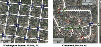
Figure 1 Nodal degrees evaluated for a highly connected (gridded) neighborhood and one characterized by dead ends. The Washington Square neighborhood, close to downtown Mobile, Alabama, has a mean nodal degree of 4.0, while the Claremont neighborhood about 10 miles away has a mean nodal degree of 2.15. Image source: Google Earth.
Download figure:
Standard image High-resolution image1.3. Existing estimates of car use elasticity
Most of the empirical studies included in recent meta-analyses [10, 29] measure street-network connectivity using D4+ or a related measure, nodal density (i.e. intersection density), with one study using the fraction of deadends. Ewing and Cervero [10] provide a useful benchmark, calculating a weighted average per capita vehicle distance traveled elasticity of −0.12 with respect to D4+, and an identical elasticity with respect to nodal density. Table 1 lists existing estimates of the elasticities of vehicle use with respect to road network connectivity from the two meta-analyses mentioned above.
Table 1. Previous studies of elasticity of vehicle distance traveled with respect to street connectivity metrics. Adapted from table 2 in Salon et al [29] and table 3 in Ewing and Cervero [10].
| Study | Elasticity | Nodal measure | Connectivity metric |
|---|---|---|---|
| Boarnet et al (2004) | 0.19 | density | Total intersection density near home |
| −0.06 | density | 4-way intersection density near home | |
| Bento et al (2003, 2005) | −0.07 | density | Road density (lane-miles per square mile) |
| Chapman and Frank (2004) | −0.08 | density | Intersection density near home |
| Ewing and Cervero (2010) | −0.12 | density | Intersection or street density (6 studies, none controlling for self-selection) |
| −0.12 | degree | Percent 4-way intersections (3 studies, 1 controlling for self-selection) | |
| Fan and Khattak (2008) | −0.26 | degree | Percent of road ends that are intersections rather than dead ends |
| Cervero and Kockelman (1997) | No effect | degree | 4-Way intersections HH VMT, all purposes |
| −0.59 | degree | 4-Way intersections HH VMT, non-work | |
| 0.18 | degree | Quadrilateral blocks HH VMT, all purposes | |
| 0.46 | degree | Quadrilateral blocks HH VMT, non-work |
The theoretical link between street-network connectivity and travel behavior is well-established, and supported by the empirical studies discussed above. However, most empirical work on the link between urban form and street-network design focuses on certain measures, particularly nodal density (nodes km−2) or the almost-equivalent measure of block size, that do not strictly measure connectivity. While there is likely a close relationship between nodal degree and nodal density, the latter measure is strongly mediated by the scale of the analysis (larger areas will include more parks and other undeveloped spaces), and does not distinguish between a cul-de-sac or a 4+ node. Nodal density also conflates two conceptually separate aspects of urban form, population density and street-network connectivity. Therefore, our analysis focuses on nodal degree as our preferred measure of street-network sprawl.
Moreover, existing studies may not fully identify the causal relationship running from the street network to car ownership and use. For example, an ordinary least squares regression, even if controlling for variables such as income, may suffer from an endogeneity bias if it does not account for an unmeasured (and possibly unmeasurable) variable that affects both street-network connectivity and car use independently. As an example, a coordinated public policy or pro-environmental political attitudes might promote connected streets, while simultaneously but independently encouraging alternatives to the private car. Therefore, in order to overcome the endogeneity bias, our preferred estimates use an instrumental variables approach [36] which, under assumptions explained below, allows us to evaluate the strength of a unidirectional causal component of the overall relationship between street connectivity and car use. The justification and methods for the instrumental variable estimates are considered in detail in section 2.1.2. Before that, we discuss our overall approach and choice of dependent variable.
2. Methods and data
Our approach to estimating vehicle emissions based on scenarios of future road-network connectivity can be separated into two steps, diagrammed in figure 2. First, we describe in section 2.1 links 3 and 4 between road network connectivity and car use. Second, in section 2.2 we develop several scenarios of future trajectories for road network properties in the US (link 1) based on our previous work, and we use existing projections for housing growth in order to estimate future car use, and from it, vehicle emissions (link 5).
2.1. The road network → car use relationship
The link between road‐network connectivity and car use is the most abstract of those shown in figure 2, and requires new econometric identification and estimation to corroborate and improve on the existing estimates cited in table 1. Our method focuses on variation at the scale of census block groups and uses the number of vehicles per household as a proxy for vehicle travel. We use a 2013 cross-section of nodal degree values covering all urban block groups in the USA4, along with census data on car ownership.
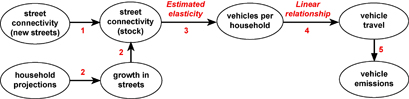
Figure 2 Process for predicting the impact of road network changes on vehicle emissions.
Download figure:
Standard image High-resolution image2.1.1. Vehicles per household as a measure of vehicle travel
Ideally, we would directly estimate the elasticity of vehicle distance traveled with respect to differences or changes in road network connectivity. This relationship across US states is shown in the top row of figure 3 for total urban annual per capita vehicle distance traveled. The distribution of state values suggests that states with higher-connectivity roads, as measured by  (left) and D4+ (right), exhibit lower vehicle travel per capita5. However, these data [34] are available only at the state level, and include commercial and freight vehicles in addition to household travel.

Figure 3 The bivariate relationship between two measures of car use and our two metrics for road-network connectivity. Top row: US state-level data for total motorized distance traveled on urban roads show a weak negative association with network connectivity. The solid line is a non-parametric (kernel-weighted local polynomial smoothed) fit. The high-travel outlier is Alabama. The right-most 'state' is actually the District of Columbia; however, removing these two observations does not significantly affect the estimate (dashed line) within the abscissa range of other states. Shaded areas show 95% confidence intervals. Bottom row: Census block groups with higher connectivity tend to house residents with fewer vehicles per household. Nonparametric (as above) estimates of the bivariate relationship at these high resolutions are shown by the purple lines, with shaded envelopes indicating 95% confidence intervals. Linear parametric plots agree closely and are shown in green. In our calculations we include all 72 893 urban block groups that contain more than 50 intersections but, for clarity, the figure shows only a random sample of 10 000 of these block groups.
Download figure:
Standard image High-resolution imageBecause we are interested in the local-scale impact of street connectivity, our estimates use block group level data. Comprehensive data on household urban vehicle travel are not available for such small geographic areas. Instead, our candidate proxies for vehicle travel are household vehicle ownership and commute mode share, both available from the American Community Survey. We consider the vehicle ownership variable to be the most natural proxy for household urban vehicle travel, not least because most household vehicle use is for trips other than commuting. Thus, of the measures available from the American Community Survey, the total number of cars chosen by households has a better theoretical link with overall car use than the measures which focus only on commuting.
Empirically, both vehicle ownership and commute mode share are highly correlated with vehicle travel. Using data from the National Household Travel Survey [12], we find that the log of vehicle miles traveled has a correlation of 0.28 with the share of commutes by driving, and 0.35 with the number of vehicles per household (and 0.42 with the same variable in log form). These correlations are at the household level, using the provided survey weights. Below it will be important only to assume that the relationship between the number of vehicles per household and mean distance traveled is roughly linear. Figure 4 shows that this is, as a correlational claim, an excellent assumption. The great majority of households have fewer than five vehicles, and for these households, the number of vehicles is nearly perfectly correlated with the mean vehicle distance traveled. While there are undoubtedly a host of factors which codetermine vehicle ownership and vehicle travel, we hereafter focus our causal identification on the link between urban form and vehicle ownership, and based on figure 4, assume similar fractional changes in vehicle ownership.

Figure 4 Number of vehicles per household versus distance traveled. Using data from the NHTS, the histogram shows the distribution of the number of cars owned by households. Mean distances traveled are shown as dots (with 95% confidence intervals as vertical bars). The blue line is a fit to the means, weighted according to their confidence. (A fit to the medians or a regression fit to the disaggregate houshold-level data show similar linear relationships for households with fewer than five vehicles.) The grey 'violin plots' show kernel density estimates of household vehicle distance traveled. For clarity, the long right (top) tails of the violin plots are truncated for households with many cars. We summarize these results by saying that for the vast majority of households, there is a closely linear relationship between vehicle number and mean distance traveled.
Download figure:
Standard image High-resolution imageThe lower panels in Figure 3 show distributions of mean degree  and D4+ at the scale of block groups, plotted against the average number of vehicles per household, taken from the 2007–2011 American Community Survey. There is a clear linear relationship between higher connectivity streets and fewer vehicles per household. The supplementary information contains further tables (A2 and A3) stacks.iop.org/ERL/12/044008/mmedia listing the means, standard deviations, and bivariate correlations for our key variables.
2.1.2. Causal identification strategy
The relationships shown in figure 3 are descriptive only, because they reflect numerous sources of variation, for instance at the state or county levels where demographics, other policies and geographical features may vary somewhat independently of the average local road connectivity. Moreover, we wish to isolate the causal pathway (link 3 in figure 2) from other factors which might simultaneously affect both car ownership and the street network. To do this, we use two statistical techniques in our estimates. The first is to control for arbitrary (unmeasured) fixed effects at the scale of counties or states. The second, simultaneous, improvement on previous work is to estimate an instrumental variables model, in which a first-stage projection captures an exogenous component of the variation in road network connectivity.
In order to capture this variation, we employ topography as an 'instrument' for street-network sprawl. This allows us to estimate the underlying effect of street networks on car ownership at the local scale. The instrumental variables (IV) approach, which avoids the endogeneity biases with ordinary least squares regression discussed above, depends on two main assumptions.
The first assumption is the existence of a relationship between topography and street-network sprawl. Steeper or uneven terrain is somewhat less easily paved with a gridded road network than flat terrain, although other influences remain and the relationship is by no means deterministic, as the gridded hills in San Francisco testify.
We calculate slope using gridded elevation data at ⅓ arc second (∼10 m) resolution from the National Elevation Dataset [35]. We report two measures: average slope within a geographic unit such as a county, and the fraction of grid cells with slope >10°. Figure 5 shows the simple bivariate relationships between these two measures of terrain slope and our two measures of road network connectivity. Nonparametric estimates are shown for each of three spatial scales—block groups, counties, and states—as are scatter plots for the larger two scales. The trends are robustly negative. When we estimate linear models of these same relationships, and account for street-network connectivity using both measures of terrain steepness at once, we find that all of the explanatory power comes from the second measure, the fraction of grid cells with slope >10°.

Figure 5 Pre-existing topographic features of terrain influence the connectivity of constructed roads. Block groups, counties, and states with higher mean absolute slope or higher fraction of slope steeper than 10∘ tend to have lower road connectivity, measured by nodal degree or incidence of 4+ intersections. Table 2 shows parametric estimates of this dependence.
Download figure:
Standard image High-resolution imageTable 2. First stage estimates of street network connectivity. Ordinary least squares estimates of the relationship between street network connectivity and topographic slope. The first row shows raw coefficients on our measure of slope, while the second row shows the equivalent standardized β coefficients from the same estimate. Standard errors are shown in parentheses. The two measures of connectivity are the 2013 mean nodal degree of intersections and the fraction D4+ of intersections with degree four or more. Each model is estimated at the geographic scale of block groups (using only those with >50 intersections) and accommodates correlation in errors clustered at the scale of counties.
| log (fourway) | log (degree) | |||
|---|---|---|---|---|
| (1) | (2) | (3) | (4) | |
| fraction >10° | −.89† | −.99† | −.18† | −.20† |
| (.034) | (.036) | (.006) | (.008) | |
| β coef | −.25† | −.23† | −.30† | −.27† |
| (.010) | (.008) | (.010) | (.011) | |
| f.e./demean | state | county | state | county |
| Nclusters | 2374 | 2374 | 2374 | 2374 |
| F | 51.1 | 775 | 47.7 | 617 |
| R2(adj) | .141 | .051 | .170 | .071 |
| obs. | 72680 | 72680 | 72860 | 72860 |
In particular, we find at the block group scale that 9% and 6%, respectively, of the variation in nodal degree  and fraction of 4+ intersections D4+ can be accounted for by this measure of slope. Given that street-network sprawl is also strongly influenced by socio-economic and other variables such as local development policies and regulations at the time of planning and construction, 6% to 9% is a remarkably high share of the variation6. In fact, even after controlling for state or county level fixed effects, our slope measure accounts for a further 4% to 5% of variation in our two measures of street-network connectivity.
The second assumption is that topography is exogenous and has a one-way influence on travel that operates only through the channel of urban form7. Invariably in any instrumental variables estimate, this second assumption is hard to empirically verify, but the diagnostic tests reported below support our contention of exogeneity.
2.1.3. Instrumental variables estimation of elasticities
We proceed by first predicting the explanatory variable (e.g. fraction of 4+ nodes) as a function of the fraction of grid cells with mean slope >10° and a complete set of fixed effects that control for unmeasured properties of counties or states. Formally, this projection of the endogenous variable onto the instrument and geographic indicators is shown in the first-stage equation (1), below. These predicted values of the explanatory variable are then used along with the state or county indicators, but without the measure of slope, in the second-stage equation (2) that estimates car ownership [2, 36]. Formally,


where X0 is the local measure of street connectivity for a given block group;  is its predicted value from equation (1); Z is a vector of slope variables (but we use only one in our preferred specification); A is the dependent variable measuring automobility (vehicles per household); X1 is a vector of other covariates (state or county fixed effects); μ and ε are error terms with mean zero; θ is a coefficient that indicates the strength of our first-stage estimates; and β0 is an estimated coefficient that indicates the causal impact of street connectivity on vehicle ownership. Since Z and A enter in log form, β0 can be interpreted as the elasticity. In an ordinary least squares (OLS) approach, X0 is used directly in equation (2) without need for equation (1).
The indicators in X1 control for all unobserved heterogeneity across states or across all ∼2400 counties. Using a complete set of geographic controls at the county and state scales is appropriate because policy environments relevant to urban form and transportation are most likely to vary at these scales. In addition, an individual's daily travel is likely to be within a county or across only one county line, but to span a distance similar to the scale of an urban county.
Estimates of our IV model were carried out using the generalized method of moments (GMM) implemented in ivreg2 in Stata [2], with the slope > 10° measure as an instrument. Our estimates of standard errors are robust to heteroskedasticity and allow for clustering at the county level.
2.2. Projections for vehicle travel and emissions
Armed with our own elasticity values, which as we will see are consistent with previous estimates, we are next able to project the impacts of three alternative scenarios for street-network sprawl on vehicle travel and emissions.
2.2.1. Trends and scenarios
Vehicle travel increased steadily through the 20th Century (green and blue lines, figure 6), in line with rising incomes, expansion of roadway infrastructure, and urban development trends such as lower densities and less connected streets. This growth, however, leveled off shortly after the turn of the century. Much research suggests that demand for travel may have saturated, at least in per-capita terms, with changes in mobility and residential preferences among young people, new information and communications technologies, and diminishing marginal returns to mobility cited as some potential explanations for 'peak travel' [15, 19, 20].

Figure 6 Trends and projections in street connectivity, vehicle travel and transportation emissions, 1950–2040. Most of the 20th Century was characterized by rising vehicle travel and emissions, and declining street-network connectivity ( , right axis). However, a recent turnaround is evident in all series. Sources: nodal degree from [1]; historical vehicle travel from [5]; historical CO2 from [9]; projections from [8].
Download figure:
Standard image High-resolution imageGrowth in vehicle travel through most of the last century was accompanied by an increase in street-network sprawl (i.e. declining  ), until a turnaround occurred in the mid-1990s for newly constructed streets (thin purple line in figure 6). Because new streets in a particular year account for a small fraction of the total, the stock of all streets (thick purple line) was slower to respond, but also reached a turning point in 2012 [1].
The extent to which changes in street-network sprawl are responsible for past travel growth and for the 'peak travel' phenomenon is unclear, and many different factors likely contributed. However, a continued trend of declining sprawl will almost certainly affect travel behavior, given the well-established relationships discussed above. The Energy Information Administration (EIA) projects that steady growth in vehicle travel will resume, while CO2 emissions from gasoline will fall as a result of improved fuel economy (figure 6, dashed lines). While recent EIA analysis acknowledges shifts in travel behavior, such as travel growth beginning to decouple from economic growth [7], its projections do not yet explicitly model the impact of changing urban form. Here, we analyze the magnitude of the impact of different trends in street-network sprawl on vehicle travel and emissions under three scenarios for the future connectivity of the street network.
Each scenario is defined in terms of the fraction of 4+ nodes  in newly constructed streets in each year t = 1995, 1996,..., 2100 (figure 7, dashed lines)8. Scenario 1: 1994 plateau illustrates what would have happened in the absence of the recent turnaround in street-network sprawl. Under this scenario, d4+ remains at the low of ∼0.14 achieved in 1994. Scenario 2: continued trend represents an extrapolation of the recent decline in street-network sprawl into the future. d4+ follows its observed trajectory from 1995–2012, and continues to grow at the same annual average rate (∼1.6%) until it reaches a ceiling of 0.65, which approximates the connectivity of large New Urbanist developments such as Stapleton in Denver, Colorado [1]. Formally,
  for t > 2012. Scenario 3: connectivity policy illustrates a more rapid increase in street-network connectivity, such as might be produced by widespread anti-sprawl policies. For example, Virginia enacted statewide standards in 2009 that strongly discourage cul-de-sacs, and many similar policies exist at the city or county level [1, 14]. Under Scenario 3, d4+ follows Scenario 2 (the observed trajectory or continued trend) from 1995–2015. The annual average rate of change then increases to ∼12.8%, so that the ceiling of 0.65 is reached ten years later in 2025. This would mean that the majority of intersections in new developments would be 4+.
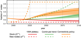
Figure 7 Scenarios for street-network connectivity. We develop 3 scenarios for the connectivity of new nodes, i.e. intersections (dashed lines): (1) 1994 plateau: the fraction of new 4+ degree nodes d4+ plateaus at the 1994 level (the year of peak sprawl); (2) continued trend: d4+ continues to increase at the 1994–2012 rate, until it reaches 0.65; and (3) connectivity policy: d4+ increases rapidly after 2015, to reach 0.65 in 2025. We then calculate the impact of these new nodes on the connectivity of the stock D4+ (solid lines, with envelope). The speed with which new nodes influence the stock depends on the amount of new construction, and the shaded intervals reflect the bounds of the housing projections in figure 8.
Download figure:
Standard image High-resolution image2.2.2. Estimating travel and emissions impacts
While the scenarios are defined in terms of the connectivity of new streets, it is the connectivity of the entire stock of streets that affects travel behavior. Thus, the impact of the trends in d4+ will depend on how they affect the fraction of 4+ degree nodes in the stock, denoted D4+, which in turn depends on the assumed rate of urban growth.
We use growth in the housing stock to estimate the growth of the street-network stock. We assume that the growth rate of nodes, γN, is linearly proportional to the annual growth rate γH of the housing stock, so that γN = νγH, where ν (dimensionless) denotes the nodes-to-housing growth ratio. We derive γH from the housing growth forecasts in Zeng et al [37], with the starting value adjusted to match the 2013 retrospective revision from the US Census Bureau. Alternative projections for housing growth provide similar estimates (figure 8).
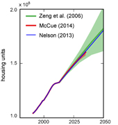
Figure 8 Three projections of future housing unit growth in the USA. All three series project similar trends. Shaded envelopes for Zeng et al [37] and McCue [18] represent the published uncertainty bounds, which reflect different scenarios for population growth and (in the case of Zeng et al [37]) household formation, rather than statistical uncertainty. Nelson [22] provides only central estimates. Projections are aligned with the latest historical data from the Census Bureau.
Download figure:
Standard image High-resolution imageWe extrapolate the trends beyond 2050 by assuming a constant rate of new units added (∼1.25 million year−1), based on the 2040–2050 average. The same procedure is used to separately extrapolate each bound of the uncertainty envelope. These data points give us a central estimate for γH of 1.1% in 2014, declining to 0.5% by 2100. Importantly, the housing growth figures refer to net new units rather than total new construction; the latter is ∼42% greater than the former according to [22].
We estimate the nodes-to-housing growth ratio ν at ∼1.4 using our historical street-network data, which we describe in full in [1]. A value of ν of greater than one indicates that the street network grows at a faster rate than the net housing stock. This could be partly driven by more rapid growth in non-residential development, and partly by the replacement of housing units in a different geographic location (e.g. abandoned housing in Detroit or New Orleans being replaced by units in Phoenix). The relationship between ν and sprawl is unclear a priori. Less sprawl might lead to a lower value of ν if new housing units take the form of tall apartment buildings, or a higher value of ν if less sprawl is accompanied by smaller blocks. Therefore, we assume that ν is constant rather than a function of the level of sprawl.
Given estimates for γH and ν, we proceed to estimate the impact of trends in d4+, the fraction of 4+ nodes in new construction, on the fraction D4+ in the stock. The growth rate in the stock N of nodes, i.e. the number of intersections, evolves as:

The connectivity of the stock (shown in figure 7, solid lines) then evolves as:
Finally, we use our projections of D4+ to estimate changes in vehicle travel, energy use and CO2 emissions, using two estimates for the elasticity of vehicle travel with respect to D4+. Assuming that fleet fuel efficiency and fuel carbon content are not affected by D4+, the elasticity of vehicle travel will be identical to those for household vehicle energy consumption and CO2 emissions. The analysis in section 2 provides the first elasticity estimate, −0.15. The second estimate, −0.12, is taken from the meta-analysis in Ewing and Cervero [10]. Based on an elasticity  , the one-year fractional change in vehicle distance and hence emissions δE is as follows:
As with any application of elasticities, equation (5) is only valid for small changes in D4+. Under the assumption of constant elasticity (see section 5.2), the accumulated changes in emissions from the 2015 baseline can be calculated as:
The two elasticity estimates combined with the three housing growth estimates (the central projection and bounds in figure 8) generate six values for each scenario. Our central estimate uses the central estimate for housing growth combined with our preferred elasticity (−0.15). The shaded envelope represents the highest and lowest of the six values.
We assume that the level of sprawl does not affect the fuel efficiency of vehicles nor the carbon content of fuels, and thus δE is the same as the fractional change in private vehicle travel. This assumption is also used in [32]. Because we ultimately compare fractional changes across scenarios, this does not imply constant fuel economy or carbon content over the 2015–2100 period, but rather that any changes over time are identical across our three scenarios. Vehicles are likely to become more efficient and shift to electricity and other fuels over this time frame, and autonomous vehicles may become widespread. These changes will affect the absolute emissions impacts, but provided that the factors are independent, we provide valid estimates of the proportional emissions impacts of trends in street-network sprawl.
3. Results and analysis
In 3.1 below we present the instrumental variables estimate of the elasticity of vehicle ownership, including our first-stage estimates predicting connectivity as the fraction of 4+ degree nodes or their mean degree. Section 3.2 then presents our main results from applying the elasticity for D4+ to future projections of new road construction.
3.1. Elasticity of vehicle ownership
Table 2 shows our first stage estimates, which predict street-network connectivity from topographic steepness. The first row shows that as a block group becomes 10% steeper9, the predicted fraction of 4+ intersections D4+ decreases by 9%, and predicted mean nodal degree  decreases by about 2%. The 'β coef' row shows the same coefficients expressed in standardized form. These show that a one standard deviation in our steepness variable accounts for between 25% and 30% of a standard deviation in our measures of connectivity. Using these estimates, the component of variation in D4+ predicted by topography is used in the second-stage regression to identify the effect on vehicle ownership.
Our findings for the unitless elasticities β0 are shown in table 3. In odd-numbered columns, we show ordinary least squares estimates using the overall variation in street network connectivity to account for differences in transportation outcomes. Even-numbered columns present our favored IV estimates which focus on the exogenously-influenced component of the street‐network connectivity.
Table 3. Estimates of road network connectivity elasticity of vehicle ownership. Coefficients and (in parentheses) their standard errors are calculated using 2013 data for all US urban block groups with >50 intersections, and outside of Washington, DC. State or county fixed effects are included as indicated. Data from Washington, DC are dropped in order to be able to cluster standard errors at the county level. Odd-numbered columns are from OLS models, while even-numbered columns are IV estimates, in which only the component of road connectivity accounted for by terrain topography is used to explain variation in transportation outcomes. In order to estimate elasticities, the log of the independent and dependent variables are used in a linear model. The boxed value of −.15 is the value referenced in our later projections.
| log (vehicles/HH) | ||||||||
|---|---|---|---|---|---|---|---|---|
| OLS | IV | OLS | IV | OLS | IV | OLS | IV | |
| (1) | (2) | (3) | (4) | (5) | (6) | (7) | (8) | |
| log (degree) | −.72† | −.72† | −.70† | −1.03† | ||||
| (.016) | (.056) | (.017) | (.048) | |||||
| log (fourway) | −.12† | −.15† | −.12† | −.21† | ||||
| (.003) | (.012) | (.003) | (.010) | |||||
| Instrumented (terrain) | Y | Y | Y | Y | ||||
| f.e./demean | state | state | county | county | state | state | county | county |
| Nclusters | 2 371 | 2 371 | 2 371 | 2 371 | 2 371 | 2 371 | 2 371 | 2 371 |
| Weak ID F | 710 | 739 | 849 | 547 | ||||
| F | 75.5 | 161 | 1662 | 456 | 72.5 | 168 | 1696 | 458 |
| R2(adj) | .198 | .129 | .122 | .040 | .210 | .149 | .131 | .101 |
| obs. | 63 360 | 63 360 | 63 360 | 63 360 | 63 480 | 63 480 | 63 480 | 63 480 |
In accordance with the strength of the relationships shown in table 2, our first-stage estimates pass standard tests of weak- and under-identification of the instruments. These estimates are characterized by the following: high statistical confidence in all cases; general consistency across OLS and IV estimates; somewhat larger elasticities from IV models as compared with OLS; and a close agreement of the D4+-elasticity of vehicles per household with the meta-analysis elasticity reported by Ewing and Cervero [10]. We use the elasticity of –0.15 highlighted in a box in table 3 in order to make projections about the future growth of vehicle travel and emissions. This value means, for instance, that on average a fractional change of +10% in the value of D4+ leads to a fractional decrease of 1.5% in the number of vehicles owned by households. Of course, there are many other determinants of car ownership beyond urban form, not least fuel prices, and income, age and other socioeconomic factors. Our aim here is not to comprehensively explain variation in car ownership, but rather to isolate the causal impact of a change in street-network sprawl.
In section 5.2 of the supplementary information, we detail some further checks on these results, and we find them robust to inclusion of other controls and to the allowance for spatial spillovers and spatially correlated errors (estimated using [6]). We also find similar elasticities across a range of values of D4+—i.e. for neighbourhoods with both relatively low and relatively high connectivity.
3.2. Emissions scenarios
We now use our elasticity estimate from section 3.1 to project the emissions impacts of scenarios for street-network connectivity, in line with the method discussed in section 2.2. We report projected cumulative changes compared with the 2015 baseline year. The impact of declining street-network sprawl on vehicle travel and emissions takes time to accrue, given that new construction influences the stock of streets only incrementally. However, by 2050, a continued trend (Scenario 2) implies a ∼3.2% reduction (range of 1.6%–4.2%) against the 2015 baseline in household vehicle travel and emissions compared to Scenario 1, under which sprawl plateaus at its 1994 peak (figure 9). A policy scenario with immediate action to promote a gridded street network (Scenario 3) yields an even larger reduction of ∼5.6% (3.2%–6.6%) compared to Scenario 2, and ∼8.8% (4.8%–10.7%) compared to Scenario 1. The ranges given in parentheses reflect the uncertainty envelopes shown in figure 9, which encapsulate different assumptions about growth in the street network and the elasticity of vehicle travel with respect to street-network sprawl, as discussed in 2.2.210.

Figure 9 GHG implications of a continued decline in sprawl. We use the three scenarios shown in figure 7 to estimate the impact on vehicle distance traveled and GHG emissions from light-duty vehicles.
Download figure:
Standard image High-resolution image
Beyond 2050, the uncertainty envelope widens considerably due to compounded uncertainties in the growth of the housing stock. Added to this is uncertainty from non-quantified factors, not least a potential shift to automated vehicles [15]. Figure 9 plots the projections through 2100, primarily to illustrate how differences between the scenarios continue to widen after 2050 as post-2012 nodes account for an increasing proportion of the stock over time. By 2100, the continued trend of Scenario 2 produces a ∼9.5% reduction in vehicle travel compared to Scenario 1, with a further ∼4.4% reduction from the connectivity policy of Scenario 3.
Towards the end of the century, Scenarios 2 and 3 begin to converge as d4+ hits its assumed ceiling of 0.65 in both scenarios in 2094. The 'wedge' between the two scenarios indicates the emission savings from immediate concerted policy action, rather than waiting for the trends to run their course.
In the United States, light-duty vehicles are projected to account for ∼744 Mt CO2 or ∼13% of energy-related CO2 emissions in 2040 ([7], EIA reference case; projections do not extend beyond 2040). Assuming that 2050 baseline emissions are the same as 2040, our results suggest that on current trends, CO2 emissions in 2050 would be ∼24 Mt CO2 year−1 lower than Scenario 1, under which street-network sprawl continues unabated. Under the connectivity policy (Scenario 3), they would be ∼65 Mt CO2 year−1 lower than Scenario 1. We do not account for other influences on vehicle travel such as population growth, demographic changes, fuel prices and incomes, and so the scenarios should be interpreted relative to each other rather than in absolute terms. Our scenarios are counterfactuals, rather than a comprehensive integratated assessment exercise.
Our estimates are likely to be at the lower end of probable impacts of street-network sprawl on vehicle travel and CO2 for several reasons. First, we do not account for non-transportation emissions savings. Dimensions of urban form that are correlated with street-network sprawl, such as density, reduce energy and materials consumption in other sectors—for example, because of smaller housing units and a shift towards shared commercial provision of services, from car ownership to fitness centers11. Second, assumptions on the rate of growth of the stock of nodes determine how quickly changes in the connectivity of new nodes affect the connectivity of the stock; our assumptions of ∼0.5%–1.1% annual growth are based on housing market projections, but are below the historic growth rate of ∼1.6% over the 1994–2012 period. Third, we do not consider spillovers through which the characteristics of new streets affect travel by residents on existing streets.
4. Conclusions
Transportation policies to reduce greenhouse gas emissions have traditionally focused on vehicle technology and fuels, such as electric vehicles and fuel economy. However, technology- and fuel-based policies are unlikely to be sufficient to avoid dangerous climate change, and long-term climate targets will likely only be feasible with global implementation of land-use and transportation policies to reduce vehicle travel [28]. Even where the connections between land-use and travel demand are addressed, many technical and policy syntheses, including the transportation chapter of the most recent assessment report from the Intergovernmental Panel on Climate Change [25]12, overlook the mitigation potential of improving street connectivity.
We find that reducing street-network sprawl can make a large contribution to greenhouse gas mitigation, particularly in the medium-to-long term. On current trends alone, we project vehicle travel and emissions to fall by ∼3.2% over the 2015–2050 period, compared to a scenario where sprawl plateaus at its 1994 peak. Concerted policy efforts to increase street connectivity could nearly triple these reductions to ∼8.8% by 2050. Longer-term reductions over the 2050–2100 period are more speculative, but could be more than 50% greater than those achieved by 2050.
Our projected reductions from current trends, even without assuming an accelerated connectivity policy, have an impact of comparable or greater magnitude to the climate policy interventions modeled in various studies. For example, a CO2 price of $30–$60/t from an economy-wide cap-and-trade scheme would reduce vehicle travel in 2030 by ∼1% (although reductions in the energy sector from cap-and-trade would be much greater) [27]. An 'aggressive deployment' of land-use strategies, with at least 64% of new development in 'compact, pedestrian- and bicycle-friendly neighborhoods with high-quality transit' yields a 2.7% reduction in vehicle travel by 2050 [3, p. 42]. A Transportation Research Board/National Research Council special report [32], meanwhile, suggests that doubling density in 25%–75% of new developments would lead to a 1.0%–7.7% vehicle travel reduction by 205013. While policies to reduce travel often yield individually small impacts and can best be viewed in combination, our results suggest that the implementation path may be easier than previously thought.
More concerted policy efforts can accelerate the mitigation benefits. Current trends are likely due to a combination of market preferences and policy initiatives by some local governments. However, state and/or federal government policy could bring about a faster transition to more connected street networks. Some state-level policies have already been implemented, such as the Virginia legislation noted above that strongly discourages cul-de-sacs. Federal policy is also a possibility. Historically, guidelines from the Federal Housing Administration and other agencies contributed to the early 20th Century rise of cul-de-sacs [31]. Thus, federal policy could also work in the opposite direction, and discourage street-network sprawl through mortgage underwriting guidelines, fiscal incentives to states and regional agencies, or market-based policies such as taxes on less-connected street networks. Such taxes would account for the social costs imposed on others, now and in the future, by low-connectivity roads14.
Street-network decisions likely have an additional cost related to future options. The same gridded street network supports, on the one hand, a low-density, single-family housing neighborhood with large lots and, alternatively, contiguous apartment buildings or even skyscrapers. By contrast, low-connectivity street-network sprawl is mostly good for just one specialized option involving low-density, car-oriented living. In the long run, prices, transportation modes, work habits, and consumption patterns may be hard to predict, and are certainly not captured in our projections. In this sense, the ability of urban regions to adapt quickly to new circumstances is ultimately the most valuable asset. Urban landscapes like the municipalities of Los Angeles and Vancouver have the option to transform transit and cycling infrastructure, residential density, and land-use mix rapidly, on account of having a largely gridded road network.
The case of street-network sprawl also highlights the need for a package of mitigation policies that operate over different time scales. Increasing street connectivity will do little to contribute to the immediate emission reductions that are needed to avoid the risks of overshooting an atmospheric CO2 concentration that reduces the risks of dangerous climate change [4, 26]. However, the longer the timescale, the more important it becomes to address the physical form of the built environment. While emission reductions from connectivity policies are substantial by 2050, they become even steeper by 2100 (figure 9). Moreover, the costs of waiting are amplified by the persistence of urban streets. A new car might be on the road for 15 years, and a new coal-fired power station might last several decades, but cul-de-sacs can lock in a high-emissions pathway for a century or more.
Acknowledgments
We thank Alain Plante for his patience and expertise in support of our computation server. This work was supported by the Social Sciences and Humanities Research Council of Canada, grant 435-2016-0531.
Footnotes
- 4
The dataset is based on the US Census Bureau TIGER/Line street network, and makes adjustments such as merging adjacent nodes that are functionally part of the same intersection. For full details, see the supporting information in Barrington-Leigh and Millard-Ball [1].
- 5
On average, households in states with higher-connectivity roads are also less likely to commute alone by car; see the supplementary information.
- 6
Although we do not make use of state-level estimates in what follows, we also tested the state-level findings shown in table 2 for sensitivity to outliers. Using the robust regression model in Stata, in which influential observations are progressively down-weighted, did not change the point estimates.
- 7
Ideally, for the instrumental variables interpretation to hold, the influence of terrain on road network properties would occur only through the extra difficulty of conforming a gridded or highly connected network on uneven or steep ground. By contrast, indirect causal effects such as the selection of a different demographic, with different preferences for housing style or transport modes, towards steeper terrain would invalidate this approach. For our instrumented estimates, we assume that these alternate pathways are weak. We apply both uninstrumented (ordinary least squares) models as well as instrumented (two stage least squares) models in order to compare estimates.
- 8
We measure connectivity as the fraction of 4+ degree nodes, rather than nodal degree, in order to match estimates of elasticities in the literature.
- 9
Recall that we measure steepness as the fraction of ∼10 m × ∼10 m grid cells within a block group that are steeper than 10°. Thus, a 10% increase in steepness means that an additional 10% of the land area exceeds this 10° threshold.
- 10
Note that these ranges cannot be computed directly from figure 10. For example, the upper bound of the envelope in Scenario 1 does not necessarily reflect the same combination of street-network growth and elasticity assumptions as the upper bound of Scenario 3.
- 11
On a per capita basis, low-density development is more than twice as intensive in both energy use and GHG emissions as high-density development in the urban core, taking into account infrastructure and building materials and operations, and public and private transportation [23].
- 12
Chapter 8, Transport, of the IPCC report mentions street connectivity only as a brief aside, although the topic is covered in more detail in the same report in chapter 12, Human Settlements, Infrastructure, and Spatial Planning.
- 13
The report notes that the higher-end estimates would be 'challenging,' and that the committee was split over the feasibility of achieving such a change in urban densities. On the other hand, [11] suggests a much higher impact than the TRB/NRC study.
- 14
We suggest that such a market-based policy be known as the 'cul-de-tax.'