
Abstract
Assessing the performance of climate models in surface air temperature (SAT) simulation and projection have received increasing attention during the recent decades. This paper assesses the performance of the Coupled Model Intercomparison Project phase 5 (CMIP5) in simulating intra-annual, annual and decadal temperature over Northern Eurasia from 1901 to 2005. We evaluate the skill of different multi-model ensemble techniques and use the best technique to project the future SAT changes under different emission scenarios. The results show that most of the general circulation models (GCMs) overestimate the annual mean SAT in Northern Eurasia and the difference between the observation and the simulations primarily comes from the winter season. Most of the GCMs can approximately capture the decadal SAT trend; however, the accuracy of annual SAT simulation is relatively low. The correlation coefficient R between each GCM simulation and the annual observation is in the range of 0.20 to 0.56. The Taylor diagram shows that the ensemble results generated by the simple model averaging (SMA), reliability ensemble averaging (REA) and Bayesian model averaging (BMA) methods are superior to any single GCM output; and the decadal SAT change generated by SMA, REA and BMA are almost identical during 1901–2005. Heuristically, the uncertainty of BMA simulation is the smallest among the three multi-model ensemble simulations. The future SAT projection generated by the BMA shows that the SAT in Northern Eurasia will increase in the 21st century by around 1.03 °C/100 yr, 3.11 °C/100 yr and 7.14 °C/100 yr under the RCP 2.6, RCP 4.5 and RCP 8.5 scenarios, respectively; and the warming accelerates with the increasing latitude. In addition, the spring season contributes most to the decadal warming occurring under the RCP 2.6 and RCP 4.5 scenarios, while the winter season contributes most to the decadal warming occurring under the RCP 8.5 scenario. Generally, the uncertainty of the SAT projections increases with time in the 21st century.
Export citation and abstract BibTeX RIS

Content from this work may be used under the terms of the Creative Commons Attribution 3.0 licence. Any further distribution of this work must maintain attribution to the author(s) and the title of the work, journal citation and DOI.
Global atmospheric concentrations of greenhouse gases have significantly increased since the pre-industrial era. The increasing concentration of greenhouse gases is an important reason for global warming from the last century with high confidence (Yang et al 2011). During the 20th century, the average surface air temperature (SAT) of the Northern Hemisphere has risen approximately 1 °C (IPCC 2007, Polyakov et al 2012). As outlined in the fourth assessment report (AR4) of the Intergovernmental Panel on Climate Change (IPCC), even if greenhouse gases are stabilized at the level in 2000, the average global temperature will increase approximately 0.1 °C every decade (IPCC 2007).
Increases in the temperature may have serious influence on the natural and social aspects, such as water availability (Piao et al 2007, Gosling and Arnell 2011, Miao et al 2009, Sheffield et al 2012), food security (Tubiello et al 2007, Lobell et al 2008, Piao et al 2010), ecological environment (Allen et al 2010, Miao et al 2010, Tabari et al 2013, Yang et al 2013, Yang et al 2014), species biodiversity (Wake and Vredenbury 2008, Nowak 2010), and human health (Robine et al 2008, Gosling et al 2009) etc These influences have urged the scientific and social communities to improve understanding of the causes and consequences of global warming (Sun et al 2014). Moreover, policymakers need the latest information on the likely future impacts of climate change to reconcile human society with natural systems.
Northern Eurasia accounts for about 20% of the Earth's land surface and 60% of the terrestrial land cover north of  (Groisman et al 2009). It contains vast areas of wetlands, especially peatland, which contains a large amount of organic carbon and is often underlain by continuous and discontinuous permafrost (Zhu et al 2011). Compared with low latitude regions, Northern Eurasia, especially its northern areas, has been under more dramatic environmental changes in the 20th century, including increasing temperatures, melting permafrost, changing precipitation and prolonged growing seasons (Romanovsky et al 2007, IPCC 2007). According to observation, Northern Eurasia is the region with the largest and the steadiest SAT increases, and warming became most pronounced during the second half of the 20th century (Groisman et al 2007). During the period of widespread instrumental observations in Northern Eurasia (since 1881), the annual surface air temperature has increased 1.5 °C (while 3 °C in the winter season) (Groisman and Soja 2009). There is a statistically significant increase in the number of thaw days over Northern Eurasia (McBean et al 2005), which is primarily due to the reduction of days with frost, ice and remnant snow on the ground rather than due to the snow cover retreat (Groisman et al 2006). However, there is an interesting phenomenon in Northern Eurasia found by Bulygina et al (2011) that most areas of Northern Eurasia have experienced an increase in both winter average and maximum snow depths in recent decades, which is against the background of global temperature rise and sea ice reduction in the northern hemisphere.
Climate projections and their associated applications have become an important topic during recent decades. Several research teams around the world develop models to simulate the current climate and its future evolution under different greenhouse gas and aerosol scenarios (Buser et al 2009). Global coupled Atmospheric-Ocean General Circulation Models (coupled GCMs) are the modeling tools traditionally used in theoretical investigations of climatic change mechanisms (Covey et al 2003). By using GCMs, we can not only simulate the present-day and project future climatic changes under different scenarios but also separate natural climate variability from anthropogenic effects.
The GCMs simulations for the fifth assessment report (AR5) of the IPCC have recently become available (Taylor et al 2012). Comparing to the IPCC AR4, the GCMs in AR5 include a more diverse set of model types (i.e., climate/Earth system models with more interactive components such as atmospheric chemistry, aerosols, dynamic vegetation, ice sheets and carbon cycle) (Liu et al 2013). A number of improvements in the physics, numerical algorithms and configurations are implemented in the IPCC AR5 models with a new set of scenarios called representative concentration pathways (RCPs) used in the AR5 simulations (Moss et al 2010). The RCPs span a large range of stabilization, mitigation and non-mitigation pathways. Consequently, the range of the temperature estimates is larger than that of the scenarios in the AR4, which only covers non-mitigation scenarios (Rogelj et al 2012). It is expected that some of the scientific questions that occur during the preparation of the IPCC AR4 will be addressed in the AR5 (Taylor et al 2012).
The climate change in Northern Eurasia is a topic of great interest, and the amount of research associated with the GCMs is developed. However, previous analyses are primarily focused on the early experiments of the IPCC. An evaluation and application of the updated generation of the AR5 GCMs in Northern Eurasia is missing. In this study, we focus on the state-of-the-art models that have been made publically available through the Coupled Model Intercomparison Project phase 5 (CMIP5). This study is aimed at answering the following questions: 1) how well do the AR5 GCMs reproduce the historical SAT patterns; 2) which type of multi-model ensemble techniques can provide the best skill to improve the simulation performance; and 3) what changes in climate means may be expected in the future. Our results potentially provide inputs for climate change impact assessments that explore the probability of climate-related threats in Northern Eurasia.
1. Data and methods
1.1. Data
Observations of monthly SAT over Northern Eurasia are obtained from the Climate Research Unit data (CRU TS 3.1) (Mitchell and Jones 2005, Harris et al 2013) (available at http://badc.nerc.ac.uk/data/cru/). The horizontal resolution of the dataset is 0.5° × 0.5°, and the time period in this research is from 1901 to 2005.
24 GCMs outputs obtained from the CMIP5 data archive (http://cmip-pcmdi.llnl.gov/cmip5/index.html) are listed in table 1. The monthly data includes the historical (1901–2005) and the future (2006–2099) periods. Here we focus on the SAT projection under three scenarios (i.e., RCP 2.6, RCP 4.5 and RCP 8.5). The three RCPs represent 'low' (RCP 2.6), 'medium' (RCP 4.5) and 'high' (RCP 8.5) scenarios featured by the radiative forcings of 2.6, 4.5 and 8.5 W m−2 by 2100, respectively. The CO2-equivalent concentrations in the year 2100 for RCP 2.6, RCP 4.5 and RCP 8.5 are 421 ppm, 538 ppm and 936 ppm, respectively (Meinshausen et al 2011). For comparison purpose, all GCM outputs are regridded to the same resolution as that of the observed data (0.5° × 0.5° grid).
Table 1. List of the global climate models in IPCC-AR5.
| GCM | Model | Resolution | Source |
|---|---|---|---|
| 1 | BCC-CSM 1.1 | 64 × 128 | Beijing Climate Center, China Meteorological Administration, China |
| 2 | BCC-CSM1.1(m) | 160 × 320 | |
| 3 | BNU-ESM | 64 × 128 | Beijing Normal  , China , China |
| 4 | CanESM2 | 64 × 128 | Canadian Centre for Climate Modelling and Analysis, Canada |
| 5 | CCSM4 | 192 × 288 | National Center for Atmospheric Research (NCAR), USA |
| 6 | CNRM-CM5 | 128 × 256 | Centre National de Recherches Meteorologiques, France |
| 7 | CSIRO-Mk3.6.0 | 96 × 192 | Australian Commonwealth Scientific and Industrial Research Organisation |
| 8 | FGOALS-g2 | 108 × 128 | Institute of Atmospheric Physics, Chinese Academy of Sciences, China |
| 9 | FIO-ESM | 64 × 128 | The First Institute of Oceanography, SOA, China |
| 10 | GFDL-CM3 | 90 × 144 | Geophysical Fluid Dynamics  , USA , USA |
| 11 | GFDL-ESM2G | 90 × 144 | |
| 12 | GISS-E2-H | 90 × 144 | Goddard Institute for Space Studies (NASA), USA |
| 13 | GISS-E2-R | 90 × 144 | |
| 14 | HadGEM2-ES | 145 × 192 | Met Office Hadley  , UK , UK |
| 15 | IPSL-CM5A-LR | 96 × 96 | Institut Pierre-Simon Laplace, France |
| 16 | IPSL-CM5A-MR | 143 × 144 | |
| 17 | MIROC5 | 128 × 256 | Atmosphere and Ocean Research Institute, University of Tokyo, Japan |
| 18 | MIROC-ESM | 64 × 128 | Japan Agency for Marine-Earth Science and Technology, Atmosphere and Ocean Research Institute (The University of Tokyo), Japan |
| 19 | MIROC-ESM-CHEM | 64 × 128 | |
| 20 | MPI-ESM-LR | 96 × 192 | Max Planck Institute for Meteorology (MPI-M), Germany |
| 21 | MPI-ESM-MR | 96 × 192 | |
| 22 | MRI-CGCM3 | 160 × 320 | Meteorological Research Institute, Japan |
| 23 | NorESM1-M | 96 × 144 | Norwegian Climate Centre, Norway |
| 24 | NorESM-ME | 96 × 144 |
1.2. The methodology of multi-model ensemble averaging
Because single models are overconfident (Weigel et al 2008) and multi-model ensembles contain information from all participating models (Pincus et al 2008), it is generally believed that multi-model ensembles are superior to single models (IPCC 2001, Duan and Phillips 2010, Miao et al 2013). In this study, three types of popular ensemble methods are used. They are simple model averaging (SMA), reliability ensemble averaging (REA) and Bayesian model averaging (BMA) techniques.
SMA is the simplest multi-model ensemble technique. Each model has the same weight (wk = 1/K, where K is the number of models) in the multi-model forecast. When using the SMA, any knowledge about the performance of the model is neglected (Casanova and Ahrens 2009).
The REA is a weighted average of ensemble members method based on the 'reliability' of each model (Giorgi and Mearns 2002). The reliability factor of the kth model (Rk ) takes into account of the ability of each ensemble member to simulate the observed climate (RB ) and its degree of convergence in the projected climate change with respect to the other models in the ensemble (RD ).

where RB
is a factor that is inverse proportional to the absolute bias (B) in simulating the present-day variable and RD
is a factor that measures the model reliability in terms of the distance (D) of the change calculated by a given model from the REA average change. The parameters m and n are the weights of the model performance criterion (RB
) and the model convergence criterion (RD
), respectively, which are typically equal to 1. The parameter  in equation (1) is the natural variability of the climatic variable. More details of the REA process are provided in Giorgi and Mearns (2002) and Mote and Salathé (2010).
The BMA generates a probability density function (PDF), which is a weighted average of the PDFs centered on the forecasts. The BMA weights reflect the relative contributions of the component models to the predictive skill over a training sample. The combined forecast PDF of a variable y is:

where  is the forecast pdf based on the model Mk
alone, estimated from the training period of observations yT; and K is the number of models combined.
is the forecast pdf based on the model Mk
alone, estimated from the training period of observations yT; and K is the number of models combined.  is the posterior probability of the model Mk
corrected using the training data. This term is computed based on Bayes' theory:
is the posterior probability of the model Mk
corrected using the training data. This term is computed based on Bayes' theory:

The BMA weights are estimated using the maximum likelihood (Raftery et al 2005). To estimate given parameters, the likelihood function is the probability of the training data and is viewed as a function of the parameters (Yang et al 2011). The weights are chosen to maximize this function (i.e., the parameter values for which the observation data are most likely to have been observed). The algorithm used to calculate the BMA weights and variance is called the expectation maximization (EM) algorithm (Dempster et al 1977). More details of the BMA process are provided in Raftery (2005) and Duan and Phillips (2010).
1.3. Evaluation process
For GCM performance assessment, the bias between observation and model simulations is compared. The SAT change during the historical period (1901–2005) and the projected future scenarios (2006–2099) are analyzed.
In order to evaluate the ensemble performance, the Taylor diagram technique is used. The Taylor diagram is quantified in terms of the correlation (R), the centered root-mean-square-error (RMSE) and the amplitude of the standard deviations (Std). The diagram provides a way of graphically summarizing how closely a pattern matches observations (Taylor 2001). Moreover, the uncertainty of the different multi-model ensembles is also compared. Here, we calculate the standard deviation of the changes, δ, defined by

where (wk ) is the weight of kth model generated by different multi-model ensemble techniques, Tk is the kth model output and En is the ensemble. The upper and lower uncertainty limits are thus defined as:


If the changes are distributed as a Gaussian PDF, the ±δ range implies a 68.3% confidence interval.
1.4. Temperature projection
It is generally accepted that the agreement between models and observations currently is the only way to assign confidence into the quality of a model (Errasti 2011), and the better a model performance in reproducing present-day climate, the higher the reliability of the climate change simulation (Giorgi and Mearns 2002, Coquard et al 2004). Each GCM's weight can be obtained from the ensemble process during the period of 1901–2005. Applying with these weights, multi-model ensemble projections in temperature over the 21st century scenarios can be generated.
2. Results
2.1. Model bias and warming trend
Figure 1 shows the bias in 24 CMIP5 climate models by comparing the observed and simulated data of the 105 year annual and seasonal mean temperatures. Most of the GCMs give reasonably accurate predictions of the mean temperature. Among the 24 GCMs, nine models underestimate the annual mean temperature, while the others overestimate. The maximum bias for SAT simulation comes from the FGOALS-g2 model, with a value of −4.31 °C. The BCC-CSM 1.1 and GISS-E2-R models perform the best, with a minimum bias of 0.10 °C. It should be noted that the 105 year mean of observed temperature is about −4.50 °C. It is also found that models with higher resolution do not always perform better than those with lower resolutions (such as the FGOALS-g2 model). For the seasonal SAT simulation, model biases in March–April–May (MAM) and June–July–August (JJA) are relatively small, while the bias in December–January–February (DJF) is high. Compared with the BCC-CSM 1.1 model, the GISS-E2-R model has the smaller bias in the seasonal SAT simulation.
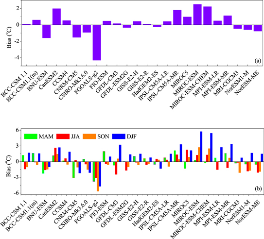
Figure 1. (a) Annual and (b) seasonal bias of different AR5 GCMs with regard to observed mean temperature in Northern Eurasia during 1901–2005.
Download figure:
Standard image High-resolution imageThe SAT observation has increased at a rate of about 1.1 °C/100 yrs during 1901–2005 (figure 2). Among the 24 GCMs, 12 models overestimate the warming trend, and the others overestimate. However, the warming trend differences between the observation and the overestimating models are generally larger than that from the underestimating model. The simulated warming trends by the IPSL-CM5A-LR and MRI-CGCM3 models are closest to the observations, and the maximum warming trend (approximately 2.76 °C/100 yrs) is simulated by the BNU-ESM model. It is widely recognized that if the worst impacts of climate change are to be avoided then the average rise in the surface temperature of the Earth needs to be less than 2 °C. Hence, we project the time when the global land mean SAT (without Antarctica) reaches a 2 °C increase relative to 2000 under different RCPs, and compare with the corresponding SAT increase over Northern Eurasia at that time (table 2). Under the RCP 2.6 scenario, six GCMs (CanESM2, GFDL-CM3, HadGEM2-ES, MIROC5, MIROC-ESM and MIROC-ESM-CHEM) show the global SAT will rise by 2 °C in this century. And only one GCM model (GISS-E2-R) estimates the global SAT will not increase by 2 °C within this century under RCP 4.5. The projected time by the remaining GCMs is dispersed from 2034 to 2081. All GCMs affirm that the global SAT will rise by 2 °C in this century under the RCP 8.5, and most of the models forecast that the projected time will occur from the 2030s–2050s. Under different scenarios, most of GCMs (except BCC-CSM1.1 (m), CSIRO-Mk3.6.0, GISS-E2-R and MPI-ESM-LR) believe the warming rate over the Northern Eurasia is higher than the global warming average in this century. And some models (such as GFDL-CM3 in RCP 4.5 and MRI-CGCM3 in RCP 8.5) even show the warming in Northern Eurasia is more than twice faster than the global average.
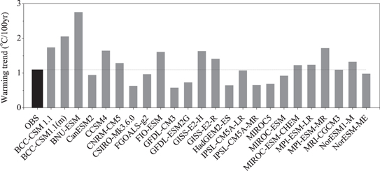
Figure 2. Warming trend for the observations (black bar, left) and each CMIP5 model during 1901–2005.
Download figure:
Standard image High-resolution imageTable 2. The projected time when global land mean SAT increases 2 °C relative to 2000 under different RCPs and the corresponding SAT increases over Northern Eurasia.
| The year global mean SAT increases 2 °C relative to 2000 | Increase in mean SAT over Northern Eurasia when global mean SAT increases 2 °C | |||||
|---|---|---|---|---|---|---|
| Model | RCP26 | RCP45 | RCP85 | RCP26 | RCP45 | RCP85 |
| BCC-CSM 1.1 | × | 2081 | 2052 | × | 2.90 | 2.41 |
| BCC-CSM1.1(m) | × | 2067 | 2049 | × | 1.66 | 1.87 |
| BNU-ESM | × | 2049 | 2039 | × | 3.99 | 2.72 |
| CanESM2 | 2036 | 2036 | 2030 | 2.69 | 2.8 | 2.77 |
| CCSM4 | × | 2063 | 2043 | × | 3.29 | 3.12 |
| CNRM-CM5 | × | 2071 | 2053 | × | 3.29 | 2.68 |
| CSIRO-Mk3.6.0 | × | 2054 | 2045 | × | 1.92 | 1.74 |
| FGOALS-g2 | 2056 | 2039 | × | 3.01 | 2.93 | |
| FIO-ESM | × | 2058 | 2059 | × | 2.27 | 1.81 |
| GFDL-CM3 | 2027 | 2026 | 2025 | 3.61 | 4.5 | 3.09 |
| GFDL-ESM2G | × | 2052 | 2049 | × | 3.38 | 3.06 |
| GISS-E2-H | × | 2059 | 2043 | × | 3.08 | 3.32 |
| GISS-E2-R | × | × | 2054 | × | × | 1.89 |
| HadGEM2-ES | 2024 | 2034 | 2032 | 3.62 | 3.35 | 2.93 |
| IPSL-CM5A-LR | × | 2047 | 2042 | × | 3.55 | 3.11 |
| IPSL-CM5A-MR | × | 2060 | 2046 | × | 2.51 | 2.79 |
| MIROC5 | 2041 | 2043 | 2034 | 2.11 | 2.32 | 2.17 |
| MIROC-ESM | 2045 | 2040 | 2033 | 3.14 | 2.60 | 2.56 |
| MIROC-ESM-CHEM | 2027 | 2027 | 2028 | 3.52 | 3.64 | 3.70 |
| MPI-ESM-LR | × | 2063 | 2042 | × | 1.23 | 1.06 |
| MPI-ESM-MR | × | 2061 | 2043 | × | 3.30 | 2.11 |
| MRI-CGCM3 | × | 2077 | 2045 | × | 3.62 | 4.09 |
| NorESM1-M | × | 2045 | 2043 | × | 2.27 | 2.27 |
| NorESM-ME | × | 2052 | 2047 | × | 3.21 | 2.22 |
Symbol '×' means the rise in global SAT will not reach 2 °C in this century.
2.2. Evaluation of temporal SAT simulation
Figure 3 shows the performance of the annual SAT simulation over the Northern Eurasia. The annual mean SAT observation increases during 1901–2005, and the warming has accelerated since the mid-20th century. Compared with the CMIP3 model, the CMIP5 model improves slightly in the annual SAT simulation, showing as closer to the observation point in the Taylor diagram (figure 3(a)). It is also indicated that most of the GCMs can approximate the trend of SAT, but the accuracy of annual SAT simulation is relatively low. The correlation coefficient R between each GCM simulation and the annual observation ranges from 0.20 to 0.56 (figure 3(a)). The ensemble results show that the ensemble technique can improve the temporal SAT simulation when compared to a single GCM (figure 3(b)). For multi-model ensemble simulation, the performances of the SMA, REA and BMA are similar since their outputs nearly overlap in the Taylor diagram. Comparing the weights generated by BMA and REA techniques, it is found that the model weights are similar but not identical. This is an interesting phenomenon that SMA, REA and BMA generate very similar results, even though the ensemble members receive different weights through the three ensemble techniques.
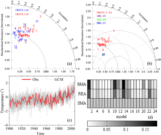
Figure 3. The performance of the annual SAT simulation over Northern Eurasia. (a) Taylor diagram for each model SAT simulation from CMIP5 (red) and CMIP3 (blue, model information see the online supplementary material (stacks.iop.org/ERL/0/000000/mmedia) datasets; (b) comparison between annual SAT simulation from CMIP5 and their ensembles; (c) annual mean SAT anomalies from CMIP5 (relative to the 1970–1999); (d) weights of different ensemble processes.
Download figure:
Standard image High-resolution imageBecause a GCM cannot accurately reflect the actual annual SAT change (figure 3(b)), here we focus on the decadal SAT simulation (figure 4). It shows that GCM can catch the trend of 10-year moving average SAT over Northern Eurasia. Compared with the annual scale, the correlation coefficients between the decadal SAT simulations and observation are increased, being primarily between 0.6 and 0.9; and the ensemble technique can improve the decal SAT simulation further (figure 4(a)). Similar to figure 3(b), the decadal SAT changes simulated by three kinds of ensemble mean methods are almost the same (figure 4(b)). Besides ensemble average, uncertainty is another important skill score. Hence, the uncertainty of the multi-model ensembles during the period of 1901–2005 is also compared. Figure 5 shows the ensemble uncertainty of the simulated results with a 10 year moving average. It is indicated that the uncertainty generated by the BMA is the smallest among the three multi-model ensemble results for simulating the annual and seasonal SAT. In addition, the results show that the uncertainty in DJF is the largest over Northern Eurasia.

Figure 4. The performance of decadal SAT simulation. (a) Taylor diagram for each model and ensemble SAT simulation on decadal scale. (b) Ensemble for decal SAT simulation.
Download figure:
Standard image High-resolution image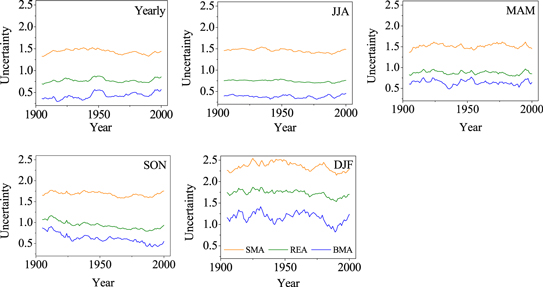
Figure 5. The ensemble uncertainty of annual and seasonal SAT simulated results with a 10-year moving average.
Download figure:
Standard image High-resolution image2.3. Projected SAT change in the 21st century
Considering the smallest uncertainty, the BMA method is applied to project the SAT change in the 21st century under the three future emission scenarios (RCP 2.6, RCP 4.5, RCP 8.5) (figure 6). Only the decadal SAT is projected, due to the poor performance on the annual scale. The BMA simulations show that the SAT of Northern Eurasia will increase remarkably over the 21st century. On average, the SAT over Northern Eurasia will rise by 1.03 °C/100 yr, 3.11 °C/100 yr and 7.14 °C/100 yr for the RCP 2.6, RCP 4.5 and RCP 8.5 scenarios, respectively. Under the RCP 2.6 and RCP 4.5 scenarios, the greatest contribution to the decadal warming is from MAM, while DJF is the largest contributor under the RCP 8.5 scenario. The warming trend slows down or even declines after 2050 under RCP 2.6. For the uncertainty of the SAT projections, it is found that the uncertainty of SAT projections increases with time in the 21st century, and the uncertainty under RCP 8.5 is larger than that under RCP 2.6 and RCP 4.5.
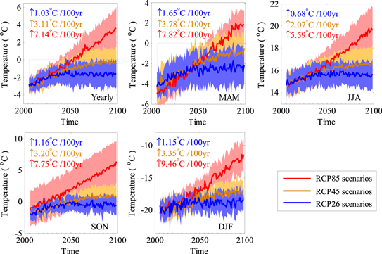
Figure 6. SAT projections over the 21st century using the BMA method. Shown are the evolutions under three emission scenarios derived by applying a 10 yr moving average. Solid lines are the Bayesian multi-model averages of SAT in Northern Eurasia under the scenarios RCP85 (red line), RCP45 (yellow line) and RCP26 (blue line). The color text indicates the average rate of warming under the scenarios RCP85 (red), RCP45 (yellow) and RCP26 (blue). Shading denotes the ±1 standard deviation range of the BMA results with a 10-year moving average.
Download figure:
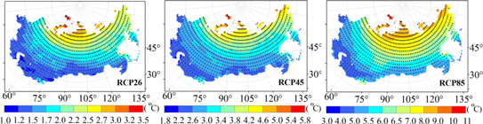
Standard image High-resolution imageFigure 7 shows the projected annual mean SAT change for 2080–2099. The annual mean SAT in the last two decades of 21st century relative to 1986–2005 over Northern Eurasia will increase 1.92 °C, 3.25 °C and 6.40 °C under the RCP 2.6, RCP 4.5 and RCP 8.5 scenarios, respectively. It is found that the warming climate accelerates with increasing latitude. Grids with maximum SAT changes are concentrated in the Svalbard region of Norway under three scenarios, the corresponding changes are 3.61 °C, 5.57 °C and 10.24 °C under the RCP 2.6, RCP 4.5 and RCP 8.5, respectively.
Figure 7. Bayesian model averaging of annual mean SAT change (compared to 1986–2005 base period) for 2080–2099 under different scenarios. Stippling indicates regions where the BMA signal is greater than two standard of internal variability and where 90% of the models agree on the sign of change.
Download figure:
Standard image High-resolution image
3. Discussion and conclusions
This study evaluates and compares the SAT change over Northern Eurasia using the outputs from the GCMs, SMA, REA and BMA, and projects the future SAT trend for different emission scenarios. The major findings of this study are summarized and discussed as follows:
- (1)Most of the GCMs overestimate the annual mean temperature over Northern Eurasia. Similar results are also found in the Arctic (Chylek et al 2011), in the Northern hemisphere (Zhao et al 2013) and globally (Kim et al 2012). The forced and internal variation might contribute the overestimated warming in SAT simulation. It is reported that some CMIP5 models overestimate the responses to the increasing greenhouse gas and other anthropogenic forcing (IPCC 2013). The stratospheric aerosol concentration has increased over the past decade due to the volcanic eruptions, and has cooled global lower-atmosphere temperatures to a statistically significant degree (Santer et al 2014). However, none of the CMIP5 simulations takes this into account (Solomon et al 2011, Santer et al 2014). Moreover, some researchers think the inaccurate way that CMIP5 model handles clouds and water vapor is the main reason for the overestimation. It is found that the CMIP5 model tends to underestimate the cloud cover (Nam et al 2012) and stratospheric water vapor (Fyfe et al 2013a), both of which allow more sun to get in and then to heat up the planet during the simulation. Satellite observations suggest that climate models have ignored the negative feedbacks produced by clouds and water vapor (Christy et al 2010). The missing of these negative feedbacks diminishes the warming effects of carbon dioxide (Fyfe et al 2013a,b). Similarly to the CMIP3 (Miao et al 2013), the models with higher resolution do not always perform better than those with lower resolutions. Generally, the error of annual SAT simulation primarily comes from DJF, while the model biases in MAM and JJA are relatively smaller (figure 1(b), figure 3(b), figure 5). Most of the GCMs can approximate the decadal SAT trend, but the accuracy of annual SAT simulation is relatively low. The correlation coefficients R between each GCM simulation and the annual observations range from 0.20 to 0.56. Hence, direct use of the short-term output from single GCM is not recommended. To model the short-term dynamic series, the effective techniques to improve the regional simulation accuracy should be considered in advance.
- (2)The performances of the multi-model ensembles are superior to that of any single GCM. The Taylor diagram shows that all the multi-models ensemble techniques can improve the skill scores of simulations. The SAT changes in Northern Eurasia generated by SMA, REA and BMA are almost identical during 1901–2005. In general, the approach where model weights are determined by the model skill performs better than the method of equally weighing all models (e.g., Yun et al 2003, Tebaldi and Knutti 2007, Räisänen and Ylhäisi 2012). But some researches also obtained similar ensemble results calculated by different methods. Duan and Phillips (2010) analyze the global annual mean continental temperature and precipitation during 1980–1999, and find the results of the SMA and BMA are almost the same. This finding partially reflects the so-called 'equifinality' in which different combinations of model weights produce the same fit to the observation. In fact, the advantages of the uneven weighting ensemble method are mainly exhibited in narrowing the uncertainty (Giorgi and Mearns 2002, Duan and Phillips 2010, Hawkins and Sutton 2011). Comparing the annual and seasonal SAT uncertainties in the outputs of REA and SMA, the uncertainty generated by BMA is the smallest. Unequal weighting ensemble techniques contain the information from all participating models and embrace distinctly different physical parameterizations (Pincus et al 2008). Different model weight is also assigned according to its performance. Consequently, the unequal weight ensemble techniques moderate the uncertainties arising from different parameterizations and dynamical cores in the different GCMs (Zanis et al 2009).
- (3)The SAT projections over Northern Eurasia show that SAT will increase in the 21st century by 1.03 °C/100 yr, 3.11 °C/100 yr and 7.14 °C/100 yr under the RCP 2.6, RCP 4.5 and RCP 8.5 scenarios, respectively. The warming accelerates with increasing latitude. All the maximum warming under the three scenarios is concentrated in the Svalbard region. Under the RCP 2.6 and RCP 4.5 scenarios, the greatest contribution to the decadal warming comes from MAM, and under the RCP 8.5 scenario, DJF becomes the greatest contributor. Compared with RCP 4.5 and RCP 8.5, the warming trend slows down or even starts declining after the 2050s under RCP 2.6. It is primarily because the RCP 2.6 scenario is designed to limit the increase of global mean temperature to 2 °C (van Vuuren et al 2011), and it has a peak in the radiative forcing at approximately 3 W m−2 (approximately 400 ppm CO2) before 2100 and then declines to 2.6 W m−2 by the end of the 21st century (approximately 330 ppm CO2) (Sillmann et al 2013). In addition, it is found that the uncertainty of the SAT projection outputs simulated by the BMA in the 21st century increases with time. The uncertainty change can be explained by its composition. The uncertainty in the SAT projection arises from three distinct sources: the internal variability of the climate system, the model uncertainty and the scenario uncertainty (Hawkins and Sutton 2009). In CMIP5, internal variability is roughly constant through time, and the other uncertainties grow with time, but at different rates (IPCC 2013). For scenario uncertainty, the spread between RCP scenarios is the dominant source of uncertainty by the end of the century (Hawkins and Sutton 2011). Overall, the uncertainty concluded using CMIP5 is not much changed from using CMIP3 (Knutti and Sedlacek 2013). Considering the mitigation and controllability of greenhouse gas, if we assume that the atmospheric concentrations of greenhouse gases decline quite rapidly under all RCPs in the next few decades, the scenario uncertainty may be smaller than that in the current projection. Not surprisingly, we are supposed to pay more attention to the internal variability and inter-model uncertainty in the near future.
GCM serves as a primary tool for studying and understanding climate change. In response to the SAT projections under different scenarios; it is important to make different adaptation and mitigation strategies in Northern Eurasia.
Acknowledgements
The authors appreciate the valuable comments of Professor Pavel Ya Groisman and Dr Linyin Chen. Funding for this research was provided by the National Natural Science Foundation of China (no. 41001153), the National Key Basic Special Foundation Project of China (no. 2010CB951604), Beijing Higher Education Young Elite Teacher Project, and the State Key Laboratory of Earth Surface Processes and Resource Ecology. We are grateful to the Program for Climate Model Diagnosis and Intercomparison (PCMDI) for collecting and archiving the model data and to the Climate Research Unit (CRU) for collecting and archiving the observed climate data.