
Abstract
Regional scale water management analysis increasingly relies on integrated modeling tools. Much recent work has focused on groundwater–surface water interactions and feedbacks. However, to our knowledge, no study has explicitly considered impacts of management operations on the temporal dynamics of the natural system. Here, we simulate twenty years of hourly moisture dependent, groundwater-fed irrigation using a three-dimensional, fully integrated, hydrologic model (ParFlow-CLM). Results highlight interconnections between irrigation demand, groundwater oscillation frequency and latent heat flux variability not previously demonstrated. Additionally, the three-dimensional model used allows for novel consideration of spatial patterns in temporal dynamics. Latent heat flux and water table depth both display spatial organization in temporal scaling, an important finding given the spatial homogeneity and weak scaling observed in atmospheric forcings. Pumping and irrigation amplify high frequency (sub-annual) variability while attenuating low frequency (inter-annual) variability. Irrigation also intensifies scaling within irrigated areas, essentially increasing temporal memory in both the surface and the subsurface. These findings demonstrate management impacts that extend beyond traditional water balance considerations to the fundamental behavior of the system itself. This is an important step to better understanding groundwater's role as a buffer for natural variability and the impact that water management has on this capacity.
Export citation and abstract BibTeX RIS

Content from this work may be used under the terms of the Creative Commons Attribution 3.0 licence. Any further distribution of this work must maintain attribution to the author(s) and the title of the work, journal citation and DOI.
1. Introduction
Watersheds are complex, heterogeneous, systems governed by nonlinear relationships that respond to non-stationary atmospheric forcings across a broad range of time scales. Since Hurst (1951) first identified the presence of long-term scaling in hydrologic time series in 1951, temporal scaling behavior has been demonstrated for an array of hydrologic variables. For example, temporal self-organization (i.e. variance that scales with period of oscillation) has been observed in time series of runoff (Kirchner et al 2000, Pandey et al 1998, Sauquet et al 2008, Schilling and Zhang 2012, Tessier et al 1996, Young and Jettmar 1976, Zhang and Schilling 2005), chemical constituents (Cardenas 2008, Duffy and Gelhar 1985, 1986, Koirala et al 2011), soil moisture (Amenu and Kumar 2005, D'Odorico and Rodriguez-Iturbe 2000, Katul et al 2007), evapotranspiration (D'Odorico and Rodriguez-Iturbe 2000, Katul et al 2007) and groundwater levels (Li and Zhang 2007, Little and Bloomfield 2010, Schilling and Zhang 2012, Zhang and Schilling 2004, 2005, Zhang and Li 2005, 2006), among others.
Analysis of oscillation frequencies in time series shows that watersheds behave as fractal filters, converting white noise signals (like precipitation) into temporally organized outputs (like runoff) where spectral power (i.e. the importance of a given oscillation mode) is inversely proportional to frequency (or directly proportional to the wavelength) (Kirchner et al 2000, Little and Bloomfield 2010, Tessier et al 1996). Duffy and Gelhar (1986) demonstrated that aquifers act as low pass filters letting low frequency variability pass through while attenuating high frequency variability. Recently, spectral techniques have been increasingly applied to groundwater dynamics. Zhang and Schilling (2004) first showed strong temporal scaling of hydraulic head in eight observation wells. Li and Zhang (2007) found groundwater to have greater temporal persistence (i.e. dependence of observations that are farther apart) than runoff. Similarly Amenu and Kumar (2005) showed increasing persistence in soil moisture scaling with depth. Other studies have observed scaling in groundwater head but note break points and scaling exponents that vary by location (Li and Zhang 2007, Little and Bloomfield 2010, Schilling and Zhang 2012, Zhang and Schilling 2004).
To our knowledge no study has explicitly considered the impacts of water management on temporal behavior, even though temporal scaling and long-term persistence (LTP) within hydrologic variables have potentially significant implications for water management. For example, Koutsoyiannis (2003) and Koutsoyiannis and Montanari (2007) argued that, in the presence of LTP, classical statistics do a poor job of capturing system behavior. Similarly, both Douglas et al (2002) and Young and Jettmar (1976) showed that ignoring persistence can skew analysis of recurrence intervals and result in inappropriate reservoir sizing.
Most previous analysis is based on observed time series and is intentionally focused on locations with small anthropogenic influence (e.g. Sauquet et al 2008, Tessier et al 1996). In locations where the available time series are influenced by water management (e.g. Pandey et al 1998), or in studies using tracers associated with agriculture (e.g. Zhang and Schilling 2005), management operations are discussed but are not the focus of analysis. Here, we take a unique approach by focusing specifically on irrigated agriculture. We simulate moisture dependent groundwater-fed irrigation using an integrated three-dimensional hydrologic model capable of resolving groundwater–surface water interactions as well as feedbacks between irrigation demand and groundwater depth.
This study is also unique in its consideration of spatial patterns in temporal organization. Zhang and Schilling (2004) as well as Li and Zhang (2007) identified spatial variation in temporal scaling of groundwater as an area for future research. While this topic has been explored using point data and one-dimensional models (Li and Zhang 2007, Little and Bloomfield 2010, Schilling and Zhang 2012, Zhang and Li 2005), no study has considered scaling behavior spatially using gridded results. Furthermore, previous studies have been limited by relatively short observation periods of about five years (e.g. Little and Bloomfield 2010, Zhang and Schilling 2004). Using the modeling approach we are able to simulate twenty years of hourly data for each scenario.
2. Methods
2.1. Model and simulations
All results are generated using the integrated physical hydrology model ParFlow-CLM. ParFlow solves three-dimensional variably saturated groundwater flow and fully integrated surface water flow. Land surface processes like soil moisture, plant evapotranspiration and sensible heat flux are simulated using the common land model (CLM). The coupled ParFlow-CLM model integrates surface and subsurface processes and is fully mass and energy conservative. Technical details of ParFlow-CLM are provided in Ashby and Falgout (1996), Dai et al (2003), Jones and Woodward (2001), Kollet and Maxwell (2008b), Maxwell (2013), and Maxwell and Miller (2005). Dynamic, moisture dependent, groundwater-fed irrigation is simulated using the water allocation module (WAM) coupled to ParFlow (Condon and Maxwell 2013). Using ParFlow-CLM with WAM we simulate groundwater–surface water interactions as well as direct feedbacks between groundwater pumping, surface irrigation and subsurface water content. Additionally, this modeling approach allows for high temporal resolution of spatially distributed outputs for a large number of hydrologic variables including water table depth, ground temperature, latent heat flux and sensible heat flux. The primary limitations of this integrated modeling approach are the computational cost and extensive input requirements (i.e. gridded subsurface and land cover parameters as well as meteorological forcings). Computational burden can be defrayed with parallel implementation and here we select a domain for which all model inputs are derived from publically available national datasets.
We present two twenty-year simulations of the Little Washita basin located Southwestern Oklahoma, USA. The Little Washita is a moderately sized basin (∼1600 km2) characterized by grasslands, rolling terrain and a semi arid climate. Previous work analyzed groundwater–surface water interactions and residence time scaling in a similar domain using ParFlow-CLM (Ferguson and Maxwell 2010, 2011, 2012, Kollet and Maxwell 2008a,b, Maxwell et al 2007). For this analysis, simulations encompass a 41 by 41 km domain extending 100 m below the surface using ParFlow's terrain following grid (Maxwell 2013). Results are generated at 1 km2 lateral and 2 m vertical resolution for a total of nearly 85 000 grid cells. Heterogeneous physical parameters including land cover (NASA 2001) as well as soil (Miller and White 1998) and subsurface parameters (Gleeson et al 2011) are derived from available datasets in order to generate a realistic domain. Soil conductivity values range from 0.003 to 0.27 m h−1 while values for the deeper subsurface (i.e. below 2 m) are slightly higher from 0.02 to 0.68 m h−1 (see figure S1, available at stacks.iop.org/ERL/9/034009/mmedia).
Two scenarios one with irrigation (Irrigation) and one without (Baseline) are generated. Both are simulated for 18 years at hourly resolution using gridded historical meteorological forcings from October 1, 1991 to September 30, 2009. Forcings were obtained from the National Land Data Assimilation System (NLDAS) dataset which includes gridded precipitation, long and shortwave radiation, pressure, specific humidity, temperature and wind speed (Cosgrove et al 2003, Mitchell et al 2004). The model was initialized with a 10 million hour spin-up using constant forcings and then two years of hourly simulation using historical forcings (i.e. 1989 and 1990). Model parameters were not calibrated because the requisite unimpaired flow data is not available and a calibrated model is not necessary for the system response analysis conducted here. Still, outputs from the initialized model were compared to existing stream gage records to ensure realistic behavior.
In the Irrigation scenario, 385 cells are designated as farms and are provided with their own wells located at the center of each farm grid cell. During the irrigation season of April to September each farm decides on a daily basis whether to pump and irrigate based on the saturation of the top subsurface layer. If surface saturation is below 0.9 at 7:00 a farm pumps water from its well from 7:00 to 19:00 at a rate of 0.396 mm h−1 and applies the extracted water to the surface as spray irrigation. The irrigation rate and daily duration were determined by Ferguson and Maxwell (2011, 2012) as the amount of irrigation required to satisfy average crop demand in the area assuming daily irrigation.
This analysis differs from previous work because irrigation demand is not constant and is dynamically determined on a farm-by-farm basis based on local water availability using the WAM. Thus, irrigation demand can vary temporally and spatially. The assumption of a constant irrigation rate and schedule on irrigation days limits the precision of applied irrigation, but this is counteracted by the daily decision time-step (i.e. if a farm over irrigates one day it will likely not irrigate at all the following day). Another simplification is the assumption of a single crop type on all farms. This decision was made to limit the number of variables.
2.2. Data analysis
Temporal organization and dynamics are assessed in two ways, low frequency water table dynamics are investigated using a novel classification scheme and spectral analysis is used to show temporal self-organization. While the model provides outputs for a number of variables, analysis is focused on water table depth and evapotranspiration, as these are the most directly impacted by pumping and irrigation.
Water table classifications facilitate spatial visualization of low frequency water table dynamics. Figure 1(a) shows a time series of water table depth for a sample farm point in the domain for the Baseline (black) and Irrigation (blue) scenarios. Qualitatively, the Irrigation scenario has a clear seasonal cycle and an increasing trend not present in the Baseline time series for the same point. To quantify these differences, we develop a water table classification scheme, illustrated in figure 1(b), based on inter-annual trends and the ratio of monthly to annual de-trended variance. Annual variance is calculated from the de-trended water table depth prior to irrigation each year. Similarly, monthly variance is calculated from 'de-trended' values where the annual depth is subtracted. The variance ratio is a measure of the relative importance of seasonal cycles to inter-annual variability. Using slope and variance ratio a total of ten classifications are developed and summarized in table 1.

Figure 1. Demonstration of water table depth classification showing (a) time series of an example point for both scenarios and (b) a schematic of the steps for classification.
Download figure:
Standard image High-resolution imageTable 1. Summary of the number of grid cells for each classification scenario in the Baseline (Base) and Irrigation (Irrig.) scenarios.
Second, temporal self-organization is quantified using scaling exponents (β) calculated from time series that have been transformed into frequency space. In a time series with scaling behavior, spectral density S(f) is inversely proportional to frequency of oscillation (i.e. 1/period) (f) following a power law relationship such that S(f)αf−β. This is qualitatively similar to the Hurst coefficient (H), which is estimated from the exponent of a power law variogram. While there are a number of ways to classify spectral exponents, in general, larger values indicate stronger scaling and smaller values correspond to less organization more similar to white noise. Scaling exponents are calculated from log–log plots of spectral density using linear models fit using the least squares method. Following the methodology of Schilling and Zhang (2012), break points (i.e. frequencies at which spectral exponents change) are calculated using an iterative fitting process.
3. Results and discussion
We start our analysis considering the impact of pumping and irrigation on low frequency (i.e. seasonal and inter-annual) variability of water table depth and latent heat flux. Groundwater-fed irrigation is an interesting case study for system dynamics because management impacts the system from both the bottom, through groundwater pumping, and the top, with spray irrigation. Operations have clear seasonal cycles following the six-month irrigation season. Also, because water demand is dynamically driven by natural conditions, there is inter-annual variability in irrigation that is, at least partially, tied to long-term variability in climate forcings.
Figure 2 maps water table depth classifications for both the Baseline and Irrigation scenarios. Colors represent the slope of the annual water table depth trend with darker shades indicating locations where monthly de-trended variance is greater than annual. As illustrated in figure 2(a), there are spatial patterns in water table behavior in the baseline scenario. The majority of the domain experiences no long-term trends: seasonal cycles are stronger than inter-annual variability. There are some regions with negative trends (i.e. water table depths decreasing and groundwater storage increasing) that correspond to the higher elevation (see figure S1, available at stacks.iop.org/ERL/9/034009/mmedia). Generally, in areas with negative trends annual variability is greater than seasonal although there are some exceptions.

Figure 2. Map of water table depth classifications for the baseline (a) and irrigation (b) scenarios. Details of classifications are provided in table 1.
Download figure:
Standard image High-resolution imageFigure 2(b) maps water table classifications for the irrigation scenario. Comparing subplots (a) and (b) shows that irrigation induces long-term drawdown (i.e. positive trends) while increasing the areas where monthly de-trended variance is larger than annual. Drawdown is most pronounced in the headwaters of the basin, where groundwater diverges. Positive trends are also induced near the river outlet and in the low-lying areas in the southwest corner of the domain. Differences are not necessarily correlated to farm cells; for example, there are changes in trends observed in many non-irrigated areas and farm cells where the classifications are not impacted. Still, changes in the relative importance of monthly versus annual variability are limited to farm cells.
As shown by Ferguson and Maxwell (2010), Kollet and Maxwell (2008b) and Maxwell et al (2007), groundwater impacts alone can influence dynamics at the land surface through groundwater–surface water interactions. However, in the case of groundwater-fed irrigation, land energy fluxes are also directly impacted by applied irrigation water. Unlike groundwater, the seasonal cycle of latent heat flux is always larger than inter-annual variability. Thus, similar classification based on variance ratios is irrelevant. Rather, figure 3 shows monthly and annual variance of latent heat flux normalized by the long-term annual, or monthly, mean. For the Baseline scenario, inter-annual variability is relatively homogeneous with the exception of one high variance zone, corresponding to a high conductivity soil area. Monthly variance has more spatial organization; even after normalization, cells with the highest monthly variance are correspond to areas of high evapotranspiration (i.e. low-lying areas and savanna, see figure S1, available at stacks.iop.org/ERL/9/034009/mmedia).
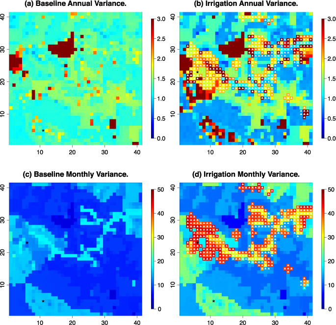
Figure 3. Annual ((a) and (b)) and monthly ((c) and (d)) latent heat variance (normalized by the average value) for the baseline ((a) and (c)) and Irrigation ((b) and (d)) scenarios.
Download figure:
Standard image High-resolution imageIt is well know that irrigation, by design, increases ET. However, figures 3(b) and (d) show that irrigation also impacts seasonal and inter-annual variability. Increases in monthly variance correspond to farm locations. Because irrigation is only applied for six months of the year, summertime latent heat fluxes are elevated while winter fluxes remain the same, or are decreased with declining water table depths.
In general, the areas with the largest increases in annual variance also correspond to farms. This finding may seem counterintuitive as irrigation works to mitigate natural shortage and is inversely correlated to natural supply. However, because irrigation is applied at a set rate whenever the threshold is crossed, significant changes can be observed from year to year as the number of irrigation days varies. There are also several farms located along the river where annual variance stays the same or decreases. These locations are likely always energy limited so the addition of irrigation does little to impact variability. Non-farm areas with increases in annual variance correspond to areas with long-term pumping induced drawdown shown in figure 2.
Characterization of monthly and annual variability is expanded using Fourier transforms. Figure 4 shows power spectrum and wavelengths (1/f) for water table depth and latent heat flux at two points (one farm and one non-farm) for both the Baseline and Irrigation scenarios. Precipitation and temperature are also plotted for reference, although they do not vary with scenario. Linear models fit to wavelengths less than 0.8 years (∼10 months) with slopes equal to the spectral exponent (β) are overlaid on the spectrum. Additionally, break points are observed by changes in the slope of the linear model.
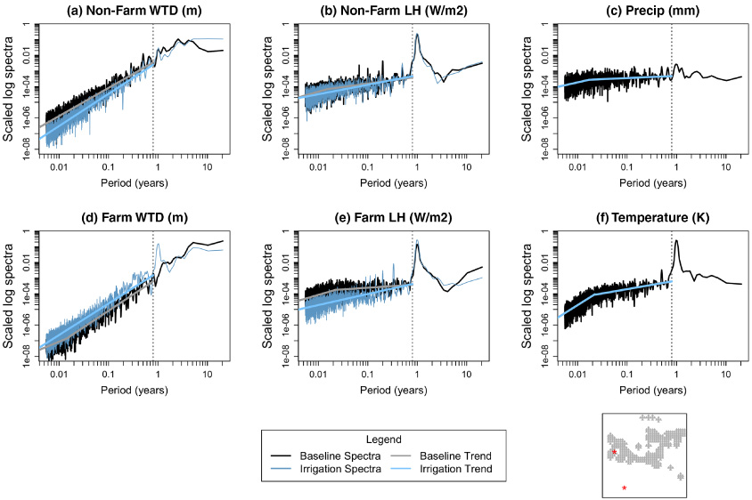
Figure 4. Periodograms of water table depth (WTD) and latent heat flux (LH) for a sample farm and non-farm point (shown in the inset map). Baseline (black) and Irrigation (blue) periodograms are overlaid with linear models fit to each scenario for periods less than 0.8 years (shown with vertical dashed line). Precipitation and temperature for the baseline case are also plotted ((c) and (f)) for reference.
Download figure:
Standard image High-resolution imageConsidering first the high frequency (periods less than 0.8 years) behavior for the Baseline scenario, plotted in black in figure 4, each variable displays unique temporal behavior. Water table depth has strong scaling even past the 0.8-year threshold used to fit trends. Latent heat displays temporal organization out to roughly one week (0.02 years) after which the slope is flatter and it behaves more like white noise. These findings are consistent with previous studies that showed decreased spectral power with longer wavelengths and longer persistence moving deeper into the subsurface (e.g. Amenu and Kumar 2005, Li and Zhang 2007, Pandey et al 1998, Schilling and Zhang 2012, Tessier et al 1996). Comparing model outputs to forcings, the precipitation log-spectrum is essentially flat (i.e. white noise) while temperature is more fractal with the strongest organization occurring at periods less than one week. The strong scaling behavior of water table depth highlights the basins ability to act as a fractal filter (e.g. Duffy and Gelhar 1985, 1986, Kirchner et al 2000, Little and Bloomfield 2010).
Given the declining slopes for latent heat flux, scaling exponents are not analyzed past 0.8 years, however, low frequency variability can still be observed in figure 4. Again focusing on the Baseline scenario, temperature and latent heat both have characteristic frequencies at one year (i.e. seasonal cycles). Water table depth and precipitation have much smaller annual peaks that are only slightly larger than the peaks around three and six years which could correspond to low frequency climate oscillations such as ENSO (∼3–9-year period of oscillation). This indicates that precipitation and water table depth experience more pronounced multi-year cycles, while for temperature and latent heat flux the annual cycle is much stronger than inter-annual variability.
Comparing behavior in figure 4 between scenarios, irrigation impacts frequency behavior in two ways; first by shifting the spectrum, and hence the relative importance of different frequencies, and second by changing spectral exponents. For the farm cell, the relative importance of low period (high frequency) variability is increased and a strong annual cycle is introduced. These shifts are countered by a decrease in the power of multi-year (low frequency) variability. Conversely for the non-farm point the relative importance of high frequency variability is decreased. At the farm location, β remains essentially unchanged with irrigation however, at the non-farm point there is a slight increase, indicating greater self-organization.
Irrigation also induces similar shifts in spectral power for latent heat flux. Again, the annual cycle is amplified with irrigation for the farm cell, however, unlike water table depth, this is countered by a decrease in the relative importance of high frequency variability. Also, the spectral exponent increases for periods ranging from one week out to 10 months (0.02–0.8 years) for the farm cell. In the Baseline scenario, the scaling diminishes after one week however, with irrigation there is no break point out to the 0.8-year fitting range. Unlike water table depth, significant impacts from irrigation are not observed for latent heat in the non-farm cell. This is consistent with earlier figures that showed water table impacts extending far beyond the points of pumping but localized latent heat changes.
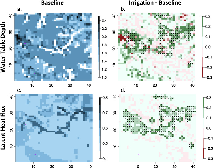
While the two points shown in figure 4 are instructive examples, they are not necessarily representative of behavior across the domain. In fact, analysis shows that temporal behavior is spatially organized. Figure 5 maps the spectral exponents of water table depth and latent heat flux for the Baseline scenario along with differences between the Irrigation and Baseline scenarios.
Figure 5. Scaling exponents of water table depth (a) and latent heat (c) for the baseline scenario and differences in scaling exponents (Irrigation–Baseline) for the same variables ((b) and (d)).
Download figure:
Standard image High-resolution image
Figure 5(a) shows decreased temporal organization of water table depth along the river where the groundwater is most closely connected to the surface. Furthermore, locations along the river have breaks in scaling ranging from 10 to 30 days, whereas much of the rest of the domain exhibits consistent scaling with no break points. These findings agree with Schilling and Zhang (2012) who observed a clearer spectrum with a single slope in wells located in upland areas away from the river. The range of slopes from ∼1 to 2.5 is also in good agreement with the β values of 1.87–2.26 observed by Schilling and Zhang (2012) in upland wells. Previous studies have observed declining scaling within the riparian zone moving from the river to the floodplain over the span of hundreds of meters (Li and Zhang 2007, Little and Bloomfield 2010, Schilling and Zhang 2012). However, this finding cannot be compared here due to the lateral resolution of 1 km.
Spectral exponents of latent heat flux are uniformly lower than water table depth (maximum of ∼0.8 compared to ∼2.5 for water table depth). The β values presented here are lower than the D'Odorico and Rodriguez-Iturbe (2000) simulated values of 1.5 and 2.18 for ET. It is likely that these differences result from different spatial aggregation and vegetation types. Still, the decrease in scaling exponents from groundwater to ET is consistent with Li and Zhang (2007) who observed decreased scaling from rainfall to streamflow to groundwater as a result of the dampening effect of land surface soils and aquifers. Breaks in scaling ranging from ∼4 to 10 days are observed across the domain except along the river where scaling is characterize by a single slope. Again this finding is consistent with break points observed in other studies and is likely related to 16 day maximum life time of planetary atmospheric structures (e.g. Pandey et al 1998). It is also interesting to note that along the river the exponents for water table depth and latent heat flux are the closest to one another. This highlights differences in scaling behavior between groundwater and surface water. When the groundwater is shallow and hence closely interacting with the surface, its scaling properties are more similar to surface variables such as latent heat flux.
In addition to the distinct scaling behavior observed along the river, subtle spatial patterns throughout the domain are qualitatively consistent with variations in hydraulic conductivity and land cover (see figure S1, available at stacks.iop.org/ERL/9/034009/mmedia). Latent heat flux appears to have slightly greater temporal organization for savanna as compared to grasslands. While water table depth displays increased scaling in high conductivity areas. Previous studies have observed different scaling behavior between boreholes in the same aquifer (e.g. Li and Zhang 2007, Little and Bloomfield 2010). However, relationships between scaling exponents and aquifer heterogeneity have not been established (Zhang and Li 2005). While the variations observed in figure 5 appear to display spatial patterns, additional research is required to determine whether the small differences represent significant changes in scaling. Also, future work should investigate the impact of crop choice on scaling behavior within the irrigated areas.
Figures 5(b) and (d) illustrate the impacts of irrigation on temporal self-organization across the domain. Increased scaling is generally shown for both water table depth and latent heat flux around irrigated areas. Water table depths have larger increases but impacts are heterogeneous. Impacts to latent heat flux are generally more homogeneous within farm cells, except along the river where values are unchanged, likely due to the minimal irrigation applied. Changes in the scaling behavior of both variables indicate increased temporal organization both in the surface and the subsurface. Although additional research is required to understand the exact mechanisms for this change, it could be explained by Zhang and Li (2006) who noted larger scaling coefficients when forcing a one-dimensional groundwater model with exponentially correlated rather than white noise recharge. Here pumping and irrigation are tied to subsurface water content. Because soil moisture is temporally self-organizing, the pumping signal imposed on the groundwater is not white noise and has temporal behavior that varies with soil moisture. Therefore, in the irrigation scenario, the white noise precipitation signal is augmented by a temporally organized irrigation signal.
4. Conclusions
The primary finding of this analysis is that irrigation changes the fundamental temporal behavior of water table depth and latent heat flux in the natural system. Temporal dynamics are an important consideration for water management because system reliability is largely controlled by natural variance. If irrigation changes the variability of the natural system this could have implications for vulnerability and sustainability. Frequency analysis at a farm point shows that irrigation increases the relative importance of high frequency variability in water table depths while decreasing inter-annual variability. At a non-farm point the shifts are reversed with decreased high and increased low frequency variability.
Scaling behavior demonstrates temporal self-organization consistent with previous research showing that aquifers act as fractal filters (e.g. Duffy and Gelhar 1985, 1986, Kirchner et al 2000, Little and Bloomfield 2010). In keeping with Li and Zhang (2007) we find stronger scaling behavior in water table depth than latent heat flux. Scaling exponents decrease with increased wavelengths. Latent heat flux has clear breaks in scaling at ∼4–10 days consistent with atmospheric time scales noted in previous analysis (e.g. Pandey et al 1998).
This research goes beyond previous work by demonstrating clear spatial patterns in temporal behavior of water table depth and latent heat flux. Water table and latent heat coefficients are most closely related in cells along the river indicating groundwater–surface water connections. Further from the river coefficients appear to differ with hydraulic conductivity but additional research is required to determine whether changes are statistically significant.
Finally, we present spatial differences in temporal organization resulting from pumping and irrigation. In general, irrigated areas have increased scaling coefficients for both water table depth and latent heat flux. This shows that water management operations increase persistence in both the groundwater and surface water systems and expand the area where the two are closely connected. Additional research is required to understand causality, but the findings of Zhang and Li (2006) indicate that increased scaling could result from temporally correlated forcings.
Acknowledgments
The material presented is based on work supported in part by the National Science Foundation through its ReNUWIt Engineering Re- search Center (www.renuwit.org; NSF EEC-1028968). Additional funding was provided by the National Science Foundation through its Climate Change Water and Society (CCWAS) Integrated Graduate Education and Research Traineeship (IGERT) program (http://ccwas.ucdavis.edu/; DGE-1069333). This material was based in part upon work supported by the National Science Foundation (NSF) under Grant No. WSC-1204787. Computational resources were provided by the Golden Energy Computing Organization at the Colorado School of Mines using resources acquired with financial assistance from the National Science Foundation and the National Renewable Energy Laboratory.