
Abstract
Current emissions inventories of black carbon aerosol, an important component of PM2.5 and a powerful climate altering species, are highly uncertain in both space and time. One of the major and hardest to constrain sources of black carbon is fire, which comes from a combination of forest, vegetation, agricultural, and peat sources. Therefore, quantifying this source more precisely in both space and time is essential. While there is a growing body of work on this topic, the best estimations generally underestimate measurements by integer factors. In this work, 12 years of measurements from 2000 through 2012 of AOD from the MISR satellite and AOD and AAOD from the AERONET network, are used to evaluate the aerosol climatology from Southeast Asian fires. First, the fires in Southeast Asia are uniquely characterized in both space and time to reveal two major burning regions: one with a regular inter-annual and intra-annual distribution, and the other with an irregular inter-annual and somewhat variable intra-annual distribution. These patterns correspond well with regional and local measurements of both composition and meteorology. Using these newly developed relationships, a new temporally and spatially varying set of black carbon emissions is developed. Finally, the best fits with the various measurements yield an annual average value for black carbon emissions due to fires bounded by the range 0.36–0.54 Tg yr−1, with the amount in the year of the greatest fires being bounded by the range 1.2–1.8 Tg yr−1. These magnitudes are significantly higher and differently distributed in space and time when compared with current inventories, and therefore are expected to have a significant impact on regional particulate loadings and the global climate system.
Export citation and abstract BibTeX RIS

Content from this work may be used under the terms of the Creative Commons Attribution 3.0 licence. Any further distribution of this work must maintain attribution to the author(s) and the title of the work, journal citation and DOI.
1. Introduction
Southeast Asia has been impacted the past 3–5 decades by widespread and ubiquitous fires (including but is not limited to forest fires, vegetation, agricultural fires, and peat fires) [1]. Due to large amounts of rainfall and the relatively moist surface, fires in this region typically occur during the local dry season [2]. These fires are clearly anthropogenic in nature, with large scale usage of fire for agriculture including rice, sugar, palm, rubber, and pulp, further combined with land clearance to accommodate a rising urban population [3, 4]. Some of the past fires in this region have been sufficiently intense and had wide enough spatial coverage to have significantly contributed to the regional-scale average aerosol optical depth (AOD) and surface PM2.5 (the total mass concentration of all particles with diameter smaller than 2.5 μm) levels [5–7].
One of the major aerosol species emitted by fires, black carbon (BC), is produced due to incomplete combustion. BC impacts both air quality and the climate system; it is a component of PM and hence impacts people's health, while also strongly scattering and absorbing solar radiation, impacting the climate. It has shown that BC alters the net energy budget of the Earth at the top of the atmosphere, although the exact value is not yet known (although always a net warming effect) from 0.25 to 0.9 W m−2 [8–15]. Furthermore, BC directly heats the atmosphere by uniquely absorbing visible sunlight. The combination of scattering and absorbing causes a unique impact on the energy budget: simultaneous cooling and heating. This has been shown to lead to large-scale changes in circulation and precipitation patterns [13–15].
Being able to quantify fires is challenging given that the observed fires persist in different parts of Southeast Asia during different times of the year, with the length and location of the burning period not necessarily following a regular pattern. There are multiple influences from the region's large-scale meteorology, which is characterized by two Monsoons, and how these Monsoons are modulated further by such regional phenomena as El Nino and the Indian Ocean Dipole. Overall, this leads to a diverse set of conditions in which there is a large amount of variation, on both inter-annual and intra-annual time scales, about the climatological mean for rainfall, surface radiation, and wetness [4, 16–19]. Additionally, there are linkages between the large-scale dynamics and the fires themselves, such that the particles from the fires are capable of altering and influencing the large-scale dynamics and precipitation itself [20]. Finally, Southeast Asia is heavily cloud covered throughout the year, leading to problems with using remote sensing to directly measure or detect fires [21].
Due to the issues raised here, previous efforts at using fire hotspot measurements to determine the extent and magnitude of emissions in Southeast Asia [1, 22–24] tend to underestimate the total number of fires, their duration, and intensity, all leading independently to an underestimation of the ultimate BC emissions. The method and data used in this work will present an alternative approach, from a top-down perspective, to independently and uniquely define the interannual and intraannual spatial and temporal patterns of Southeast Asian fires. Furthermore, the emission of BC due to these fires is quantified in an objective manner. All of these results are based on data from the MISR satellite and the ground-based AERONET and NOAA networks, over the period from 2000 to 2012, as well as a state-of-the-art model of atmospheric aerosol chemistry and physics.
2. Methodology
2.1. MISR, AERONET, and NOAA data
The particular region of interest, herein referred to as Southeast Asia, is bounded by 15S, 23N, 90E, and 130E. Twelve years of monthly average remotely sensed AOD measurements (March 2000 through March 2012) are obtained from the Multi-angle Imaging SpectroRadiometer (MISR) instrument on the Terra satellite to provide a remotely sensed AOD climatology [25].
This paper uses monthly average AOD level 3 data, which is cloud screened, resolved spatially to 0.5° × 0.5°, and includes all sources of AOD at 555 nm. Data from all of the available at optical bands (440 nm, 555 nm, 660 nm) and 1 infrared band (1010 nm) were used and the differences in the climatology and variance between the different optical bands were minimal. Furthermore, the results of the EOF analysis on the various different bands produce end products that are roughly identical in space and time. Furthermore, MISR is capable of providing a relatively precise spherical only AOD aerosol product, which is one way to attempt to account for highly non-spherical cirrus contamination of the AOD signal over this region [26]. A similar analysis of the climatology and variance, using the variance maximizing EOF analysis technique, as explained in the next section, on this product also produces a product that is nearly identical. Therefore, the results of this paper are all based on the total AOD from the 555 nm band, which has an average value and variance given in figure 1.
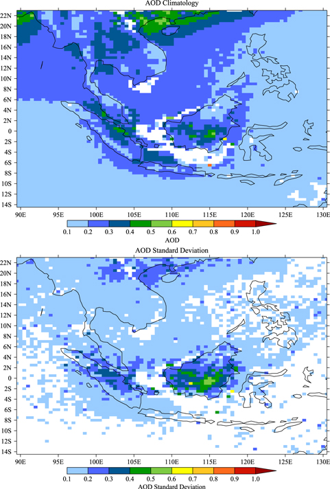
Figure 1. Climatology and standard deviation of MISR AOD over Southeast Asia as retrieved from March 2000 through March 2012, both of which were computed by first taking the monthly average values and then either averaging or computing the variance from these values. White regions are those in which there is either no data available (as shown by the AOD climatology) or where the values are less than 0.1 (regions of the standard deviation which are not also white in the AOD climatology).
Download figure:
Standard image High-resolution imageEvaluation of the analysis of the MISR AOD data and quantitative approximation of the implied BC emissions are done using data from the AErosol RObotic NETwork (AERONET) [27] and a surface measurement station from the NOAA Earth System Research Laboratory/Global Monitoring Division Network (NOAA) [28]. AERONET is a ground-based network that provides a measure of AOD and an approximation of the single scattering albedo (ω) (the fraction of the Sunlight scattered). Since there are known issues with AERONET not being able to compute ω correctly at low AOD values, only data corresponding to an AOD greater than 0.4 were included [29]. Since AERONET is used to ground truth MISR AOD, the correlations found are likely to be real. NOAA is a ground-based network that provides a measure of particulate absorption at the surface, given as  (m−1). Furthermore, data from both AERONET and NOAA have already been shown to be reliable in terms of providing an estimation of the emissions of BC within a bound of uncertainty when applied in conjunction with a set of forward model runs, as demonstrated by Cohen and Wang [30]. In this work it was demonstrated that the absorbing aerosol optical depth (AAOD) is a good way to quantify BC, since it is comprised of only three components: BC, dust, and absorbing OC. In this region of the world, the impact of dust is minimal, and the modeling system is capable of calculating the small amount of absorption due to OC (always less than 5%) which it then can subtract off from the overall model results [30], leaving BC as the only remaining constituent.
Combining these measures in equations (1a) and (1b) allows an approximation of the radiation absorbed, the AAOD from AERONET and with the inclusion of Zsurf, the model height of the surface layer, from NOAA, as in [30].


The geographic locations of the AERONET stations (and the co-located NOAA station at Lulin) used in this work are given in supplementary figure 1. The portions of the time series relevant to this work are given for monthly average AERONET AOD and NOAA absorption from 2003 through 2012 in figure 2(a) and for monthly average AAOD from 2003 to 2005 in figure 2(b).

Figure 2. (a, b) Time series of monthly average AERONET AOD (2000 to 2012) and NOAA absorption (2006 to 2012) (top) and AERONET AAOD (2002 to 2005) (bottom) used in this study.
Download figure:
Standard image High-resolution image2.2. Empirical orthogonal functions (EOF)
To correctly measure the contribution of fires to the total AOD, the approach needs to be able to capture both the large variance in AOD during the local dry phase and the small variance in AOD during the local wet phase. Given the nature of this problem, the method of EOF [31] is applied. This technique uniquely decomposes the temporally and spatially varying AOD measurements into a set of orthogonal standing signals that contribute the maximum variance of the underlying dataset. Additionally, this method provides a test for the efficacy of any model results of AOD, which must produce a similar pattern to those produced from the MISR AOD, if they are to be considered a reliable representation.
This procedure guarantees that each mode is orthogonal, and therefore represents a unique phenomenon in space and time. Sorting by the value of trace (TiSiT) (where Ti and Si are the temporal and spatial decomposition corresponding to the ith mode of the variability of the underlying dataset), leads to the conclusion that only the first two modes are sufficient to effectively reproduce the variability of the underlying data (49.7% and 19.2% respectively). Details of the definitions and derivation of the EOF method are given in supplementary text 1.
2.3. MIT-AERO-URBAN model
The final component to compute the quantity of fire emissions and analyze their spatial and temporal performance in Southeast Asia is a suitable global model that can simulate values of AOD and AAOD from BC and OC emissions, and further derive quantities which can then be compared against MISR and AERONET measurements. For this work, we have chosen to use the MIT AERO-URBAN model [9, 12], a state of the art modeling system that simulates the chemistry, physics, and transport of aerosols at regional to global scales. Details of this model are given in supplementary text 3, and include: circulation driven by a 3D general circulation model [32] using NCEP reanalysis to make comparisons against surface measurements, a coupled treatment of aerosol physics (2-moment) and chemistry (internal and external mixtures) [12], and the ability to handle subgrid processing due to unique conditions in urbanized regions (which constitute a large amount of the emissions in this part of the world) [9, 33].
3. Results
3.1. Southeast Asian AOD climatology
The EOF analysis method when applied on the MISR AOD dataset reveals two major regions of variability in the observations table 1. The more variable 'southern region' is defined by a time series given by the vector T1 and a geospatial pattern given by the matrix S1 shown in figures 3(a) and (b). On the other hand, the less variable 'northern region' is defined by a time series given by the vector T2 and a geospatial pattern given by the matrix S2 respectively displayed in figures 4(a) and (b).
Table 1. Statistical results presented in the paper. The top half concerns analysis of the MISR AOD data over the period from March 2000 to March 2012, while the bottom half concerns analysis of the model runs of the different emissions scenarios over the period from January 2002 to December 2005. The left hand column specifies the comparison of interest, the central column shows the results for the 'southern region', and the right hand column shows the results for the 'northern region'.
| Statistic of interest | Result in southern region (S1, T1) | Result in northern region (S2, T2) |
|---|---|---|
| Results based on MISR AOD data from 2000–2012 | ||
| Percent contribution to variance of MISR AOD | 49.7% | 19.2% |
| Correlation between MISR AOD averaged over Si and Ti | R2 = 0.98 | R2 = 0.97 |
Correlation between AERONET AOD, NOAA  and Ti and Ti |
Singapore: R2 = 0.45 | Mukdahan: R2 = 0.70 Chiang Mai: R2 = 0.83 Pimai: R2 = 0.64 Vientiane: R2 = 0.50 Bac Giang: R2 = 0.46 Ubon Ratch: R2 = 0.76 Nghia Do: R2 = 0.69 Dongsha: R2 = 0.43 Hong Kong: R2 = 0.42 Lulin (AOD): R2 = 0.63 Lulin ( ): R2 = 0.64 ): R2 = 0.64 |
| Cutoffs for Si and Ti | S1 = .02 | S2 = .02 |
| T1 = 7.0 | T2 = 5.2 | |
| Difference between MISR average AOD and MISR AOD over Si/Ti | RMS = 0.45 | RMS = 0.34 |
| Years of significant fires | 2002, 2004, 2006, 2008, 2009 | 2000, 2001, 2002, 2004, 2005, 2006, 2007, 2008, 2009, 2010, 2011, 2012 |
| Results from model runs under different emissions scenarios from 2002–2005 | ||
| Correlation between model AAOD averaged over Si and Ti computed from MISR AOD | EF = 0.3: R2 = 0.69 KF: R2 = 0.07 AEROCOM: R2 = 0.40 EF = 0.2: R2 = 0.65 | EF = 0.3: R2 = 0.73 KF: R2 = 0.44 AEROCOM: R2 = 0.59 EF = 0.2: R2 = 0.73 |
| Percentage overlap of model region Si with MISR region Si | EF = 30%: 70% KF: 0.0% AEROCOM: 44% EF = 20%: 70% | EF = 30%: 85% KF: 15% AEROCOM: 76% EF = 20%: 85% |
| Difference between AERONET AAOD and model AAOD | — | EF = 0.3: RMS = 0.069 KF: RMS = 0.071 AEROCOM: RMS = 0.109 EF = 0.2: RMS = 0.069 |
| Difference between AERONET AAOD climatology and model AAOD | EF = 0.3: RMS = 0.026 KF: RMS = 0.028 AEROCOM: RMS = 0.034 EF = 0.2: RMS = 0.026 | EF = 0.3: RMS = 0.035 KF: RMS = 0.049 AEROCOM: RMS = 0.086 EF = 0.2: RMS = 0.036 |
Difference between NOAA  climatology and model climatology and model 
|
— | EF = 0.3: RMS = 1.8 × 10⁻⁶ KF: RMS = 2.4 × 10⁻⁶ AEROCOM: RMS = 3.5 × 10⁻⁶ EF = 0.2: RMS = 1.7 × 10⁻⁶ |
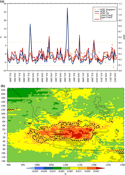
Figure 3. (a, b) Results of the EOF analysis performed on the MISR AOD data from 2000–2012. The upper plot contains the time series of the first principal component (T1) (solid red), MISR AOD averaged over the portion of S1 bounded by the dashed line (solid blue), MISR AOD averaged over all of Southeast Asia (dash-dot light red), and AERONET AOD from Singapore (dotted squares). The lower plot contains the spatial distribution of the first principal component (S1), with the region corresponding to the cutoff value bounded by thick dashed lines. Small x's indicate locations where there was not enough data to successfully perform the EOF analysis.
Download figure:
Standard image High-resolution image
Figure 4. (a, b) Results of the EOF analysis performed on the MISR AOD data from 2000–2012. The upper plot contains the time series of the second principal component (T2) (solid red), MISR AOD averaged over the portion of S2 bounded by the dashed line (dash-dot light red), MISR AOD averaged over all of Southeast Asia (solid blue), AERONET AOD from stations inside both the burning areas and the corresponding domain (S2) (dotted lines), AERONET AOD from stations which are outside the burning areas and still inside S2 (dashed lines), and NOAA absorption outside the burning areas and still inside S2 (thin blue). The lower plot contains the spatial distribution of the second principal component (S2), with the regions corresponding to the cutoff value bounded by thick dashed lines. Small x's indicate regions where there was not enough data to successfully perform the EOF analysis.
Download figure:
Standard image High-resolution imageThese mathematical findings compare well with an analysis of the AOD climatology over Southeast Asia, which leads to three general observations. First, that there are parts of this region with a very high amount of variation. Second, much of this variation (annually for Continental Southeast Asia: Myanmar, Thailand, Cambodia, Laos, and Vietnam, and frequently for the maritime continent: Indonesia, Malaysia, Singapore, and Brunei) corresponds with the locally driest phase of the Monsoon, supplementary figure 2 [34]. Third, regions corresponding with known urbanization or high population density including Java, Bangkok, Hanoi, Ho Chi Minh City, the Western coast of Malaysia, and Singapore, consistently have a high AOD and a relatively low variability throughout the year. What variability exists is due to large external sources such as fires from upwind regions. Therefore for the remainder of this paper, the emissions from these urban areas will be treated as being time-invariant.
Comparing the average of MISR measurements over the respective domains S1 and S2 as a function of time, against the values of T1 and T2 shows that the EOFs yield highly representative results table 1. It is clear that throughout the 12 years, all years with a known high AOD event are captured by T1 and T2, and years with no high AOD events are correspondingly not captured figures 3(a) and 4(a). On the other hand there is weak to no correlation (R2 < 0.07) between the average AOD over all of Southeast Asia with both T1 and T2, confirming that the regions S1, S2, over the time series T1, and T2 effectively and uniquely reproduce (R2 = 0.98 and R2 = 0.97 respectively) the variability of the MISR climatology (49.7% and 19.2% respectively).
3.2. Details over the maritime continent
The southern region (S1 and T1) corresponds to the maritime continent, which includes many regions where the land is being rapidly cleared by burning for agriculture and urban expansion, such as Sumatra, Borneo, and Peninsular Malaysia. As shown in figure 3(a), T1 correlates reasonably with AERONET measurements in Singapore (R2 = 0.45), which is interesting, given the difficulty of constructing such a relationship in this region for three reasons: the lack of a very long time series, the frequent contamination of measurements due to high cloud variability, and the lack of other measurement sites also in the outflow from fires [35].
Three important characteristics are found in the temporal pattern of this contribution to the variance when an appropriate cutoff supplementary text 2 is chosen table 1. First, there is strong inter-annual variability, with only some of the years (2002, 2004, 2006, 2008, and 2009) contributing to S1 and T1 figure 3(a). Second, the strength of the signal in the various fire years varies in intensity from a relative minimum in 2009 to a relative maximum in 2006 figure 3(a). Third, the duration of the fires also varies from 1 month in 2004, 2008, and 2009 to 2 months in 2002, and 3 months in 2006.
One rationale for this inter-annual variability is that in some years the onset of the wet phase of the monsoon in this region arrives at different times, as shown by the average precipitation over S1 as measured by the TRMM satellite supplementary figure 2. A second reason for inter-annual variability is attributed to the effects of El-Nino (as given by ENSO Precipitation Index, as computed from TRMM data [36]), which is correlated with some of the significant peaks in T1 (2002, 2006, and 2009). However, not all years (2004 and 2008) are explained by the above two phenomena, and therefore, since the other remote factors are considerably less important in terms of variance contribution in this region [4], localized factors such as convection or anthropogenic disturbance must also make an important contribution.
3.3. Details over continental Southeast Asia
The northern region corresponds to the continental portion of Southeast Asia (S2 and T2), and describes the time-varying emissions from known agricultural and land-clearing fires in Thailand, Myanmar, Laos, Cambodia, and Vietnam. T2 correlates well with AOD from AERONET at multiple stations table 1, 7 of which are located in fire burning areas figure 4(a) (dotted lines) as well as 3 of which are located far downwind from the burning areas figure 4(a) (dashed lines). Furthermore, there is also good correlation between T2 and surface absorption measurements from the NOAA station at Lulin, also located far downwind from the burning areas figure 4(a) (blue line). The strong correlations with T2 (R2 ranges from 0.42 to 0.83, with a median of 0.64) and the geographic reach of S2 indicate that the EOF is both representative of the aerosol climatology and that aerosols emitted in this region transport far from their source.
The northern region has two significant characteristics that can be found when an appropriate cutoff supplementary text 2 is chosen table 1. First is that there is a recurring annual signal, except for 2003. Second, that the length and strength of the fire signal is roughly similar from year to year. The fires peak in March and last for one month, except for in 2005 and 2010, in which they continue through April.
A comparison with the rainfall time series as averaged over the land areas of S2 supplementary figure 2 shows that the fires will start near the end of the local dry period, with roughly the same start-time each year. Secondly, the inter-annual variability associated with El Nino seems relatively unimportant in this region. Thirdly, it is important to note that there is significant variability in the arrival of the wet season. While the average precipitation is low every year in February, March, and April over S2 (defined as being below the annual climatology over the land-based portion) there are 2 years in which February, 4 years in which March, and 7 years in which April is not extremely dry over the land portion of S2 (defined as being below the mean April climatology over the land region), as well as 2 years in which May is still relatively dry over the land portion of S2 (defined as being less than the mean April climatology over the land region plus 1 standard deviation). These findings are consistent with the fact that this region has many managed ecosystems that are systematically burned for recurring agricultural purposes, and therefore are designed to be as resistant as possible to large-scale changes in the precipitation system [37, 38].
4. Discussion and conclusions
4.1. Fire emissions in space and time
The established spatial and temporal patterns obtained from the EOF methodology applied to the MISR data successfully reproduce the AOD over Southeast Asia due to emissions of aerosols from fires in this region table 1. Furthermore, these results provide an objective basis set upon which a quantitative measure of the goodness of fit in space and time of any model simulation of the aerosols associated with fires from this region. Additionally, the regions within S1 and S2 over land effectively constrain the spatial regions from which fire emissions occur, and when modulated in time by T1 and T2, form a new emissions field for the BC associated with these fires. All emissions due to fires occur over land areas, and therefore the values within the regions S1 and S2 which occur over the ocean are a direct consequence of the transport of these emissions and any subsequent chemical and physical changes which these emissions have undergone in situ.
To develop this new time-varying inventory of BC emissions, a temporally and spatially varying pattern EM is determined in equation (2), such that the value is representative of the magnitude of variation contributed to the overall dataset, or zero if it is below the respective cutoff table 1. This pattern is then used as the basis of the weights and locations of fire emissions in both space and time over land.

In addition to fire sources, EM may also increase due to certain chemical and physical sources and sinks of AOD in the atmosphere. Any climatologically relevant changes in aerosol plume-rise height, relative humidity, and changes in rainfall need to be considered. However, there is no evidence that any of these have changed significantly over the 12 years analyzed to alter the variance of the spatial distribution on these scales, and the few impacts of the changes in the Monsoon arrival only modulate the temporal pattern during some of the years, but not others.
It is also possible that secondary aerosol production could lead to an increase in variance, but only in the case where a nonlinear interaction occurs between the time varying fire source and the local non-time varying urban source. This is found to occur in the case where smoke from fires is highly concentrated and passes over the plume from an urban area. In this case, the interaction of the smoke and urban plumes lead to the BC in the plume interacting with H2SO4 from the urban area [9, 33], leading to enhancement in the scattering and absorbing properties of the aerosols, inducing variability in the AOD field. This characteristic is observed around and downwind from Hanoi (as shown in a section of S2) and Singapore (as shown in a section of S1). However, since it is known that these cities do not burn within their boundaries, EM in these regions is set to zero.
It is these reasons that this work is only approximating the emissions of BC and not of other co-emitted species. The data on AAOD and absorbance provide a unique constraint to the contributions to absorption from this region, which are due to BC. If one were to also include the AOD it would still not be a unique problem to solve for the BC plus OC or total Particulate Matter due to the fact that both OC and Sulfate would need to be simultaneously constrained. Such nonlinear processing as talked about above would make this currently impossible, and it is for this reason that only BC is considered in this work.
Assuming that a fixed percentage, EF, of the total non-time varying BC emissions, EBC , for Southeast Asia is due to fires, allows various emissions scenarios to be developed. This study chooses a low and high value of EF = 20% and EF = 30%, respectively, while EBC = 1.73 Tg yr−1 is taken from the top-down constrained estimate by Cohen and Wang [30]. These numbers are sufficiently large to bound the results, and yet are still within the error bounds given in Cohen and Wang [30].
The final assumption is that the quantity of total non-fire emissions, EBC , is roughly time-invariant. In Southeast Asia, although there is economic growth and expansion of urbanization, these changes happen on time scales longer than those relevant to the burning season changes.
Combining these assumptions, the emissions are derived as equation (3).
4.2. Modeling with new fire emissions
In addition to the two newly derived time-varying fire emissions inventories (EF = 20% and EF = 30%), two other emissions datasets commonly used by the community, the Kalman filter (KF) derived emissions from [30], and a combination of the fire hotspot based inventory GFED [39] and the urban emissions inventory AEROCOM [40] are also tested. All four scenarios were run in the forward modeling system MIT-AERO-URBAN [9], using the same multi-year meteorology from October 2001 to December 2005 (October 2001 to December 2001 is for spin-up only), to compute the AAOD (supplementary text 3). The results were then analyzed using the same EOF technique as the MISR data.
A temporal comparison of model AAOD derived T1 and T2 are compared against T1 and T2 derived from MISR AOD. The cases EF = 30% (R2 = 0.69 southern region and R2 = 0.73 northern region) and EF = 20% (R2 = 0.65 southern region and R2 = 0.73 northern region) capture both inter-annual and intra-annual variation table 1, figures 5(a) and (b). The AEROCOM case (R2 = 0.40 southern region and R2 = 0.59 northern region) captures the climatological high fire timing, but not its entire length or inter-annual variation. The KF case is generally poorly correlated. Overall, all of the results perform less well over the southern region due to extensive cloud coverage over land which likely interfere with a full measure of the AOD's variability in these regions figure 5(a).

Figure 5. (a, b, c) Comparison of the time series of the modeled AAOD fields under the different emissions cases. The top plot is the time series of the respective T1 values of all modeled AAOD fields (EF = 30% dotted red, KF dashed light blue, AEROCOM dash-dot orange, EF = 20% dash-dot-dot-dot light blue), the AERONET AAOD climatology at Singapore (thin purple) and the Observed MISR T1 (solid red). The middle plot is the time series of the respective T2 values of all modeled AAOD fields (same colors as top panel), AERONET AAOD (dashed with points) at stations in S2, and the observed MISR T2 (solid red). The bottom plot is the time series of the respective T2 values of all modeled AAOD fields (same colors as top panel), NOAA absorption at Lulin (thin blue), and the observed MISR T2 (solid black).
Download figure:
Standard image High-resolution imageNext, the geographic distribution of the fire emissions patterns are compared between the model derived and MISR computed S1 and S2. An excellent correlation for EF = 30% and EF = 20% in both domains is found (northern 85%, southern 70%), while AEROCOM produces a reasonably good correlation in the northern region only (northern 76%, southern 44%). The KF case does not reproduce the spatial distribution well in either domain (northern 15%, southern 0%) table 1 and figure 6. Again, the southern region is less well represented across the board, and only successfully so in the EF = 30% and EF = 20% cases figure 7.

Figure 6. (a, b, c, d) The top left plot contains the spatial domain of EF = 0.3 S2, the top right plot contains the spatial domain of KF S2, the bottom left plot contains the spatial domain of AEROCOM S2, and the bottom right plot contains the spatial domain of EF = 0.2 S2. In all plots, thick dashed lines bound the cutoff value.
Download figure:
Standard image High-resolution image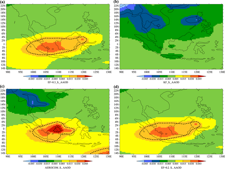
Figure 7. (a, b, c, d) The top left plot contains the spatial domain of EF = 0.3 S1, the top right plot contains the spatial domain of KF S1, the bottom left plot contains the spatial domain of AEROCOM S1, and the bottom right plot contains the spatial domain of EF = 0.2 S1. In all plots, thick dashed lines bound the cutoff value.
Download figure:
Standard image High-resolution image
Finally, to quantify how closely the modeled atmospheric fields of BC match measurements, comparisons were made directly with the four AERONET stations that had measurements of AAOD figure 2(b). Computing the root mean square error leads to the conclusion that the cases EF = 30%, EF = 20%, and KF all produce a similarly good result over the entire four year model period table 1 and figure 5(b). The major improvement between the EF = 30% and EF = 20% on one hand and the KF case on the other occur during the high fire periods, with both EF cases producing a lower root mean square error. In general, EF = 30% matches the high AAOD stations well, while EF = 20% matches the low AAOD stations. And while the AEROCOM case performed better than the KF case in space and time, as is shown here, the AEROCOM case significantly underestimates AAOD throughout the entire time series.
Given that there is only a small amount of data at two of the northern stations, Hong Kong and Pimai that overlaps with the modeled period, and that the Singapore AAOD and NOAA data do not correspond to the modeled time period, a climatology of these four data sets are derived as shown in figure 5(a) for Singapore, figure 5(b) for Hong Kong and Pimai, and figure 5(c) for the NOAA data at Lulin Mountain. In each case the data has been averaged month by month over all of the years in which there is data present. Each of these datasets has a minimum of four years worth of overall data, leading to the climatological averages being representative of typical conditions: hence falling somewhere between a high fire and low fire year, especially so for Singapore in which the difference between years is greater.
The RMS error is computed between each of the model runs and these climatologies respectively and the results are found to be consistent. In all cases except for Singapore, EF = 30% and EF = 20% perform slightly better than the KF case and all perform much better than the AEROCOM case table 1. At Singapore, the noise of the climatology is larger and all three cases EF = 30%, EF = 20%, and KF perform roughly equally, while still all performing better than AEROCOM table 1. Further analysis with a Kalman filter or similar method would produce a better approximation [30], as would comparison with further surface measurements that are just starting to become available.
Given the results, it is clear that both EF = 30% and EF = 20% fit best with respect to time (inter-annually and intra-annually), space, and quantity. Furthermore, since they capture the lowest and highest measurements well, it is assumed that these two scenarios should bound emissions of BC from fires in Southeast Asia. Therefore, extending the results from the EF = 20% and EF = 30% case to the entire 12 year time series based on T1 (5 fire years) and T2 (12 fire years), leads to an annual average emissions of BC from fires in this region to be strictly bounded between 0.36 Tg yr−1 and 0.54 Tg yr−1. Similarly the inter-annual emissions of BC from fires is strictly bounded between 0.11 Tg yr−1 and 0.17 Tg yr−1 in the lowest year (2011) and is strictly bounded between 1.2 Tg yr−1 and 1.8 Tg yr−1 in the highest year (2006).
These values are a significant increase from current inventories, which place global annual BC emissions from all sources, burning and anthropogenic combined, from 7.662 Tg yr−1 [41, 42] to 17.8 Tg yr−1 [30]. The underestimation for Southeast Asia is sufficiently large that the annual average fire emissions of 0.36 Tg yr−1 to 0.54 Tg yr−1 is slightly larger than the annual average uncertainty bound of 0.38 Tg yr−1 for the total Southeast Asian BC emissions for all sources including urban activities and fires, which has already been shown in the same work to be statistically significantly higher than all other commonly used datasets for Southeast Asian BC emissions [30]. In fact, the maximum year emissions found here of between 1.2 Tg yr−1–1.8 Tg yr−1 is larger than the entire BC emissions for all sources including urban activities and fires, which was found to have an annual average value of 1.21 ± 0.38 Tg yr−1 (standard deviation) [30]. The GFED emissions dataset gives the annual average BC emissions for Southeast Asia plus India for all fire sources as 0.227 ± 0.118 Tg yr−1, which is clearly lower than our annual average value. Additionally, their maximum value for fire emissions over Southeast Asia plus India is 0.487 Tg yr−1, which is also considerably lower than the results found here.
Therefore, this set of results concludes that the underestimation of BC emissions due to higher burning years provides a significant increase in global BC emissions, even when compared with the error bounds given by Cohen and Wang [30]. Furthermore, the underestimation of BC emissions is important on a regional basis even in low burning years. Hence, by properly reproducing both the intra-annual and inter-annual variability, further significant improvements to estimates of global BC impacts on climate and concentrations of PM are expected.
Acknowledgments
This work was supported by the Singapore MOE's AcRF Tier 1 Grant (R-302-000-062-133) and the Singapore National Research Foundation (NRF) through a grant to the Center for Environmental Sensing and Monitoring (CENSAM) of the Singapore-MIT Alliance for Research and Technology (SMART). The author wants to thank all of the Principal Investigators of MISR, AERONET, and NOAA for making the data available. The author would also like to thank Chien Wang for his introduction to and practical advice on the use of the EOF methodology. Finally, the author would like to thank the three anonymous reviewers for their comments and suggestions that have helped to improve the paper.