

Abstract
Large-scale spatial population projections are of growing importance to the global change community. Spatial settlement patterns are a key determinant of vulnerability to climate-related hazards as well as to land-use and its consequences for habitat, energy use, and emissions of greenhouse gases and air pollutants. Few projections exist of spatial distribution at national or larger scales, and while recent efforts improve on earlier approaches that simply scaled or extrapolated existing spatial patterns, important methodological shortcomings remain and models have not been calibrated to nor validated against historical trends. Here we present spatially explicit 100-year projections for the continental United States consistent with two different scenarios of possible socio-economic development. The projections are based on a new model that is calibrated to observed changes in regional population distribution since 1950, corrects for distorting effects at borders, and employs a spatial mask for designating protected or uninhabitable land. Using new metrics for comparing spatial outcomes, we find that our projections anticipate more moderate trends in urban expansion and coastal settlement than widely used existing projections. We also find that differences in outcomes across models are much larger than differences across alternative socio-economic scenarios for a given model, emphasizing the importance of better understanding of methods of spatial population projection for improved integrated assessments of social and environmental change.
Export citation and abstract BibTeX RIS

Content from this work may be used under the terms of the Creative Commons Attribution 3.0 licence. Any further distribution of this work must maintain attribution to the author(s) and the title of the work, journal citation and DOI.
1. Introduction
Spatially explicit projections of the human population are of growing importance in the scenario-based assessment of global change, vulnerability, and sustainable development. Changes in the size and spatial distribution of the population, particularly in regions experiencing rapid growth and urbanization, will have significant ecological and socio-economic implications. Assessing these implications requires plausible alternative projections of spatial population distribution, and there is increasing demand for spatial projections that can be made consistent with widely used global change narratives describing changes in other characteristics of society that could affect spatial outcomes, such as economic development, policy changes, and changes in the energy system and demand for land. In turn, spatial population change can affect other aspects of society. For example, it is a significant driver of land-use/land-cover change, both directly through conversion to residential, commercial, and industrial uses, and indirectly as increased food demand drives conversion to agricultural uses [1–3]. Rapid urbanization in many world regions is a significant threat to protected areas, sensitive habitats, and biodiversity [4]. Projections of spatial change, consistent with alternative global change scenarios, are crucial to identifying potential future environmental hotspots [4, 5].
Cities and urban agglomerations exert significant pressure on climate, land, and hydrology at local, regional, and global scales [6]. Invariably, city growth and the corresponding expansion in urban land is driven by population growth. Rapidly improving satellite data has led to a substantial amount of recent parallel work related to defining and projecting the spatial extent of urban land-cover [6–8], work often informed by, or used as an aid in, projecting spatial population. In addition to land-use change, alternative forms of urban development have varying implications for energy demand and emissions [9, 10]. Projections of spatial emissions of greenhouse gases and air pollutants often rely explicitly on spatial population data [11, 12]. Similarly, estimates of both the size and spatial orientation of populations are crucial to planners that must ensure adequate access to food, water, energy, and public services while attempting to reduce vulnerability to climate-related hazards [13–16].
Most spatially explicit projections of the future population are carried out at the region or city scale, span short time horizons [17, 18], and use widely varying methodologies. At larger scales, there have been significant improvements over the past two decades in the quality and availability of gridded distributions of the existing population, including globally [19, 20]. To date, however, there are relatively few spatially explicit projections of future population distribution over large areas and long time horizons, and methods for producing such projections are in the early stages of development. Alternative assumptions regarding broad regional population change are an important component of the integrated scenarios that guide global change research, including the Special Report on Emissions Scenarios (SRES, [21]) from the Intergovernmental Panel on Climate Change (IPCC), as well as the newer Representative Concentration Pathways (RCPs, [22]) and the corresponding Shared Socio-economic Pathways (SSPs, [23]). Inherently these broad assumptions have local consequences, and variation in the spatial distribution of projected population change will result. Many of the existing large-area spatially explicit projections are scaled so that regional populations match the totals from the SRES scenarios [24, 25]; however, in most cases there is very little connection between projected patterns of spatial change and the qualitative narratives.
The majority of the existing large-scale spatially explicit projections are constructed using simple scaling techniques or trend extrapolation [24–26]. By definition these projections reflect a future world in which the spatial population structure does not change, or changes only through continuation of the most recent sub-regional trend. They have typically been used as a stop-gap measure [27] and reflect only a single, somewhat unlikely spatial pattern. More sophisticated methods have been developed that improve on these models. One approach is based on a correlation between a beta function describing the existing rank-size distribution of grid-cell population (at the national-level) and socio-economic variables [28]. While the model is global in nature, it does not project population for cells with an existing population density under 2 persons km−2; thus coverage is limited to roughly 44% of the Earth's land surface. Additionally, the methodology imposes the existing rank-size distribution on all future distributions (e.g., the most densely populated cell always remains so).
An alternative approach developed at the International Institute for Applied Systems Analysis (IIASA, [29]) uses a gravity-based model to produce global scenarios by allocating national-level projections of urban and rural population change to grid-cells according to a population potential surface, a commonly used tool in spatial interaction modeling. Gravity models, borrowed by geographers from the physical sciences (e.g., Newton's laws of gravitation and gravitational potential), seek to describe the movement of people, goods, and information over space and have long been traditional tools in geography and spatial demography. The population potential model is a type of gravity model commonly used to assess the accessibility or attractiveness of a place [30]. In this application potential for each grid-cell is calculated as a distance-weighted measure of the population in nearby cells, and projected change in population is allocated proportionally according to the potential surface. The model is limited in that it enforces a single pattern of spatial development (rapid expansion/population dissemination) across all regions [31]. The US Environmental Protection Agency (EPA) produced two high-resolution projections for the continental United States [1] by projecting housing density across a high-resolution grid as a function of projected county-level population change, urban land-use, infrastructure, topography, and accessibility [32, 33]. Due to data constraints and consistency issues, the approach is not globally applicable.
Here we present a new model for producing large-scale spatially explicit future population scenarios that addresses several of the shortcomings in previous approaches. We use a population potential model [29] to downscale aggregate population projections, introducing free parameters into the model that can be calibrated to reflect patterns of spatial change in historical data and altered if desired to reflect varying assumptions regarding socio-economic futures. The model is applicable at varying scales of spatial analysis, treats urban and rural populations as separate yet interacting entities, and includes mechanisms for correcting edge-effects and limiting habitable land area. To illustrate, we present two 100-year spatial projections consistent with socio-economic scenarios widely used in climate change research: the A2 and B2 scenarios from the SRES storylines (see the supplementary information, SI, available at stacks.iop.org/ERL/8/044021/mmedia). We calibrate the model to observed spatial development over the period 1950–2000, and compare our results to those produced using the IIASA and EPA projection models. Finally, we introduce metrics that can be derived from our projections that are potentially of interest to the planning community and/or those interested in vulnerability.
2. Methodology
Beginning with a gridded distribution of the base-year population the model consists of five basic steps: (1) define the urban/rural proportional mix of the population within each grid-cell, (2) calculate an urban population potential surface, (3) calculate a rural population potential surface, (4) allocate projected urban population change to grid-cells proportionally according to their respective urban potentials, and (5) allocate projected rural population change to grid-cells proportionally according to rural potential. Steps 2–5 are then repeated for each time step.
The base-year distribution for the continental United States consists of roughly 53 000 1/8° grid-cells. Population data are transferred from polygons and points to grid-cells using census tracts, census populated places, and county-level data (see the SI). People are defined as urban or rural during the gridding process according to their census classification. Each grid-cell can contain both urban and rural populations. In this research 2000 served as the base-year, but for purposes of calibrating the model a gridded distribution of the 1950 population was constructed (see the SI).
Separate population potential surfaces are used to allocate projected urban and rural population change. However, both urban and rural population potential are calculated using the total existing population in each grid-cell. Potential for each cell is calculated as:
where vi is potential of cell i, ai is a cell-specific adjustment factor that removes boundary effects from the calculation of potential, li is the portion of each cell that is suitable for human habitation (see the SI), P is population within a grid-cell, d is geographic distance between two grid-cells, α and β are parameters, and j is an index of the m cells within a 100 km window around cell i (see the SI). Urban and rural potential are both calculated using equation (1), however the urban and rural values of α and β will vary due to the different historical evolution of urban and rural spatial patterns. The β parameter is a measure of the impact of distance on the contribution of nearby populations to potential, while the α parameter is indicative of the importance of local characteristics. We use historical urban and rural population change data to estimate separate urban and rural parameters.
The calibration procedure is constructed as an unconstrained minimization problem solved using the generalized reduced gradient (GRG2) algorithm [34]. We use gridded distributions of the 1950 urban and rural populations and project the 2000 distributions, deriving the α and β values that produce a best fit. Parameters are generated for each national or sub-national unit for which exogenous estimates of population change are to be downscaled (see table 1). For example, the A2 and B2 scenarios presented in this letter were constructed by downscaling projected urban and rural population change for each of the nine census divisions. For the A2 scenario we used parameter estimates derived from the south region, while estimates from each respective division were applied in the B2 scenario. The calibrated model predicts the population distribution in 2000 substantially better than either the IIASA methodology or proportional scaling (see the SI).
Table 1. Parameter estimates for the urban and rural populations at the national-level, for the four census regions, and for the nine census divisions.
| Region/Division | Urban | Rural | ||
|---|---|---|---|---|
| α | β | α | β | |
| National | 0.897 | 0.082 | 0.999 | 0.101 |
| Northeast | 0.965 | 0.094 | 0.977 | 0.097 |
| New England | 0.979 | 0.096 | 0.998 | 0.099 |
| Mid-Atlantic | 0.962 | 0.093 | 0.970 | −0.007 |
| Midwest | 0.913 | 0.081 | 1.006 | 0.094 |
| East North Central | 0.952 | 0.092 | 1.005 | 0.098 |
| West North Central | 0.879 | 0.079 | 1.014 | −0.017 |
| South | 0.830 | 0.071 | 1.001 | 0.101 |
| South Atlantic | 0.836 | 0.072 | 1.001 | 0.100 |
| East South Central | 0.816 | 0.068 | 1.001 | 0.098 |
| West South Central | 0.840 | 0.073 | 1.000 | 0.102 |
| West | 0.821 | 0.072 | 0.994 | 0.115 |
| Mountain | 0.795 | 0.065 | 0.994 | 0.114 |
| Pacific | 0.947 | 0.091 | 0.992 | 0.118 |
At each time step the projected change in urban and rural population is allocated separately across all grid-cells proportionally according to the urban and rural potential surfaces. If projected population change is negative, then the allocation of population loss occurs as proportional to the inverse of potential. Because potential is indicative of the relative attractiveness of each grid-cell it stands to reason that the least attractive places will experience proportionally larger losses during periods of decline. Neither the urban nor rural population in a grid-cell is allowed to become negative. Finally, a density ceiling of 35 000 km−2 is imposed (similar to the highest-density South Asian cities such as Singapore and Hong Kong).
Projections of the A2- and B2-divisional urban and rural populations were constructed using the interim state population projections produced by the US Census Bureau Population Division. Assuming linear change over the period 2030–2100 we aggregate divisional totals from the state-based projections, then scale the totals to meet the projected national totals for the A2 and B2 scenarios from the IIASA 2007 probabilistic world population projections. Divisional urbanization rates are assumed to converge on the projected national rates as projected in the IIASA scenarios, 93.8% for the A2 and 89.1% for the B2 (see the SI for national, regional, and divisional projections of urban and rural population).
3. One-hundred year spatially explicit scenarios for the continental United States
We produced scenarios for the continental United States (2000–2100) using different combinations of five factors: (a) the projected change in aggregate national-level urban and rural populations, (b) projected changes in aggregate sub-national urban and rural populations, (c) the level of spatial aggregation at which the model is calibrated and applied, (d) the values of parameter estimates employed, and (e) the definition of habitable land. This flexibility allows scenarios to be constructed that correspond to qualitative features of alternative scenarios of global change while remaining grounded in historical experience. For example, we can capture broad patterns of internal migration by assuming different patterns of sub-national population change, can adopt parameters consistent with historical patterns of development or impose alternative patterns more consistent with scenarios assuming trend breaks, and can implement alternative assumptions about the treatment of protected land and physical characteristics of the landscape. Furthermore, the approach allows for sub-national variation in any of these features, greatly increasing the diversity of possible outcomes. The 100-year horizon is substantially longer than projections carried out within other communities (e.g., urban planners). Our projections are constructed with the needs of the global change community in mind, which commonly employs longer term projections encompassing a range of plausible scenarios.
We present results in detail for two scenarios (figures 1 and 2) in which we chose national and sub-national aggregate populations projections, parameter values, and the definition of habitable land that we judged to be most consistent with the SRES A2 and B2 storylines. We assessed the sensitivity of outcomes for the A2 scenario to the level of spatial aggregation at which the model was calibrated, the particular parameter values employed, and assumptions about broad-scale redistribution of the population (see the SI). In both of our main scenarios we applied the model at the census division-level (nine divisions). The A2 scenario (A2-South) was constructed by applying parameters estimated from historical data for the South census region (1950–2000) to the entire US, reflecting our judgment that the historical pattern of spatial change in the South (rapid urban expansion, slow rural decline) is most representative of the A2 qualitative storyline (high population growth, slower economic development). In contrast, the B2 (B2-Divisional) scenario was constructed using parameters estimated separately for each census division, judged to be more consistent with the medium population growth, regionally focused change of the B2 storyline. We applied a more lenient definition of habitable land in the A2 scenario, reflecting a faster-growth future in which the demand for residential development is less influenced by the costs associated with building on marginal land and/or the existing mandate for protection. In both scenarios aggregate divisional-level population projections account for inter-divisional migration, thus allowing for the continued broad-scale movement of the population towards the South and West.
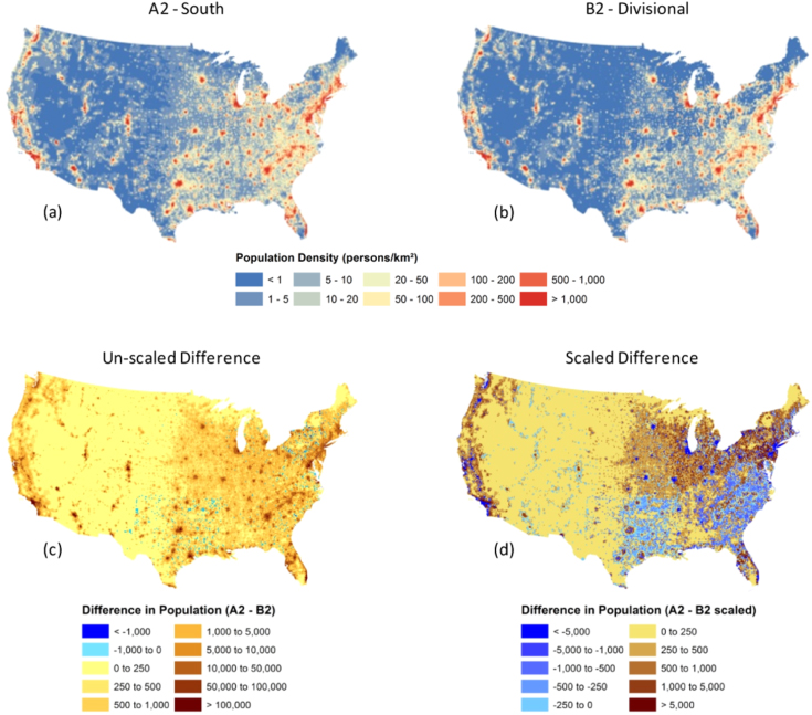
Figure 1. NCAR national (a) A2 and (b) B2 scenarios, (c) grid-cell specific difference in total population, and (d) grid-cell specific difference in total population when the A2-national population is scaled to match the total B2 population.
Download figure:
Standard image High-resolution image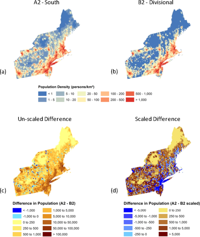
Figure 2. NCAR (a) A2 and (b) B2 scenarios for the northeast census region, (c) grid-cell specific difference in total population, and (d) grid-cell specific difference in total population when the A2-national population is scaled to match total B2 population.
Download figure:
Standard image High-resolution imageDifferences in outcomes between the A2 and B2 scenarios (figures 1 and 2) are due in part to differences in projected aggregate urban and rural population change at the division-level. Both the projected total and urban populations in 2100 are larger in the A2 scenario, by 26% and 33% respectively. Conversely, the rural population is projected to decline at a faster rate in the A2 scenario, leading to a rural population 28% smaller than in the B2 scenario. As a result, in general the A2 scenario projects higher population densities, particularly in urban and suburban areas. Cities in the West and South exhibit particularly large differences (figure 1(c)). However, the fact that the A2 scenario assumes a more sprawling pattern of spatial development also plays a role, evident in higher population densities in areas surrounding the larger cities of the Northeast, Midwest, and West Coast.
Population density in rural areas appears to be counter to expectations based on the differences in aggregate rural populations: most of the area currently considered mainly rural has higher population densities in the A2 scenario despite that scenario's lower aggregate rural population projection (figure 1(c)). This outcome is driven by faster-growth of the aggregate urban population in the A2 scenario combined with parameters promoting a more sprawling pattern of development, which tends to push growing urban populations into rural areas. Only a few cells actually exhibit higher densities in rural areas under the B2 scenario, mostly in the Mid-Atlantic, South Atlantic, and West South Central divisions. In the Mid-Atlantic, this is due to a relatively low urban population growth rate in the A2 scenario, thus urban expansion is not enough to make up for rural population decline. In the South Atlantic and West South Central, it is due to especially high rural population losses in the A2 scenario.
In figures 1(d) and 2(d) the A2 population has been scaled to the B2-national total, thus the variation in spatial distribution is primarily a result of the different parameter estimates employed (a minor difference in the urbanization rate accounts for a small amount of the variation in these figures). Significant variation in urban/suburban-style growth exists between scenarios in the Northeast, Midwest, and West Coast. The sprawling pattern of development associated with the A2 storyline leads to growth that, relative to the B2 scenario, is far more horizontal. As a result proportionally more growth takes place in suburban areas outside of the major cities. Conversely, for most divisions the B2 projection has a more vertical pattern of development in which more growth, relative to the A2 scenario, is projected to occur within areas that are already highly urbanized. Figure 2(d) illustrates these differences in the Northeast census region; the pattern is particularly evident in the metro New York area.
The scenarios presented in figures 1 and 2 are just two of many possible spatial outcomes. We produced several variants of our A2 scenario to assess the sensitivity of population outcomes to different elements of the model (see the SI). Variant A2-Divisional assumes divisional population totals identical to those from our main scenario (A2-South), but employs parameter estimates for each of the nine census divisions in the A2 scenario (as opposed to South region estimates), yielding a projection in which the population of the Northeast, Midwest, and West Coast is more concentrated in urban areas (figure S8, available at stacks.iop.org/ERL/8/044021/mmedia). Variant A2-NoMigration (figure S9, available at stacks.iop.org/ERL/8/044021/mmedia) also uses division-specific parameter estimates but employs an alternative set of sub-national population projections that preserve the current (2000) proportional distribution of the national population, effectively assuming that the broad-scale redistribution of the population towards the south and west, a function of internal migration, will stop. The result is significantly higher densities in the northeast and midwest and lower densities in the west and south. Variant A2-National (figure S10, available at stacks.iop.org/ERL/8/044021/mmedia) applies the model at the national rather than divisional-level, distributing projected urban and rural change for the entire country across all grid-cells using a single set of parameters estimated from national-level change in the historical data. This scenario produces a broad distribution similar to that of the A2-NoMigration scenario, but the pattern of development in the northeast and midwest is more sprawling, while in the south and west it is more concentrated, differences that result from variation between national- and division-level parameter values.
4. Comparison to existing spatial projections
To further evaluate our results we compare our A2 scenario (figure 1) to 100-year spatial outcomes from the EPA and IIASA A2 scenarios (figures 3(a) and (b)). The NCAR and IIASA scenarios have identical population growth assumptions, including aggregate urban/rural totals. The EPA model projects a significantly larger total population (688 million in 2100 versus 470 million in the IIASA/NCAR projections) and does not differentiate between urban and rural persons. In comparison to our A2 scenario the EPA model projects larger populations in areas considered urban and/or suburban (figure 2(c)), and in general projects a vertical pattern of development in which populations grow relatively quickly and in a concentrated pattern in existing urban agglomerations. This difference is a result of the gravity framework used to estimate migration in the EPA county-level population projections, which is heavily influenced by the existing population structure such that internal migration is directed primarily towards counties with large populations, leading to slow-growth in smaller counties and rapid growth in already heavily populated counties. Furthermore, because urban counties often serve as 'gateways' for immigration into the United States, the bulk of the projected immigrant population is allocated into cities [21]. As an example, the EPA model projects larger populations across most of the metropolitan New York City area. There are some exceptions to this general tendency, however. In cities like Dallas and Houston the EPA model projects more growth on the urban fringe and in suburban areas while the NCAR model projects a larger population in the urban core. These results indicate that the land-use and infrastructure components of the EPA allocation mechanism may be steering population away from the already congested interior of certain cities, particularly those in which nearby land is less-developed and good transportation infrastructure is in place. This mechanism only operates within counties however, since across-county allocation is controlled exogenously, and so is more evident in areas like the south and west where county sizes are large.
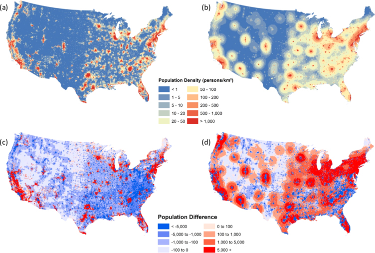
Figure 3. National A2 scenarios from the (a) EPA and (b) IIASA, and (c) and (d) grid-cell specific population difference with the NCAR A2 scenario (NCAR projection scaled to match the total population in the EPA projection in figure 2(c)). Blues indicate higher values in the NCAR projection.
Download figure:
Standard image High-resolution imageThe IIASA A2 scenario, in stark contrast to the EPA scenario, is characterized by considerable urban expansion, the development of large urban corridors, and a population that is significantly more dispersed than in the NCAR projection (figure 3(b)). The pattern of urban expansion projected throughout the IIASA scenario results from using an inverse distance-squared function to weight distance in the calculation of potential. Relative to observed patterns of population change this commonly used formulation of potential produces a very shallow population change gradient leading to excessive urban expansion. The propensity of the model towards sprawl is compounded by the self-potential problem [35, 36], which by excluding any contribution from the population of each cell to its own potential further enhances the model's tendency towards smoothing the distribution.
The IIASA methodology also projects a more uniform pattern of change across the US relative to the EPA and NCAR scenarios, due in part to the lack of a geospatial mask limiting future allocation. For example, consider the metro Denver area situated on the Front Range of the Rocky Mountains. The IIASA scenario projects a constant pattern of spatial change in a circular pattern around Denver, while the EPA and NCAR models project development in a narrow north–south corridor mirroring the mountains. The lack of some measure of slope and elevation leaves only straight-line proximity to govern future allocation, leading to the symmetric pattern in the IIASA projections. Similar population growth is projected (in the IIASA scenario) into the Florida Everglades to the west of Miami due to the lack of accounting for protected land and areas in which surface water is present.
Another notable difference between the IIASA and NCAR projections is evident in the northeast and midwest regions, where the IIASA model projects higher populations throughout almost the entire area. The opposite is true in the south region (albeit not to the same degree) where the NCAR model projects higher populations across much of the area. These differences result from variation in the spatial level of aggregation at which each model was applied. The IIASA scenario allocates projected change in the national urban and rural populations across all grid-cells (similar to our A2-National variant), while the NCAR scenario allocates projected change in aggregate divisional population across each of the nine census divisions, a measure that includes the impact of inter-divisional migration. As such, the NCAR results reflect a projected continuation of the ongoing broad-scale population redistribution away from the northeast and midwest and towards the south and west, leading to smaller populations in the former and larger in the latter relative to the IIASA results.
5. Metrics
From scenario-based gridded distributions we can derive a variety of potentially useful metrics describing aspects of the distribution that may be important in particular applications, such as impacts, adaptation, and vulnerability (IAV) research. For example, assessment of the potential future vulnerability to climate-related hazards such as coastal storms and/or sea-level rise requires a measure indicating the proximity of future populations to the coastline. Figure 4 illustrates this metric for the NCAR A2 and B2 scenarios, as well as the IIASA and EPA A2 scenarios at 10 km intervals for the state of Florida. Immediately it is apparent that between-model variation is much larger than the between-scenario variation in the NCAR A2/B2 results. Projected population totals within 20 km of the coast range from nearly no change relative to the base-year (IIASA) to over 250% growth (EPA). Both NCAR scenarios fall between these more extreme results.
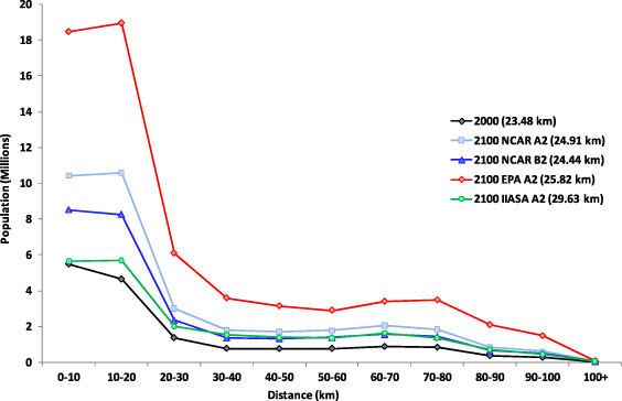
Figure 4. Projected population of Florida in 2100 by distance to the coast for the NCAR, EPA, and IIASA A2 scenarios, and the NCAR B2 scenario. Observed population in 2000 is shown for comparison, and the average distance to the coast is noted in parentheses in the legend.
Download figure:
Standard image High-resolution imageThis variation results from differences in projected population at three different scales. First, national-level population change is largest in the EPA scenario, which projects 146% growth by the end of the century compared to 68% growth in the IIASA and NCAR scenarios. Second, the proportion of the population residing in Florida is largest in the EPA scenario, because EPA county-level population projections assume continued high-levels of in-migration to urban counties in Florida, and thus significant population growth. Third, within Florida, the portion of the population allocated to coastal areas is largest in the NCAR B2 scenario, due primarily to parameter estimates that are less indicative of expansion and thus proportionally more development closer to the coastline relative to the A2 scenarios.
All four scenarios project a population that, on average, moves slightly inland over time. In 2000 the average Floridian lived roughly 23.5 km from the coastline. Average distance for NCAR B2 scenario, which produces less inland expansion then any of the A2 scenarios, is approximately 1 km greater. Among the A2 scenarios the NCAR model projects the most 'coastal' population, with an average distance of roughly 25 km. The EPA model, driven by county-level population projections, predicts an average distance of just under 26 km, while the IIASA model, which projects rapid inland expansion, produces a much higher average distance of nearly 30 km.
The degree to which a population is dispersed or consolidated, or alternatively tends towards horizontal or vertical development, will affect infrastructure, energy consumption, and impacts on habitat. Figure 5 shows two different measures of this dispersion: the amount of land, or of population, by population density. A more dispersed settlement pattern would be indicated by a larger proportion of people living in low-density areas, and a more even distribution of land by density class. In addition to the NCAR A2 scenario, which uses parameter estimates from the south region, we show an A2-northeast variant using parameter estimates from the northeast to investigate the implications of the continuation of the region's own historical patterns of development.

Figure 5. Number of grid-cells (solid lines) and total population (dashed lines) in 2100 in the A2 scenario by population density class, aggregated over the northeast census region. Results are shown for the EPA (red) and IIASA (green) models, as well as for the NCAR model with parameter estimates from the northeast region (dark blue) and south region (light blue).
Download figure:
Standard image High-resolution image
Again it is evident that substantial between-model variation exists. The overall levels of population vary due to differences in projected population for the region as a whole—a result of differences both in national-level population and in broad-scale regional distributions—but the patterns of population and land by density class are due to differences in spatial allocation. The EPA projection is consistent with a very concentrated pattern of development, where the bulk of the land area remains lightly populated (as indicated by the large number of cells in the low-density classes) and the majority of the population is found in high-density areas. By contrast the IIASA model tends towards a sprawling settlement pattern in which the bulk of the land area can be classified as medium-density and a large proportion of the population resides in medium-density cells, with fewer people in high-density cells than the EPA model. The NCAR scenarios are indicative of a more moderate spatial development pattern, less concentrated than the EPA projection, but without the extreme sprawl found in the IIASA scenario.
The NCAR scenario is sensitive to the parameter values employed. The northeast and south parameter variants are similar in terms of the distribution of population across density classes (although there are about 3 million more people in the highest-density cells in the northeast scenario), but the distribution of grid-cells (or land) by density class is significantly different. The northeast variant projects far more lightly populated land and somewhat more of the most densely settled land, while the A2-south scenario projects much more land in the medium-density range. These differences reflect the more concentrated development experienced historically in this region, as captured in the northeast parameter values, compared to the more sprawling development induced by the south region parameters. The population-weighted average grid-cell density in the northeast scenario is much higher (1905 km−2) than in the south scenario (1609 km−2), reflecting a future in which the average person in the northeast region lives in a higher-density settlement.
Additional metrics could be devised to summarize aspects of the population distribution relevant to other uses, for example assessing the relationship between population and watersheds, ecosystem types, or threatened habitats. The results shown here illustrate the potential for a wide range of possible outcomes across scenarios, models, and parameter values, emphasizing the need for improved understanding of determinants of spatial outcomes and better measures of their characteristics.
6. Discussion
In this work we develop and apply a new model for downscaling aggregate urban and rural population projections to produce spatially explicit future population scenarios. Our work is motivated by the increasing demand for spatial population projections in the global change research community, and is informed by existing large-scale models. Key features of the model include its flexibility in producing alternative outcomes that are consistent with qualitative global change narratives and the ability to calibrate the model to historical data. We can consider alternative national and sub-national projections of urban and rural change, apply the model at different levels of spatial aggregation, employ alternative parameter values that correspond to desired patterns of development or are estimated from historical data, and vary assumptions regarding habitable land. The gravity framework is advantageous in that it is easily expanded or altered to consider additional parameters and/or alternative mathematical forms of distance decay [36]. Similarly, within the framework of the existing model, it may be possible to correlate patterns of spatial change as characterized by the α and β parameters to certain demographic/socio-economic indicators, facilitating both additional exploration into the possible drivers of spatial change and projections guided explicitly by these indicators. The spatial mask could be expanded to include additional geophysical characteristics deemed important, including those that are not temporally static such as projected changes in coastlines, and the gravity field can easily accommodate additional detail including, but not limited to, the projected availability of certain resources, anticipated response to climate feedbacks, and policy designed to influence settlement patterns. Projecting resource availability, policy, and other important indicators into the future was beyond the scope of this work, which was designed specifically to explore a new modeling framework and to improve upon existing large-scale spatial projections. However, as a tool for generating scenarios and exploratory research the gravity structure appears to hold significant promise.
Results from our application of the model to spatial projections consistent with the SRES A2 and B2 scenarios show that alternative parameter values do indeed drive local variation in patterns of spatial change, particularly in urban/suburban areas. For example, urban expansion in the A2 scenario occurs in a more horizontal fashion, a result of applying parameter estimates calibrated to a region of the US that has experienced sprawling development patterns. We also find that our results show substantial differences from two existing projections for the US from IIASA and the EPA based on the same SRES scenarios. Between-model variation (IIASA, EPA, and NCAR A2) is significantly larger than between-scenario (NCAR A2/B2) variation for two metrics important for possible implications for environmental consequences: population distribution by distance from the coast, and either population or land distribution by population density. A key factor driving differences across models is the spatial scale at which downscaling occurs: the IIASA and EPA scenarios represent opposite extremes in the level of aggregation of exogenous projections, national- and county-level respectively, while our scenario was constructed using an intermediate aggregation, the US census division. These differences affect the degree to which different models can capture broad-scale changes of sub-national population distribution. In addition, the local behavior of the models differs. Thus, assumptions concerning both broad- and local-scale patterns of spatial change inherent in the structure of a given model are significant factors in spatial population outcomes, and may influence results moreso than variation in assumptions regarding national-level population change or urbanization.
These findings suggest that substantial further work on spatial population modeling is warranted in order to provide plausible, well grounded projections for use in global change research. In particular, understanding the influence of model structure, the importance of calibration to historical data, additional means of validation across a variety of scales, and the influence of broad-scale redistribution patterns should be a high priority. The model presented here is designed to produce plausible alternative spatial scenarios grounded by historical patterns of change and/or corresponding to specific qualitative narratives in a consistent manner, enabling between-scenario examination. Large-scale spatially explicit models of spatial population change remain relatively young, and would continue to benefit from additional work regarding the factors driving spatial change at multiple scales.